Note on the Coulomb blockade of a weak tunnel junction with Nyquist noise: Conductance formula for a broad temperature range

Abstract

We revisit the Coulomb blockade of the tunnel junction with conductance much smaller than $e^{2}/\hbar$. We study the junction with capacitance $C$, embedded in an Ohmic electromagnetic environment modelled by a series resistance $R$ which produces the Nyquist noise. In the semiclassical limit the Nyquist noise charges the junction by a random charge with a Gaussian distribution. Assuming the Gaussian distribution, we derive analytically the temperature-dependent junction conductance $G(T)$ valid for temperatures $k_{B}T\gtrsim(R_{K}/2\pi R)E_{c}$ and resistances $R\gtrsim R_{K}$, where $R_{K}=h/e^{2}$ and $E_{c}=e^{2}/2C\ \text{is}$ the single-electron charging energy. Our analytical result shows the leading dependence $G(T)\propto e^{-E_{c}/4k_{B}T}$, so far believed to exist only if $(R_{K}/\pi R)E_{c}\ll k_{B}T\ll E_{c}$ and $R\gg R_{K}$. The validity of our result for $k_{B}T\gtrsim(R_{K}/2\pi R)E_{c}$ and $R\gtrsim R_{K}$ is confirmed by a good agreement with the numerical studies which do not assume the semiclassical limit, and by a reasonable agreement with experimental data for $R$ as low as $R_{K}$. Our result also reproduces various asymptotic formulae derived in the past. The factor of $1/4$ in the activation energy $E_{c}/4$ is due to the semiclassical Nyquist noise.

I I. Introduction

Electron tunneling in a small tunnel junction is affected by the electromagnetic environment which gives rise to the Coulomb blockade. Since the resulting current-voltage characteristics depends on the type of the environment, one speaks about a coupled junction-environment system Averin ; Delsing ; NazarovJPT ; SchoenZaikin ; IngoldNazarov . Starting from these ideas, the Coulomb-blockaded current-voltage characteristics of the coupled junction-environment system was derived for a so-called weak tunnel junction DevoretPRL ; GirvinPRL which has the tunnel conductance much smaller than $e^{2}/h$. Later, the theory was extended for a junction with arbitrary strong tunneling JoyezPRL . The theory DevoretPRL ; GirvinPRL ; JoyezPRL gives a formal result for the current voltage characteristics, however, analytical results are known Averin ; AverinBook ; DevoretPRL ; GirvinPRL ; GerdSchoen ; GrabertNATOARW ; Ingold94 ; IngoldHabilitation ; Heikilla ; Panyukov ; Kauppinen ; Wang ; JoyezPRB only for a special limits and a full comparison of the theory and experiment JoyezPRL requires a numerical calculation JoyezPRB ; Odintsov . In particular, a temperature-dependent junction conductance, $G(T)$, was derived analytically Averin ; AverinBook ; Panyukov ; Kauppinen ; Wang ; JoyezPRB either for $k_{B}T\gg E_{c}$ or for $k_{B}T\ll E_{c}$, where $E_{c}=e^{2}/2C$ is the single-electron charging energy of the junction with capacitance $C$. As far as we know, for the temperature range from $k_{B}T\gg E_{c}$ down to $k_{B}T\ll E_{c}$ only the numerical studies of $G(T)$ are known GirvinPRL ; JoyezPRL ; JoyezPRB ; Flensberg .

Here we revisit the Coulomb blockade of the weak tunnel junction with the aim to derive analytically $G(T)$ for a broad temperature range. We consider the junction with capacitance $C$, embedded in an electromagnetic environment modeled by a series resistance $R$ which produces the Nyquist noise. In the semiclassical limit the Nyquist noise charges the junction by a random charge with a Gaussian distribution IngoldNazarov ; GerdSchoen ; Heikilla . Assuming the Gaussian distribution, we derive an analytical $G(T)$ expression valid for $k_{B}T\gtrsim(R_{K}/2\pi R)E_{c}$, where $R_{K}=h/e^{2}$ and $R\gtrsim R_{K}$.

Our $G(T)$ expression shows the leading dependence $G(T)\propto e^{-E_{c}/4k_{B}T}$, so far known Averin ; Odintsov to exist only in conditions $(R_{K}/\pi R)E_{c}\ll k_{B}T\ll E_{c}$ and $R\gg R_{K}$. The validity of our result for $k_{B}T\gtrsim(R_{K}/2\pi R)E_{c}$ and $R\gtrsim R_{K}$ is confirmed by a good agreement with the numerical studies GirvinPRL ; JoyezPRL ; JoyezPRB ; Flensberg which do no rely on the semiclassical limit, and by a reasonable agreement with experimental data JoyezPRL for $R\simeq R_{K}$. Our result also reproduces various asymptotic formulae derived in the past Averin ; Wang ; JoyezPRB . Finally, we point out that the factor of $1/4$ in the activation energy $E_{c}/4$ is due to the Nyquist noise and we add a simple treatment of the noise in the semiclassical limit.

Sect. II starts with a review of the weak tunnel junction theory DevoretPRL ; GirvinPRL which serves as our starting point. Then we derive $G(T)$. In Sect.III our results are discussed and compared with previous works. A summary is given in Sect. IV and we finish with an appendix which discusses the Nyquist noise within a semiclassical transport model. This paper is a refined version of our recent arXiv attempts arXiv .

II II. Theoretical considerations

We first briefly review the weak tunnel junction theory DevoretPRL ; GirvinPRL . Figure 1a shows two electron gases separated by energy barrier $V_{0}$. Assume that the electrons pass through the barrier only by tunneling. The junction conductance without the Coulomb blockade, $G_{t}$, obtained from a golden-rule approach, reads $G_{t}=(4\pi e^{2}/\hbar)N_{l}N_{r}\mid\mathcal{T}\mid^{2}$, where $\mathcal{T}=<r\mid H_{t}\mid l>$ is the matrix element (approximated by a constant) for tunneling from an initial state $\mid l>$ on the left hand side of the barrier to a final state $\mid r>$ on the right hand side, $N_{l/r}$ is the density of states at the Fermi energy on the left/right hand side, and $H_{t}$ is the weakly-perturbing tunneling Hamiltonian FerryGoodnick ; Pfannkuche .

In the electric circuit of figure 1b the junction with capacitance $C$ and tunneling conductance $G_{t}$ is coupled to a constant voltage source $V_{x}$ via the impedance $Z(\omega)$ which represents the impedance of the external circuit. This impedance, defined as $Z(\omega)=U(\omega)/I(\omega)$, gives the ratio between an alternating voltage of frequency $\omega$ and the current which is flowing through it if the junction is replaced by a short IngoldNazarov ; DevoretPRL ; GerdSchoen ; Heikilla . Due to the coupling to the external circuit the voltage drop at the junction fluctuates but its average value $V$ fulfills the Kirchhoff law GerdSchoen

$$V+I(V)Z(0)=V_{x}\ ,$$ (1)

where $I(V)$ is the current-voltage characteristic. The junction can be reduced to a capacitor if $1/G_{t}\gg Z(\omega)$ GerdSchoen ; Heikilla . In such case the total impedance at the site of the junction is GerdSchoen ; Heikilla $Z_{t}(\omega)=1/[i\omega C+1/Z(\omega)]$.

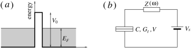
Figure 1: (a) Conduction band edge in a tunnel junction due to two weakly linked metals. (b) Tunnel junction in the circuit.

Further, $I(V)=e[\Gamma^{+}(V)-\Gamma^{-}(V)]$, where GerdSchoen ; IngoldHabilitation

$$\Gamma^{+}(V)=\frac{G_{t}}{e^{2}}\int_{-\infty}^{\infty}dE\frac{E}{1-\exp{(-E/k_{B}T)}}P(eV-E)\$$ (2)

is the rate of tunneling from the left reservoir to the right one, $\Gamma^{-}(V)=\Gamma^{+}(-V)$ is the tunneling rate in the opposite direction, and function $P(E)$ is the probability that a tunneling electron creates an environmental excitation with energy $E$. The above equations give DevoretPRL ; GerdSchoen ; JoyezPRB

$$\begin{split}I(V)&=\frac{G_{t}}{e}\int_{-\infty}^{\infty}dE\frac{E}{1-\exp{(-E/k_{B}T)}}\\ &\times[P(eV-E)-P(-eV-E)]\ .\end{split}$$ (3)

Function $P(E)$ is related DevoretPRL ; GerdSchoen ; JoyezPRB to the correlation function $J(t)=<[\phi(t)-\phi(0)]\phi(0)>$ of the phase $\phi(t)=\int_{-\infty}^{t}dt[eU(t)-eV]$ across the impedance $Z_{t}$. Specifically,

$$P(E)=(1/2\pi\hbar)\int_{-\infty}^{\infty}dt\exp{[J(t)+iEt/\hbar]}\ .$$ (4)

Finally, from the fluctuation dissipation theorem one finds

$$J(t)=2\int_{-\infty}^{\infty}\frac{d\omega}{\omega}\frac{\mathrm{Re}{\{Z_{t}(\omega)\}}}{R_{K}}\frac{\exp{(-i\omega t)}-1}{1-\exp(-\frac{\hbar\omega}{k_{B}T})}\ ,$$ (5)

where $R_{K}\equiv h/e^{2}$ is the resistance quantum DevoretPRL ; GerdSchoen ; IngoldHabilitation ; JoyezPRB .

The above theory is assumed to hold if $H_{t}$ is a weak perturbation and $1/G_{t}\gg Z(\omega)$. Moreover, it has to be fulfilled that $1/G_{t}\gg R_{K}$, which ensures Korotkov that a single-electron tunnel event takes a much shorter time than the time between two events. The electrons are thus mostly localized on the electrodes, which is an implicit assumption of the model in figure 1b. We will see later that the condition $1/G_{t}\gg R_{K}$ can be soften to Heikilla $1/G_{t}\gg R_{K}/2\pi$ and condition $1/G_{t}\gg Z(\omega)$ is likely too stringent as well.

We consider the Ohmic environment GerdSchoen ; Heikilla $Z(\omega)=R$, for which $\mathrm{Re}{\{Z_{t}(\omega)\}}=R/(1+\omega^{2}R^{2}C^{2})$. For $R\gg R_{K}$ one has $\mathrm{Re}{\{Z_{t}(\omega)\}}=(\pi/C)\delta(\omega)$ and one obtains GerdSchoen ; Heikilla the result $J(t)=-\pi/(CR_{K})[it+k_{B}Tt^{2}/\hbar]$ valid GerdSchoen for $\hbar/RC\ll k_{B}T$. Setting the last $J(t)$ expression into the equation (4) one finds GerdSchoen ; Heikilla

$$P(E)=\frac{1}{\sqrt{4\pi k_{b}TE_{c}}}\exp{\left[-\frac{(E-E_{c})^{2}}{4k_{b}TE_{c}}\right]},\ k_{B}T\gg\frac{\hbar}{RC},$$ (6)

where $E_{c}\equiv e^{2}/2C$. This limit is called semiclassical and the Gaussian spread of the distribution (6) is due to the Nyquist noise produced by resistance $R$. To see all this in a simple way, in the appendix we derive the Nyquist noise and probability (6) from a semiclassical transport model.

Now we derive the conductance $G$ which relies on the approximation (6). Thus, our derivation should be valid only for $k_{B}T\gg\hbar/RC$ and $R\gg R_{K}$. However, we will see that the obtained conductance result works quite well down to $k_{B}T\simeq\hbar/2RC$ and $R\gtrsim R_{K}$.

We rewrite equation (3) for $V\rightarrow 0$ as

$$I(V)=G_{t}\int_{-\infty}^{\infty}dE\frac{2E}{1-\exp{(-E/k_{B}T)}}\frac{dP(-E)}{d(-E)}V\ .$$ (7)

Replacing $-E$ by $E$ and inserting for $P(E)$ the equation (6) we obtain the Ohm law $I=GV$, where

$$\begin{split}G&=\frac{G_{t}}{\sqrt{4\pi k_{b}TE_{c}}}\int_{-\infty}^{\infty}dE\frac{2E}{\exp{(E/k_{B}T)}-1}\\ &\times\ \frac{d}{dE}\left(\exp{\left[-\frac{(E-E_{c})^{2}}{4k_{b}TE_{c}}\right]}\right)\ ,\ \ \ \ \ k_{B}T\gg\frac{\hbar}{RC}\ .\end{split}$$ (8)

The integral in equation (8) cannot be calculated analytically. However, we can use a simple trick which allows us to asses $G(T)$ for all considered $T$ without such calculation. Using $x=E/2k_{B}T$ and $\alpha\equiv E_{C}/k_{B}T$ we get

$$\begin{split}\frac{G}{G_{t}}&=\frac{1}{\sqrt{\pi\alpha}}\int_{-\infty}^{\infty}dx\frac{2x}{\exp{(2x)}-1}\\ &\times\ \frac{d}{dx}\left(\exp{\left[-\left(\frac{x}{\sqrt{\alpha}}-\frac{\sqrt{\alpha}}{2}\right)^{2}\right]}\right)\ ,\end{split}$$ (9)

where $1/\alpha\gg R_{K}/\pi R$. After a simple calculation we get

$$\frac{G}{G_{t}}=\exp{\left(-\frac{\alpha}{4}\right)}I({\alpha})\ ,\ \ \ \ \ \ \ \ \frac{1}{\alpha}\gg\frac{R_{K}}{\pi R}\ ,$$ (10)

where

$$I(\alpha)=\frac{1}{\sqrt{\pi\alpha}}\int_{-\infty}^{\infty}dx\exp{\left(-\frac{x^{2}}{\alpha}\right)}\frac{x}{\sinh(x)}\ ,$$ (11)

or alternatively, by means of variable $y=x/\sqrt{\alpha}$,

$$I(\alpha)=\frac{1}{\sqrt{\pi}}\int_{-\infty}^{\infty}dy\exp{\left(-y^{2}\right)}\frac{\sqrt{\alpha}y}{\sinh(\sqrt{\alpha}y)}\ .$$ (12)

Equation (10) is a useful alternative form of equation (8).

From equation (10) we obtain the leading dependence

$$\frac{G}{G_{t}}\simeq\exp{\left(-\frac{\alpha}{4}\right)}=\exp{\left(-\frac{E_{c}}{4k_{B}T}\right)}\ ,\ \ \ \ \frac{1}{\alpha}\gg\frac{R_{K}}{\pi R}\ .\ \$$ (13)

Indeed, for $\alpha\rightarrow 0$ we find from equation (11) result $I(0)=1$ while for $\alpha\gg 1$ we find

$$I(\alpha)\simeq\frac{1}{\sqrt{\pi\alpha}}\int_{-\infty}^{\infty}dx\ \frac{x}{\sinh{x}}=\sqrt{\frac{\pi^{3}}{4\alpha}}\ ,$$ (14)

because $\exp{(-x^{2}/\alpha)}\rightarrow 1$ for $\mid x\mid\lesssim\sqrt{\alpha}$ and $x/\sinh{(x)}$ is peaked at $x=0$. We see that $I(\alpha)$ decays with increasing $\alpha$ from $I(0)=1$ towards the weak dependence $I(\alpha)=\sqrt{\pi^{3}/4\alpha}$ at large $\alpha$. Thus, the leading dependence in equation (10) is indeed $\exp{(-\alpha/4)}$ for any $\alpha$.

To get beyond the leading dependence (13) we examine again the factor $I(\alpha)$. For $\alpha\ll 1$ we can use expansion

$$\frac{\sqrt{\alpha}y}{\sinh(\sqrt{\alpha}y)}=1-\frac{\alpha}{6}y^{2}+\frac{7\alpha^{2}}{360}y^{4}+O[(\sqrt{\alpha}y)^{6}]\ .$$ (15)

Inserting expansion (15) into the equation (12) we obtain

$$I(\alpha)=1-\frac{\alpha}{12}+\frac{7\alpha^{2}}{480}+O\left[\alpha^{3}\right]\ ,\ \ \ \ \ \ \alpha\ll 1\ .$$ (16)

For $\alpha\gg 1$ we can use expansion

$$\exp{\left(-\frac{x^{2}}{\alpha}\right)}=1-\frac{x^{2}}{\alpha}+\frac{x^{4}}{2\alpha^{2}}+O\left[(x/\sqrt{\alpha})^{6}\right]\ .$$ (17)

Setting expansion (17) into the equation (11) we obtain

$$I(\alpha)=\sqrt{\frac{\pi^{3}}{4\alpha}}\left[1-\frac{1}{\alpha}\frac{\pi^{2}}{2}+\frac{1}{\alpha^{2}}\frac{\pi^{4}}{2}+O\left(\frac{1}{\alpha^{3}}\right)\right]\ ,$$ (18)

where $\alpha\gg 1$. For large enough $\alpha$ the last equation reduces to $I(\alpha)\simeq\sqrt{\pi^{3}/4\alpha}$, in accord with limit (14). Finally, we propose a simple but very precise interpolation between $I(0)=1$ and $I(\alpha\gg 1)=\sqrt{\pi^{3}/4\alpha}$, namely

$$I(\alpha)\simeq\left(1+4\alpha/\pi^{3}\right)^{-1/2}\ .$$ (19)

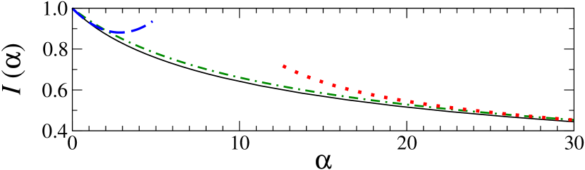
Figure 2: Factor $I(\alpha)$ versus $\alpha$. The full line is obtained by calculating numerically the integral (11). Interpolation (19) is shown in a dotted-dashed line. Limits (16) and $\eqref{correction big22}$ are shown in a dashed line and in a dotted line, respectively.

One can see in figure 2 that the interpolation (19) fits the exact $I(\alpha)$ almost perfectly while expansions (16) and $\eqref{correction big22}$ work only for a too small or too large $\alpha$. Combining equations (19) and (10) we obtain the result

$$\frac{G}{G_{t}}\simeq\left(1+\frac{4\alpha}{\pi^{3}}\right)^{-1/2}\exp{\left(-\frac{\alpha}{4}\right)}\ ,\ \ \ \ \ \ \frac{1}{\alpha}\gg\frac{R_{K}}{\pi R}\ ,$$ (20)

which goes beyond the leading approximation (13). Since the interpolation (19) works very well, result (20) agrees with the exact result (10) almost perfectly.

Results (10), (13), and (20) did not yet appear in the literature. In the next section we will see that the restriction $1/\alpha\gg R_{K}/\pi R$ can be soften to $1/\alpha\gtrsim R_{K}/2\pi R$.

Noteworthy, $G/G_{t}\simeq\exp{(-E_{c}/4k_{B}T)}$ is the Arhenius dependence with activation energy $E_{c}/4$ rather than $E_{c}$. We wish to point out that the factor of $1/4$ in the activation energy $E_{c}/4$ is due to the Nyquist noise. First of all, as shown in the appendix, the Nyquist noise gives rise to the finite width of the distribution (6). If we ignore the noise and replace the distribution (6) by $P(E)=\delta(E-E_{c})$, the equation (8) reduces to

$$\frac{G}{G_{t}}=\int_{-\infty}^{\infty}dE\frac{2E}{\exp{(E/k_{B}T)}-1}\ \frac{d}{dE}\delta(E-E_{C})\\ .$$

From the last equation one readily obtains (for $k_{B}T\ll E_{c}$) the leading dependence $G\propto\exp{(-E_{c}/k_{B}T)}$. Unlike the dependence $G\propto\exp{(-E_{c}/4k_{B}T)}$, this leading dependence does not contain the factor of $1/4$.

The leading dependence $G\propto\exp{(-E_{c}/4k_{B}T)}$ has been derived already in Refs. Averin and Odintsov , however, only for $(R_{K}/\pi R)E_{c}\ll k_{B}T\ll E_{c}$. We have just shown that it is valid for $k_{B}T\gg(R_{K}/\pi R)E_{c}$ and we will extend this range of validity even more in the next section.

III III. Discussion of results, comparison with previous works, asymptotic behavior

We have derived the formulae (10), (13), and (20) by considering the conditions $G_{t}^{-1}\gg R\gg R_{K}$ and $k_{B}T\gg(R_{K}/\pi R)E_{c}$. The last condition implies that the formulae are applicable in a broad temperature range (from $k_{B}T\gg E_{c}$ down to $k_{B}T\ll E_{c}$) only if $R$ exceeds $R_{K}$ almost two orders of magnitude. Since a practically feasible values of $R$ are $R\sim R_{K}$ JoyezPRL ; Cleland , it may seem that the formulae (10), (13), and (20) are not applicable in practice. Surprisingly, we find below that they in fact work for temperatures $k_{B}T\gtrsim(R_{K}/2\pi R)E_{c}$ and resistances $R\gtrsim R_{K}$. This extends their applicability quite remarkably.

In figure 3 the formulae (10), (13), and (20) are compared with the numerical data JoyezPRB which hold for any $R$. More precisely, the calculation JoyezPRB is still restricted to a tunnel junction with $G_{t}^{-1}\gg R_{K}$ and $G_{t}^{-1}\gg R$, however, it is not restricted by assumptions $\pi R/R_{K}\gg E_{C}/k_{B}T$ and $R\gg R_{K}$ as it does not use the approximation (6).

As expected, results (20) and (10) almost coincide. Further, one can see that they agree with the numerical data JoyezPRB for $R/R_{K}=10$ in the whole temperature range. This is a surprising finding because for $R=10R_{K}$ the assumption $(R_{K}/\pi R)E_{c}\ll k_{B}T$ implies that the results (20) and (10) should deviate from the numerical data remarkably if $k_{B}T\lesssim E_{c}/\pi$. However, there is no deviation at all.

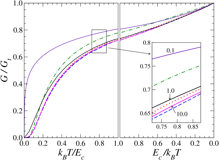
Figure 3: Conductance $G/G_{t}$ versus temperature. The full lines are the numerical data from Ref. JoyezPRB , obtained for $R/R_{K}=0.1$, $1$, and $10$. The dashed line shows our result (10) with $I(\alpha)$ calculated numerically and the dotted line shows our analytical approximation (20). The leading dependence $G/G_{t}=\exp{(-E_{c}/4k_{B}T)}$ is shown in a dotted-dashed line.

Moreover, we see that results (20) and (10) agree quite well also with the numerical data JoyezPRB for $R/R_{K}=1$. This is very surprising because $R=R_{K}$ contradicts the assumption $R\gg R_{K}$. Moreover, if we set $R=R_{K}$ into the assumption $(R_{K}/\pi R)E_{c}\ll k_{B}T$, we find that a good agreement can be expected only for $k_{B}T\gg E_{c}/\pi$. However, one can see a good quantitative agreement down to temperature as low as $k_{B}T\simeq 0.15E_{c}\simeq(R_{K}/2\pi R)E_{c}$ where the difference is about thirty percent (an acceptable error with regards to the decay by a factor of $\sim 6.5$). Moreover, one sees a qualitative accord for all temperatures.

We conclude that the restrictions $(R_{K}/\pi R)E_{c}\ll k_{B}T$ and $R\gg R_{K}$ can be soften to $(R_{K}/2\pi R)E_{c}\lesssim k_{B}T$ and $R\gtrsim R_{K}$, respectively. This extends the validity of the formulae (20) and (10) to a rather broad range of temperatures and series resistances, including the values $R\simeq R_{K}$ encountered in practice JoyezPRL .

Why the formulae work so well? It seems that the conductance is rather robust against the approximation (6). In this paper the robustness follows from comparison with the numerical data JoyezPRB not restricted by approximation (6) and we do not attempt to give an analytical explanation. Note in figure 3 that even the leading dependence $G/G_{t}=\exp{(-E_{c}/4k_{B}T)}$ alone is able to capture the main trend both for $R/R_{K}=1$ and $R/R_{K}=10$.

Finally, we see in figure 3 that the formulae (10), (13), and (20) fail to fit the numerical data JoyezPRB for $R/R_{K}=0.1$. In this case $R$ is simply too low and even the soft restriction $k_{B}T\gtrsim(R_{K}/\pi R)E_{c}$ is fulfilled only for very high $T$.

In figure 4, formulae (13) and (20) are compared with experimental data JoyezPRL for two samples and with theory JoyezPRL which holds for arbitrary $G_{t}$ and arbitrary $R$. It was reported JoyezPRL that $G^{-1}_{t}/R_{K}\simeq 1/3.07$ for sample ($1$) and $G^{-1}_{t}/R_{K}\simeq 1/22.8$ for sample ($2$). Moreover JoyezPRL , both samples posses the series resistance $R\simeq R_{K}$. Clearly, formulae (13) and (20) fail to fit the data for sample ($2$) because the sample is too far from regime $G_{t}^{-1}\gg R\gg R_{K}$. Sample ($1$) is more suitable in this respect and we expect a better fit. Indeed, both formulae mimic the S-shaped character of the data for sample ($1$) and even fit the data as $T$ increases towards $E_{c}/k_{B}$ and above. This is a reasonable experimental support that $G\propto\exp{(-E_{c}/4k_{B}T)}$ is the leading dependence in a broad temperature range. The discrepancy seen at low temperatures deserves a remark.

One source of the discrepancy is that also the sample ($1$) does not obey the condition $G_{t}^{-1}\gg R_{K}$ and hardly obeys even the softer version Heikilla $G_{t}^{-1}\gg R_{K}/2\pi$. However, overall trend of the presented data suggests that the discrepancy would become much smaller if the experimental value of $G_{t}^{-1}$ is enhanced only a few times. Thus, one can soften $G_{t}^{-1}\gg R_{K}$ to $G_{t}^{-1}\gtrsim R_{K}$, or to $G_{t}^{-1}\gg R_{K}/2\pi$ Heikilla . Another source of the discrepancy is that a sample with $R\simeq R_{K}$ does not fulfill well the condition $(R_{K}/2\pi R)E_{c}\lesssim k_{B}T$ as $T$ becomes low. It seems that the discrepancy would mostly disappear if one also enhances a few times the experimental value of $R$. Such sample would however still not fulfill the restriction $G_{t}^{-1}\gg R$ which suggests that this restriction is too stringent. This point needs a further investigation.

Inserting into the result $G/G_{t}=\exp{(-\alpha/4)}I(\alpha)$ the expansion $\exp{(-\alpha/4)}\simeq 1-\alpha/4+\alpha^{2}/32+O\left(\alpha^{3}\right)$ and expansion (16), we obtain the small $\alpha$ expansion

$$G/G_{t}\simeq 1-\alpha/3+\alpha^{2}/15+O\left(\alpha^{3}\right)\ ,$$ (21)

derived in Ref. JoyezPRB by a different method (equation (9) in Ref. JoyezPRB , taken for $R\gg R_{K}$). Similarly, the path-integral study Wang valid for junctions with arbitrary $G_{t}$ and $R$ reported a result which reproduces result (21) for $G^{-1}_{t}\gg R\gg R_{K}$. Unlike Refs. JoyezPRB ; Wang , our derivation of result (21) relies on the knowledge of the leading dependence $G/G_{t}\simeq\exp{(-\alpha/4)}$.

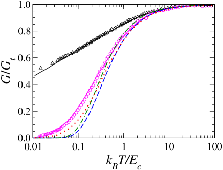
Figure 4: Conductance $G/G_{t}$ versus temperature. Our formulae (13) and (20) are shown in a dotted-dashed line and in a dashed line. The circles and triangles are the experimental data JoyezPRL for samples ($1$) and ($2$) which posses different values of $G_{t}$ and $R$ (see the text). The full lines are the numerical results JoyezPRL of the theory valid for an arbitrary $G_{t}$ and $R$. The numerical data JoyezPRL of the theory DevoretPRL ; JoyezPRB valid for small $G_{t}$ and arbitrary $R$ are shown in a dotted line. These data are the same for both samples.

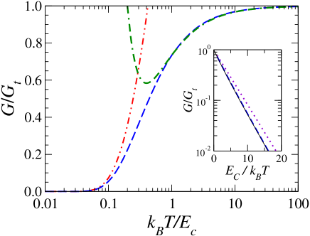
Figure 5: Conductance $G/G_{t}$ versus temperature. Formulae (20), (21), and (22) are plotted in a dashed line, in a dashed-double-dotted line, and in a dotted-double-dashed line, respectively. Inset: Arhenius plot $G/G_{t}$ versus $E_{c}/k_{B}T$. The dashed line and dotted line show the formulae (20) and (13), respectively. The full line shows the numerical data GirvinPRL obtained by solving equations (5), (4), (3), and (1) for $R\rightarrow\infty$. These data were taken from the inset in figure 3 of Ref. GirvinPRL , they essentially coincide with the numerical data JoyezPRB for $R/R_{K}=10$, shown in Fig. 3.

If $\alpha\gg 1$, $I(\alpha)\simeq\sqrt{\pi^{3}/4\alpha}$ and equation (10) gives

$$\frac{G}{G_{t}}\simeq\sqrt{\frac{\pi^{3}}{4\alpha}}\exp{\left(-\frac{\alpha}{4}\right)}\ ,\ \ \ \ \ \ \ \ \frac{R_{K}}{\pi R}\ll\frac{1}{\alpha}\ll 1\ ,$$ (22)

which coincides with the known result Averin ; AverinBook for $\alpha^{-1}\ll 1$, derived by a different approach. Also the equation (22) predicts the leading dependence $G/G_{t}\simeq\exp{(-\alpha/4)}$, however, only for small $\alpha^{-1}$ (for $k_{B}T\ll E_{c}$). The fact that the leading dependence $G/G_{t}\simeq\exp{(-\alpha/4)}$ holds (with restriction $1/\alpha\gg R_{K}/\pi R$) for any $\alpha$, can be concluded only from the exact result (10). Moreover, as we have shown, restriction $R_{K}/\pi R\ll 1/\alpha$ should be soften to $R_{K}/2\pi R\lesssim 1/\alpha$. Equation (22) with restriction $R_{K}/\pi R\ll 1/\alpha\ll 1$ is also given in Ref. Odintsov , but the leading dependence has a different pre-factor.

It may seem that results (10), (13), and (20) do not differ very much from result (22). The difference is however essential.

In figure 5 the formulae (22) and (21) are plotted together with our result (20). Unlike the result (20), they cannot mimic the S-shaped experimental curve in the preceding figure because they do not follow the leading dependence $G\propto e^{-E_{c}/4k_{B}T}$ in an essential temperature range. Let us mention that it does not help very much if we improve the formula (22) so that we replace the factor $\sqrt{\pi^{3}/4\alpha}$ by a more precise expansion (18).

The fact that the leading dependence $G\propto e^{-E_{c}/4k_{B}T}$ exists in a broad temperature range has been hidden in previous numerical studies GirvinPRL ; JoyezPRL ; JoyezPRB ; Flensberg . Specifically, a strong, essentially exponential (Arhenius) temperature dependence was found numerically GirvinPRL ; Flensberg by solving equations (5), (4), (3), and (1) for $R\rightarrow\infty$. In inset to figure 5, the Arhenius plot $G/G_{t}$ versus $E_{c}/k_{B}T$ found numerically in Ref. GirvinPRL is compared with the formula (20) and dependence $G/G_{t}=e^{-E_{c}/4k_{B}T}$. Obviously, the (almost) linear slope of the numerically generated Arhenius plot deviates from the slope $-E_{c}/4$. To recognize that the numerical data follow the leading dependence $G\propto e^{-E_{c}/4k_{B}T}$, one has to know result (20) or result (10).

If one sets the probability (6) into the equation (3) and assumes $T\rightarrow 0$, one finds analytically the well know DevoretPRL ; GirvinPRL ; GerdSchoen $I(V)$ characteristics $I=\frac{G_{t}}{e}(eV-E_{C})\Theta(eV-E_{c})$, where $\Theta(x)$ is the Heaviside step function. This $I(V)$ result shows the Coulomb gap of size $E_{C}$ at zero temperature. Noteworthy, the zero-voltage conductance $G\propto e^{-E_{c}/4k_{B}T}$ [results (10), (13), and (20)] shows the effective gap $E_{C}/4$ at any temperature, in reasonable accord with numerical studies and experiment.

Finally, regime $k_{B}T\gtrsim\hbar/RC$ studied here should not be confused with the opposite regime $k_{B}T\ll\hbar/RC$. In the latter regime the quantum noise takes place instead of the semiclassical Nyquist noise and the junction conductance shows IngoldNazarov ; GerdSchoen ; Panyukov ; SafiSauler the power law behavior $G/G_{t}\sim[(\pi R/R_{K})(2k_{B}T/E_{c})]^{(2R/R_{K})}$.

IV IV. Summary and concluding remarks

We have revisited the Coulomb blockade of the weak tunnel junction. We have analyzed the junction with capacitance $C$, connected in series with resistance $R$ which produces the Nyquist noise. In the semiclassical limit $k_{B}T\gg(R_{K}/2\pi R)E_{c}$ and $R\gg R_{K}$, the Nyquist noise charges the junction by a random charge with a Gaussian distribution. Assuming the Gaussian distribution, we have derived analytically the temperature-dependent junction conductance $G(T)$ which works surprisingly well for temperatures $k_{B}T\gtrsim(R_{K}/2\pi R)E_{c}$ and resistances $R\gtrsim R_{K}$. Our result shows the leading dependence $G(T)\propto e^{-E_{c}/4k_{B}T}$, so far believed Averin ; Odintsov to exist only in the limits $(R_{K}/\pi R)E_{c}\ll k_{B}T\ll E_{c}$ and $R\gg R_{K}$. The validity of our result for $k_{B}T\gtrsim(R_{K}/2\pi R)E_{c}$ and $R\gtrsim R_{K}$ has been confirmed by a good agreement with numerical studies GirvinPRL ; JoyezPRL ; JoyezPRB ; Flensberg which do no rely on the semiclassical limit, and by a reasonable agreement with experimental data JoyezPRL for $R$ as low as $R_{K}$. Finally, our result reproduces the known Averin ; AverinBook ; Wang ; JoyezPRB asymptotic formulae valid in limits $T\ll e^{2}/2Ck_{B}$ and $T\gg e^{2}/2Ck_{B}$.

Our result can be useful in simulations of the nano-scale devices which involve a nano-scale tunnel junction. Such junction is present say in a nano-scale field effect transistor roadmap or in a nano-scale memristor Zhirnov ; Waser .

V acknowledgement

This work was supported by grant VEGA 2/0200/14 and by Structural Funds of the European Union via the Research Agency of the Ministry of Education, Science, Research and Sport of the Slovak republic, project ”CENTE II” ITMS code 26240120019.

VI Appendix: Nyquist noise and distribution (6) from semiclassical transport model

Consider a metallic resistor with rectangular cross-section $L_{y}\times L_{z}$ and with length $L_{x}$ directed along the $x$ axis. Assume that the resistor is in thermodynamic equilibrium. The instantaneous electron current $i$, flowing in thermodynamic equilibrium in the $x$ direction, can be expressed as

$$i=\sum_{\textit{{k}},s}\frac{ev_{x}}{L_{x}}n(\textit{{k}},s)\ ,$$ (23)

where k is the electron momentum, $s$ is the electron spin, $n(\textit{{k}},s)$ is the occupation number of state $(\textit{{k}},s)$, $v_{x}=\hbar k_{x}/m$ is the electron velocity, and $m$ is the effective mass. The value of $n(\textit{{k}},s)$ fluctuates Kittel around the mean value $\langle n(\textit{{k}},s)\rangle=1/(\exp{[(\epsilon(\textit{{k}})-\mu)/k_{B}T]}+1)$ with variance

$$\langle n^{2}\rangle-\langle n\rangle^{2}=k_{B}T\frac{d}{d\mu}\langle n\rangle\ ,$$ (24)

where $\epsilon(\textit{{k}})=\hbar^{2}k^{2}/2m$ is the electron energy at the orbital $(\textit{{k}},s)$, $\mu$ is the chemical potential, and $\langle\dots\rangle$ is the ensemble average over the grand-canonical ensemble. Therefore, the equilibrium current $i$ fluctuates around the mean value

$$\langle i\rangle=\sum_{\textit{{k}},s}\frac{ev_{x}}{L_{x}}\langle n(\textit{{k}},s)\rangle=0$$ (25)

with variance

$$\begin{split}\langle i^{2}\rangle-\langle i\rangle^{2}=\langle i^{2}\rangle=\frac{e^{2}}{L^{2}_{x}}\sum_{\textit{{k}},s}\sum_{\textit{{k}}^{\bf{,}},s^{,}}v_{x}v^{,}_{x}&\\ \ \times[\langle n(\textit{{k}},s)n(\textit{{k}}^{\bf{,}},s^{,})\rangle-\langle n(\textit{{k}},s)\rangle\langle n(\textit{{k}}^{\bf{,}},s^{,})\rangle]\ .\end{split}$$ (26)

Assuming that each orbital is an independent grand-canonical system, we can use the equation

$$\begin{split}\langle n(\textit{{k}},s)n(\textit{{k}}^{\bf{,}},s^{,})\rangle-\langle n(\textit{{k}},s)\rangle\langle n(\textit{{k}}^{\bf{,}},s^{,})\rangle&\\ \ =[\langle n^{2}(\textit{{k}},s)\rangle-\langle n(\textit{{k}},s)\rangle^{2}]\delta_{\textit{{k}},\textit{{k}}^{\bf{,}}}\delta_{s,s^{,}}.\end{split}$$ (27)

If the last equation is combined with equation (24) and then inserted into the equation (26), we find

$$\langle i^{2}\rangle=k_{B}T\frac{e^{2}}{L^{2}_{x}}\sum_{\textit{{k}},s}v^{2}_{x}\frac{d}{d\mu}\langle n\rangle\ .$$ (28)

Using $\sum_{\textit{{k}},s}\rightarrow 2\frac{L_{x}L_{y}L_{z}}{(2\pi)^{3}}\int d\textit{{k}}$ and assuming $\mu\simeq E_{F}$ and $d\langle n\rangle/d\mu\simeq d\langle n\rangle/dE_{F}\simeq\delta(\epsilon(k)-E_{F})$ we get

$$\langle i^{2}\rangle=k_{B}T\frac{L_{y}L_{z}}{L_{x}}\frac{e^{2}n_{e}}{m},$$ (29)

where $n_{e}={[(2m/\hbar^{2})E_{F}]}^{3/2}/3\pi^{2}$ is the electron density. Expressing the resistor resistance $R$ via the Drude formula $R^{-1}=(e^{2}n_{e}\tau/m)(L_{y}L_{z}/L_{x})$, where $\tau$ is the electron momentum relaxation time, we can write equation (29) as

$$\langle i^{2}\rangle R=k_{B}T\frac{1}{\tau}\ ,$$ (30)

where $\langle i^{2}\rangle R$ is the mean electric power lost by the fluctuating current into the thermal reservoir. The same power is delivered from the thermal reservoir to the electron gas.

Equation (30) is an alternative form of the Nyquist result $\langle i^{2}\rangle R=k_{B}T\Delta f$, where $R$ is the resistance of the resistor connected to a lossless transmission line, $\Delta f$ is the frequency bandwidth of the line, and $\langle i^{2}\rangle R$ is the frequency spectrum of the power irradiated by the electromagnetic waves propagating along the line (see page $102$ in Ref. Kittel ). The form (30) follows from the transport-based considerations which will be useful in what follows.

If the resistor is connected to the junction capacitor as in figure 1b, the fluctuating current $i$ charges the capacitor by a certain charge $Q(t)$, where $t$ is the charging time. Since each electron is scattered out of its orbital to another one within the time $\tau$, the current $i$ changes its sign at random after each time step $\tau$ on average. Due to the fluctuations of $i$, $Q$ fluctuates around the mean $\langle Q\rangle=0$ and we search for the probability $P(Q)\ dQ$ that the capacitor is charged by a certain charge $Q$. The charging of the capacitor with capacitance $C$ is governed by equation

$$\frac{d}{dt}Q(t)=i(t)-\frac{Q(t)}{RC}\ .$$ (31)

We multiply equation (31) by $Q(t)^{2n-1}$, where $n=1$, $2$, $\dots$, and we perform the ensemble averaging $\langle\dots\rangle$. We get

$$\frac{1}{2n}\frac{d}{dt}\langle Q(t)^{2n}\rangle=\langle Q(t)^{2n-1}i(t)\rangle-\frac{\langle Q(t)^{2n}\rangle}{RC}.$$ (32)

In steady state (for $t\gtrsim RC$) the left hand side of equation (32) is zero and the right hand side does not depend on $t$. Keeping the $t$ dependence for formal reasons we have

$$\langle Q(t)^{2n}\rangle=RC\langle Q(t)^{2n-1}i(t)\rangle,\ \ \ n=1,2,\dots\ .$$ (33)

We introduce the correlation function $\langle i(t^{\prime})i(t)\rangle$ in a simple model in which $i$ is either $+{\langle i^{2}\rangle}^{1/2}$ or $-{\langle i^{2}\rangle}^{1/2}$, chosen at random with the time step $\tau$. Then $\langle i(t^{\prime})i(t)\rangle=0$ for $|t-t^{\prime}|\geq\tau$ and $\langle i(t^{\prime})i(t)\rangle=\langle i^{2}\rangle$ for $|t-t^{\prime}|<\tau$, and additionally, $\langle Q(t^{\prime})^{2n-1}i(t)\rangle=0$ for $|t-t^{\prime}|\geq\tau$. An exponentially decaying correlation would not change our results. We split the term $\langle Q(t)^{2n-1}i(t)\rangle$ in equation (33) into the terms $\langle Q(t-\tau)^{2n-1}i(t)\rangle$ and $\int_{t-\tau}^{t}dt^{\prime}\langle\frac{d}{dt^{\prime}}Q(t^{\prime})^{2n-1}i(t)\rangle$, where $\langle Q(t-\tau)^{2n-1}i(t)\rangle=0$ as mentioned above. Thus

$$\begin{split}&\langle Q(t)^{2n-1}i(t)\rangle\\ &=(2n-1)\int_{t-\tau}^{t}dt^{\prime}\langle Q(t^{\prime})^{2n-2}\frac{d}{dt^{\prime}}Q(t^{\prime})i(t)\rangle\ .\end{split}$$ (34)

To calculate the integral on the right hand side of equation (34), we insert for $dQ(t^{\prime})/dt^{\prime}$ the equation (31). Then

$$\begin{split}&\int_{t-\tau}^{t}dt^{\prime}\langle Q(t^{\prime})^{2n-2}\frac{d}{dt^{\prime}}Q(t^{\prime})i(t)\rangle=\\ &\int_{t-\tau}^{t}dt^{\prime}\langle Q(t^{\prime})^{2n-2}i(t^{\prime})i(t)\rangle-\int_{t-\tau}^{t}dt^{\prime}\frac{\langle Q(t^{\prime})^{2n-1}i(t)\rangle}{RC}\\ &\simeq\ \ \tau\langle Q(t)^{2n-2}i(t)^{2}\rangle-\frac{\tau}{RC}\langle Q(t)^{2n-1}i(t)\rangle\ ,\end{split}$$ (35)

where we have used relation $Q(t^{\prime})\simeq Q(t)$ and after that relation $\langle i(t^{\prime})i(t)\rangle=\langle i(t)^{2}\rangle$. The latter relation is the correlation function introduced above and the relation $Q(t^{\prime})\simeq Q(t)$ holds because for $|t-t^{\prime}|<\tau$ and $t>RC\gg\tau$ one typically has $|Q(t)-Q(t^{\prime})|\lesssim\sqrt{\langle i^{2}\rangle}\tau\ll|Q(t)|$.

We insert equation (35) into the equation (34) and we skip the term $-(\tau/RC)\langle Q(t)^{2n-1}i(t)\rangle$ because $\tau\ll RC$. We obtain $\langle Q(t)^{2n-1}i(t)\rangle=(2n-1)\tau\langle Q(t)^{2n-2}i(t)^{2}\rangle$. Combining the last equation with equation (33) we find

$$\langle Q^{2n}\rangle=(2n-1)RC\tau\langle Q^{2n-2}i^{2}\rangle,\ \ \ n=1,2,\dots\ ,$$ (36)

where we have skipped the argument $t$. For $n=1$

$$\langle Q^{2}\rangle=RC\tau\langle i^{2}\rangle.$$ (37)

Further, $\langle Q^{2n-2}i^{2}\rangle=\langle Q^{2n-2}\rangle\langle i^{2}\rangle$ at least in the model in which $i$ is either $+{\langle i^{2}\rangle}^{1/2}$ or $-{\langle i^{2}\rangle}^{1/2}$. So we finally have

$$\langle Q^{2n}\rangle=(2n-1)\langle Q^{2n-2}\rangle\langle Q^{2}\rangle,\ \ \ n=1,2,\dots\ .$$ (38)

Obviously, the only distribution which gives the moments $\langle Q^{2n}\rangle=\int dQQ^{2n}P(Q)$ that fulfill the equation (38) for all $n$ is the Gaussian distribution

$$P(Q)\ dQ=\frac{1}{\sqrt{2\pi\langle Q^{2}\rangle}}\exp{\left[-\frac{Q^{2}}{2\langle Q^{2}\rangle}\right]}\ dQ\ .$$ (39)

Taking into account equations (37) and (30), we obtain

$$P(Q)\ dQ=\frac{1}{\sqrt{2\pi k_{B}TC}}\exp{\left[-\frac{Q^{2}}{2k_{B}TC}\right]}\ dQ\ .$$ (40)

Finally, each tunneling event is accompanied by environmental excitation with energy GerdSchoen ; IngoldHabilitation ; Heikilla

$$E=\frac{(Q\pm e)^{2}}{2C}-\frac{Q^{2}}{2C}=\pm\frac{eQ}{C}+\frac{e^{2}}{2C}\,$$ (41)

where $Q^{2}/2C$ and $(Q\pm e)^{2}/2C$ are the electrostatic energies of the junction before and after the tunneling, respectively, and the sign (plus or minus) depends on whether the tunneling charges or discharges the junction. We can use equation (41) and replace the variable $Q$ in the distribution (40) by variable $E$. We readily obtain the distribution (6).

From the above derivation one sees that the distribution (40) is a steady state result, valid for time $t\gtrsim RC$. This distribution can be meaningfully used in the $I(V)$ calculation of Sect. II only if $RC\ll e/I$, where $e/I$ is the time between two subsequent tunneling events. Condition $RC\ll e/I$ also justifies the concept of the ideal voltage source Cleland assumed in figure 1b.

Finally, the above derivation is semiclassical in the sense that it uses the quantum occupation numbers but the equation of motion for $Q(t)$ is classical. A profound quantum treatment is given in Ref. Frey . According to the quantum theory reviewed in Sect. II the semiclassical approach is valid if $\hbar/RC\ll k_{B}T$. However, we find in Sect. III that the restriction $\hbar/RC\ll k_{B}T$ should be soften to $\hbar/2RC\lesssim k_{B}T$ in the conductance case.

References

• (1) D. V. Averin, Sov. Phys. JETP 63, 1306 (1986).
• (2) D. V. Averin, and K. K. Likharev, Mesoscopic Phenomena in Solids, (Elsevier, Amsterdam, 1991).
• (3) P. Delsing, K. K. Likharev, L. S. Kuzmin, and T. Claeson, Phys. Rev. Lett. 63, 1180 (1989).
• (4) Yu. V. Nazarov, Sov. Phys. JETP 68, 561 (1989).
• (5) G. Schon and A. D. Zaikin, Phys. Rep. 198, 237 (1990).
• (6) G. L. Ingold and Yu. V. Nazarov, In Single Charge Tunneling, edited by H. Grabert and M. H. Devoret (Plenum, New York, 1992).
• (7) M. H. Devoret, D. Esteve, H. Grabert, G.-L. Ingold, H. Pothier and C. Urbina, Phys. Rev. Lett. 64, 1824 (1990).
• (8) S. M. Girvin, L. I. Glazman, M. Jonson, D. R. Penn, and M. D. Stiles, Phys. Rev. Lett. 64, 3183 (1990).
• (9) P. Joyez, D. Esteve, and M. H. Devoret, Phys. Rev. Lett. 80, 1956 (1998).
• (10) G. Schon, in Quantum Transport and Dissipation, edited by T. Dittrich, P. Hanggi, G. Ingold, B. Kramer, G. Schon, and W. Zwenger (VCH Verlag 1997)
• (11) H. Grabert and G.-L. Ingold in Proceedings of the NATO ARW Computation for the Nanoscale, Aspet, 1992, edited by P. E. Bloech and C. Joachim (Kluwer, Boston, 1992).
• (12) G. L. Ingold, H. Grabert, and U. Eberhardt, Phys. Rev. B 50, 395 (1994).
• (13) G. L. Ingold, Habilitation Work, (Stuttgart, 1993).
• (14) T. T. Heikilla, The physics of Nanoelectronics: Transport and Fluctuation Phenomena at Low Temperatures (Oxford University Press, Oxford, UK, 2013).
• (15) S. V. Panyukov and A. D. Zaikin, J. Low Temp. Phys. 73, 1 (1988).
• (16) J. P. Kauppinen and J. P. Pekkola, Phys. Rev. Lett. 77, 3889 (1996).
• (17) G. Goppert, X. Wang, and H. Grabert, Phys. Rev. B 55, 10 213 (1997).
• (18) P. Joyez and D. Esteve, Phys. Rev. B 56, 1848 (1997).
• (19) A. A. Odintsov, G. Falci, and G. Schon, Phys. Rev. B 44, 13 089 (1991).
• (20) K. Flensberg, S. M. Girvin, M. Jonson, D. R. Penn, and M. D. Stiles, Physica Scripta Vol. T42, 189 (1992).
• (21) D. K. Ferry and S. M. Goodnick, Transport in Nanostructures (Cambridge University Press 1997).
• (22) D. Pfannkuche, in Fundamentals of Nanolectronics, edited by S. Blugel, M. Luysberg, K. Urban, and R. Waser (Forschungszentrum Julich 2003).
• (23) A. N. Korotkov, in Molecular electronics, ed. by Jortner and M. A. Ratner, Blackwell (1996).
• (24) A. N. Cleland, J. M. Schmidt, and J. Clarke, Phys. Rev. B 45, 2950 (1992).
• (25) I. Safi and H. Saleur, Phys. Rev. Lett. 93, 126602 (2004).
• (26) International Technology Roadmap for Semiconductors (2015 edition). Available from: $<$http://public.itrs.net$>$.
• (27) V. V. Zhirnov, R. Meade, R. K. Cavin, and G. Sandhu, Nanotechnology 22, 254027 (2011).
• (28) R. Waser and M. Aono, Nat. Mater. 6, 833 (2007).
• (29) A. Mošková, and M. Moško, arXiv preprint arXiv:1607.01988 (2016).
• (30) Ch. Kittel and H. Kroemer, Thermal physics (W. H. Freeman and Company, New York, 1980).
• (31) M. Frey and H. Grabbert, Phys. Rev. B 94, 045 429 (2016).