A numerical study of blow-up and stability of line solitons for the Novikov-Veselov equation

Abstract

We study numerically the evolution of perturbed Korteweg-de Vries solitons and of well localized initial data by the Novikov-Veselov (NV) equation at different levels of the “energy” parameter $E$. We show that as $|E|\to\infty$, NV behaves, as expected, similarly to its formal limit, the Kadomtsev-Petviashvili equation. However at intermediate regimes, i.e. when $|E|$ is not very large, more varied scenarios are possible, in particular, blow-ups are observed. The mechanism of the blow-up is studied.

1 Introduction

In the present paper we study numerically well-posedeness and stability issues for the Novikov-Veselov (NV) equation:

$$\partial_{t}v=4\mathrm{Re}(4\partial_{z}^{3}v+\partial_{z}(vw)-E\partial_{z}w),$$ (1a)

$$\partial_{\bar{z}}w=-3\partial_{z}v,\quad v=\bar{v},\text{ i.e. }v\text{ is a real-valued function, }\quad E\in\mathbb{R},$$ (1b)

$$v=v(x,y,t),\quad w=w(x,y,t),\quad z=x+iy,\quad(x,y)\in\mathbb{R}^{2},\quad t\in\mathbb{R},$$ (1c)

where

$$\partial_{t}=\frac{\partial}{\partial t},\quad\partial_{z}=\frac{1}{2}\left(\frac{\partial}{\partial x}-i\frac{\partial}{\partial y}\right),\quad\partial_{\bar{z}}=\frac{1}{2}\left(\frac{\partial}{\partial x}+i\frac{\partial}{\partial y}\right).$$ (2)

In terms of the variables $x,y$, equation (1b) reads

$$\partial_{y}w_{1}+\partial_{x}w_{2}=3~{}\partial_{y}v,\quad\partial_{y}w_{2}-\partial_{x}w_{1}=3~{}\partial_{x}v,$$ (3)

where $w_{1}=\mathrm{Re}w$, $w_{2}=\mathrm{Im}w$. If we identify the complex-valued function $w=w_{1}+iw_{2}$ with a vector-valued function $w=(w_{1},w_{2})$, then (1a) is written:

$$\partial_{t}v=2\left[\partial_{x}(\partial_{x}^{2}v-3\partial_{y}^{2}v)+\nabla.(vw)-E\nabla.w\right].$$ (4)

The real-valued parameter $E$ is referred to as energy for the reasons explained below.

Note that (1) can be viewed as a nonlocal equation in $v$, with the nonlocal term given by $w=-3\partial_{\bar{z}}^{-1}\partial_{z}v$. The operator $\partial_{\bar{z}}^{-1}$ can be defined via the Fourier transform by using (3):

$$\hat{w}_{1}(\xi_{1},\xi_{2})=\frac{3(\xi_{2}^{2}-\xi_{1}^{2})}{\xi_{1}^{2}+\xi_{2}^{2}}\hat{v}(\xi_{1},\xi_{2}),\quad\hat{w}_{2}(\xi_{1},\xi_{2})=\frac{6\xi_{1}\xi_{2}}{\xi_{1}^{2}+\xi_{2}^{2}}\hat{v}(\xi_{1},\xi_{2}),$$ (5)

where $\hat{w}_{i}$, $i=1,2$ (or $\mathcal{F}w_{i}$) denotes the two-dimensional Fourier transform of $w_{i}$, and where $(\xi_{1},\xi_{2})$ are the dual variables of $(x,y)$.

Equation (1) is a $(2+1)$-dimensional analog of the renowned Korteweg-de Vries (KdV) equation (note that if $v(x,y,t)=v(x,t)$, $w(x,y,t)=w(x,t)$, then (1) is reduced to the classic KdV equation). Equation (1) has been derived as a nonlinear PDE integrable via the inverse scattering transform (IST) for the two–dimensional Schrödinger equation at fixed energy $E$

$$L\psi=E\psi,\quad L=-\Delta+v(x,y),\quad E=E_{fixed}$$ (6)

(see [M], [NV1], [NV2]). It was shown, in particular, that for the Schrödinger operator $L$ from (6) there exist operators $A$, $B$ (Manakov L–A–B triple) such that (1) is equivalent to

$$\frac{\partial(L-E)}{\partial t}=[L-E,A]+B(L-E),$$

where $[\cdot,\cdot]$ is the commutator. More precisely, operators $A$ and $B$ are given by the following formulas:

$$\begin{array}[]{l}A=-8\partial_{z}^{3}-2w\partial_{z}-8\partial_{\bar{z}}^{3}-2\bar{w}\partial_{\bar{z}},\\ B=2\partial_{\bar{z}}w+2\partial_{\bar{z}}\bar{w},\end{array}\text{ where }w\text{ is defined via (\ref{misc})}.$$ (7)

For a detailed description of the IST method for NV the reader is referred to the review paper [G].

There has not been so far any physical derivation of the NV equation (1). Note, however, that the dispersionless NV at $E=0$ was derived in a model of nonlinear geometrical optics (see [KM3]). Also it was shown that the stationary NV at $E=0$ describes isothermally asymptotic surfaces in projective geometry (see [F]).

Though the NV equation itself lacks a physical interpretation, the more physically relevant Kadomtsev-Petviashvili (KP) equation can be regarded as a high energy limit of the Novikov-Veselov equation. More precisely, in equation (1) put $E=\pm\kappa^{2}$, dilate the second variable: $y=\kappa Y$, and take for $w$ the following ansatz:

$$w=\mp 3\kappa^{2}-3v+6i\partial_{x}^{-1}\partial_{Y}\nu\frac{1}{\kappa}+6(\partial_{x}^{-1})^{2}\partial_{Y}^{2}\nu\frac{1}{\kappa^{2}}$$

(note that with this ansatz the equation (1b) is satisfied up to terms of order greater than $1/\kappa^{2}$). Then, in the limit $\kappa\to\infty$, the function $\nu(x,Y,t)=v(x,\kappa Y,t)$ satisfies the following equation:

$$\partial_{t}\nu=2\partial_{xxx}\nu-12v\partial_{x}\nu\mp 24\partial_{x}^{-1}\partial_{Y}^{2}\nu$$

and the function

$$u(x,y,t)=-\nu(-x,2y,\frac{1}{2}t)$$ (8)

is a solution of KP in its classical form

$$\partial_{t}u+6u\partial_{x}u+\partial_{xxx}u=\pm 3\partial_{x}^{-1}\partial_{y}^{2}u.$$ (9)

Thus we see that, at high energy $E$ limit, after an appropriate dilation of the $y$ variable, the NV equation at positive energy becomes KPI ($+$ sign on the right hand sign of (9)), and the NV equation at negative energy becomes KPII ($-$ sign on the right hand sign of (9)) (see [KM] for details).

It was also shown in [G] that as $E\to+\infty$, the standard scattering data of the two-dimensional stationary Schrödinger equation (6) converge to the scattering data for the time-dependent one-dimensional Schrödinger equation (arising in the IST method for KPI) and as $E\to-\infty$, they converge to the scattering data for the heat equation (arising in the IST method for KPII).

From this perspective, NV can be viewed as an intermediate model between two regimes: the semilinear regime of KPII and the quasilinear regime of KPI (see [KS1, KS2] and references therein for more information on KP). We expect that at high values of the energy $E$ the behaviour of solutions for NV is reminiscent of that for KP. This is indeed confirmed by the numerical study performed in the present paper. At intermediate values of the energy $E$, however, the situation is different. We demonstrate that a richer variety of possible behaviours occur when the values of $E$ are not too large.

The paper is organised as follows. In Section 2 we review briefly some theoretical results on the NV equation, with a focus on the properties that will be investigated numerically in the present paper. In Section 3 we review the applied numerical techniques and introduce the dynamic rescaling of the NV equation used to study the blow-up phenomena. In Section 4 we study numerically the stability of a KdV soliton with respect to the NV equation. In Section 5 we study the evolution of the localized initial data under the NV dynamics. In Section 6 we summarize the main results and add some concluding remarks.

2 Review of theoretical and numerical results

2.1 Conservation laws and symmetries

The Novikov-Veselov equation has an infinite number of conserved quantities. Here are the first three (each integral is taken over $\mathbb{C}\cong\mathbb{R}^{2}$): the $L^{1}$ integral

$$\int v(t)dxdy=\int v(0)dxdy,\quad\hbox{(real-valued),}$$

the “mass”

$$M[v](t):=\int vw(t)dxdy=\int vw(0)dxdy,\quad\hbox{(complex-valued, two identities),}$$ (10)

and the “energy”:

$$H[v](t):=\int\Big{[}6\,\partial_{z}w\partial_{z}v+Ew^{2}-vw^{2}\Big{]}(t)dxdy\\ =H[v](0),\quad\hbox{(complex-valued, two identities).}$$ (11)

The NV equation does not seem to have conserved quantities of definite sign that control the long-time dynamics. Note that though in KdV reduction and KP limit, the conservation law given by (10) corresponds to the $L^{2}$ norm, in the NV case this quantity does not give any bound for the $L^{2}$ norm. Indeed, using representation (5) it is easy to see that for spherically symmetric solutions $v$ the quantity $M$ is zero. Thus it cannot give any useful control on the $L^{2}$ norm of the solution.

Equation (1) possesses the following scaling symmetry: if $v(t,x,y)$ is solution of NV, then for all $\lambda>0$,

$$v_{\lambda}(x,y,t):=\lambda^{2}v(\lambda x,\lambda y,\lambda^{3}t),\quad\hbox{and}\quad w_{\lambda}(x,y,t):=\lambda^{2}w(\lambda x,\lambda y,\lambda^{3}t)$$ (12)

satisfy (1) with

$$E_{\lambda}:=E\lambda^{2}.$$

Note that the Sobolev space $H^{-1}(\mathbb{R}^{2})$ is scaling invariant for NV at $E=0$.

Equation (1) at $E=0$ is invariant with respect to rotations by $\frac{2\pi}{3}$ and $\frac{4\pi}{3}$ (see [C.et.al]).

2.2 Well-posedness of Cauchy problem, blow-up solutions

The inverse scattering theory for the Novikov-Veselov equation implies that in the case $E\neq 0$ the Cauchy problem for the NV equation with sufficiently small, regular initial data possesses a global solution (see [N, G]). For the case $E=0$, an additional spectral assumption on the initial data has to be made in order to ensure the existence of global solutions to the NV equation: more precisely, one can show via the IST techniques that if the initial data $v_{0}$ satisfy $-\Delta+v_{0}\geq 0$ and are sufficiently regular and localized, then the solution of the corresponding Cauchy problem exists globally in time ([Na, P, MP]).

The first result on the well-posedness of the Cauchy problem for the NV equation without any spectral assumption or an assumption of smallness of initial data was obtained in [A]. It was shown that the NV equation at $E=0$ is well-posed in $H^{s}$ with $s>\frac{1}{2}$, locally in time. The equation is ill-posed in $H^{s}$ if $s<-1$. Note also that this work did not make use of the integrable nature of the equation. The techniques employed are dispersive estimates and Bourgain space method.

The ideas of [A] were developed in [KM, KM2] to show the local (in time) well-posedness of the NV equation in the case $E\neq 0$ in $H^{s}$, $s>\frac{1}{2}$ (the results are based on the derivation of smoothing and dispersive estimates for a nonlocal two-dimensional symbol). The authors also obtain the dependence of the time of existence on the energy. It is shown that if $s>\frac{7}{8}$, then the time of existence of a solution is proportional to $|E|^{\alpha}$, where $\alpha$ is some positive real number.

Though the local existence theory for NV equation has been developed, there is little hope to obtain global results via the use of the conservation laws. For $E=0$ an explicit construction confirms the fact that the $L^{2}$ norm cannot be bounded by conservation laws: for NV at $E=0$ in [KM2] the authors construct examples of solutions which blow up in $L^{2}$ norm in infinite time. Define

$$Q_{n}(z,t):=-8\partial_{z}\partial_{\bar{z}}\log\big{(}1+|P_{n}(z,t)|^{2}\big{)}=-\frac{8|\partial_{z}P_{n}(z,t)|^{2}}{(1+|P_{n}(z,t)|^{2})^{2}},$$ (13)

where $P_{n}(z,t)$ are Gould-Hopper polynomials defined in terms of the complex-valued Airy symbol, for $\lambda\in\mathbb{R}$:

$$e^{\lambda z+8\lambda^{3}t}=:\sum_{n\geq 0}P_{n}(z,t)\frac{\lambda^{n}}{n!},\qquad P_{n}(z,0)=z^{n}.$$

In particular,

$$P_{0}=1,\quad P_{1}=z,\quad P_{2}=z^{2},\quad P_{3}=z^{3}+48t,\quad P_{4}=z^{4}+192tz.$$

Then the functions $Q_{n}$ are regular, global in time solutions of NV at $E=0$, localized as $|z|^{-2(n+1)}$ in space, such that $\|Q_{n}(t)\|_{L^{2}(\mathbb{R}^{2})}\underset{t\to\infty}{\to}\infty$.

Apart from infinite time blow-up solutions, NV at $E=0$ also possesses finite time blow-ups. The first explicit blow-up solution was constructed in [TT]. This result was slightly generalized in [KM], more precisely it was noted that for any $a,c,d\in\mathbb{R}$ such that $a+c(x^{3}+y^{3})+d(x^{2}+y^{2})^{2}>0$ everywhere, the function

$$v(x,y,t)=-2\Delta_{x,y}\log(a-24ct+c(x^{3}+y^{3})+d(x^{2}+y^{2})^{2})$$ (14)

where $\Delta_{x,y}$ is the 2d Laplacian with respect to $x$ and $y$, solves equation (1) with $E=0$, decays like $r^{-3}$ at infinity ($r=\sqrt{x^{2}+y^{2}}$), and blows up at finite time if $c\neq 0$.

Numerically the formation of blow-up from initial data of the form of a “KdV ring” (initial data of the form $-0.5\cosh(0.5(\sqrt{x^{2}+y^{2}}-20))$) for the NV equation at $E=0$ was observed in [C.et.al] (§4.1).

In this paper we investigate, in particular, the possibility of a blow-up for NV equation at $E\neq 0$ for large enough initial data and for perturbations of the KdV line soliton.

2.3 Travelling waves

We say that $v$ is a travelling wave if $v(z,t)=V(z-ct)$ for some $c\in\mathbb{C}$. We say that a travelling wave is a lump if it is weakly (algebraically) localized in space, as opposed to solitons which are exponentially localized in space.

The exact rational solutions for equation (1) at $E>0$ were constructed by P.G. Grinevich and V.E. Zakharov, see [G] (containing also a reference to a private communication from V.E. Zakharov). The solutions of this family are given by

$$v(z,t)=-4\partial_{z}\partial_{\bar{z}}\ln\det A,$$ (15)

$$w(z,t)=12\partial_{z}^{2}\ln\det A,$$

where $A=(A_{lm})$ is $4N\times 4N$–matrix,

$$A_{ll}=\frac{iE^{1/2}}{2}\left(\bar{z}-\frac{z}{\lambda_{l}^{2}}\right)-3iE^{3/2}t\left(\lambda_{l}^{2}-\frac{1}{\lambda_{l}^{4}}\right)-\gamma_{l},$$ (16)

$$A_{lm}=\frac{1}{\lambda_{l}-\lambda_{m}}\text{ for }l\neq m,$$

and $\lambda_{1},\ldots,\lambda_{4N}$, $\gamma_{1},\ldots,\gamma_{4N}$ are complex numbers such that

$$\lambda_{j}\neq 0,\quad|\lambda_{j}|\neq 1,\quad j=1,\ldots,4N,\quad\lambda_{l}\neq\lambda_{m}\text{ for }l\neq m,$$ (17)

$$\lambda_{2j}=-\lambda_{2j-1},\quad\gamma_{2j-1}-\gamma_{2j}=\frac{1}{\lambda_{2j-1}},\quad j=1,\ldots,2N,$$

$$\lambda_{4j-1}=\frac{1}{\overline{\lambda}_{4j-3}},\quad\gamma_{4j-1}=\bar{\lambda}_{4j-3}^{2}\bar{\gamma}_{4j-3},\quad j=1,\ldots,N.$$

The above formulas also define a solution of (1) if $E<0$, but in the case $E<0$ the above solutions have singularities in space (see [FN]). As $t\to\infty$ the Grinevich-Zakharov solution behaves as a sum of $N$ travelling waves propagating with different velocities (see [KN3]).

If $N=1$, then the above formulas give the following solution:

$$v(z,t)=-8\partial_{z}\partial_{\bar{z}}\ln p_{4},\text{ where }$$ (18)

$$p_{4}=\kappa\bar{\kappa}+2\frac{\lambda^{2}\bar{\lambda}^{2}+1}{(\lambda^{2}\bar{\lambda}^{2}-1)^{2}},\quad\kappa=-\frac{i\sqrt{E}}{2}\left(\bar{z}-\bar{c}t-\frac{z-ct}{\lambda^{2}}+\gamma\right),$$ (19)

$$c=6E\left(\bar{\lambda}^{2}+\frac{1}{\lambda^{2}}+\frac{\lambda^{2}}{\bar{\lambda}^{2}}\right)$$ (20)

and $\lambda,\gamma\in\mathbb{C}$, $\lambda\neq 0$, $|\lambda|\neq 1$. The set of admissible velocities $c$ is given by Lemma 2.2 of [KN2]. Note that if $c\in\mathbb{R}_{-}$ and $c$ belongs to the set of admissible velocities, i.e. $c+6E<0$, then the parameter $\lambda$ can be calculated from $c$:

$$\lambda^{2}=-(1+\tau),\quad\tau=\frac{\mu+\sqrt{\mu^{2}+4\mu}}{2},\quad\mu=-\frac{6E+c}{6E}.$$ (21)

Thus one has always $\lambda^{2}<0$.

Note that the constant $\gamma$ in (19) can be always absorbed by a translation $z\mapsto z-z_{0}$. Thus in the case when $c$ is real and $c+6E<0$, putting $Z=z-ct$, we can write the lump in the form

$$v(Z,t)=\left\{-\frac{E^{2}}{2}\left[\frac{1}{\lambda^{2}}\left(1+\frac{1}{\lambda^{4}}\right)(Z^{2}+\bar{Z}^{2})-\frac{4|Z|^{2}}{\lambda^{4}}\right]-4E\frac{(\lambda^{4}+1)^{2}}{(\lambda^{4}-1)^{2}\lambda^{4}}\right\}/p_{4}^{2}.$$ (22)

The lump takes its global minimum of $-E(\lambda^{2}-1/\lambda^{2})^{2}$ for $Z=0$.

It was shown in [K2] that the rate of algebraic decay of Grinevich-Zakharov lumps is almost the strongest possible. More precisely, it was shown that the Novikov-Veselov equation (1) at nonzero energy does not possess travelling waves solutions decaying as $O\left(|z|^{-3-\varepsilon}\right)$, $\varepsilon>0$, for $|z|\to\infty$.

For $E=0$ the first regular lump for equation (1a) was constructed in [Ch]. It reads as follows

$$v(z,t)=U(\frac{z}{2},t),\quad w(z,t)=-3V(\frac{z}{2},t),\text{ where }$$ (23)

$$U(z,t)=-\frac{240z\bar{z}}{(30\bar{z}^{2}z^{2}+1)^{2}},$$ (24)

$$V(z,t)=\frac{3600\bar{z}^{4}z^{2}-120\bar{z}^{2}}{(30\bar{z}^{2}z^{2}+1)^{2}}.$$ (25)

Note that this lump is stationary and is localized as $|z|^{-6}$.

A generalization of this formula is given by (14). Note that formula (14) for $c=0$ gives a stationary non-singular lump solution of NV at $E=0$ provided that $a,d>0$. Another family of lump solutions for NV at $E=0$ was constructed in [KM2]:

$$v_{a,b}(x,y,t)=-2\Delta_{x,y}\log(1+ax+by+x^{2}+y^{2})=\frac{-2(4-a^{2}-b^{2})}{(1+ax+by+x^{2}+y^{2})^{2}}$$ (26)

with $a^{2}+b^{2}<4$ for smoothness. Note that these lumps are localized as $|z|^{-4}$.

To our knowledge the question of stability of lump solutions has not yet been addressed for the NV equation (mainly because of their weak space localization). In this paper we present numerical results which might give an insight into this problem.

Note that the KdV soliton is a traveling wave solution to NV. For the closely related KP equation the question of stability of the KdV soliton was studied extensively, both numerically and theoretically (see, for example, references in [KS1, KS2]). For NV at $E=0$ it was shown numerically in [Cr] that the KdV soliton is unstable with respect to perturbations periodic in the transverse direction. In the present article we study numerically the stability of KdV soliton with respect to localized perturbations for different levels of energy $E$.

For nonlocalized travelling waves solutions or for travelling wave solutions having singularities see [C.et.al] and references therein.

2.4 Large time behaviour

It was shown in [KN1] that the solutions of the Cauchy problem for the Novikov-Veselov equation at $E>0$ corresponding to sufficiently regular, localized “transparent” initial data satisfying a small norm condition decay with time in $L^{\infty}$ norm not slower than $\frac{1}{t}$. (“Transparent” potentials for the 2d Schrödinger equation (6) are potentials $v$ for which the associated scattering amplitude is identically zero (see [KN1] for details). Note that, as shown in [N2], the localized travelling wave solutions for NV at $E>0$ are transparent.)

In the case $E<0$ it was shown in [K1] that the solutions of the Cauchy problem corresponding to sufficiently regular, localized small norm initial data decay with time in $L^{\infty}$ norm as $\frac{1}{t^{3/4}}$.

Note that the small norm assumption of the above papers prevents the formation of non-trivial traveling waves in the large time asymptotics. It would be interesting to study whether in a more general setting the “soliton resolution conjecture” is true for NV, i.e. whether for large times the solution decomposes into a sum of non-interacting traveling waves.

3 Numerical approaches and dynamic rescaling

In this section we will briefly review the used numerical approaches in this paper which are mainly identical to what has been successfully applied to numerical studies of KP solutions before. The idea is basically to consider the problems on $\mathbb{T}^{2}$ instead of $\mathbb{R}^{2}$, i.e., in a doubly periodic setting. The spatial dependence of the solutions will be treated by discrete Fourier transforms, the time dependence by fourth order exponential integrators. The numerical accuracy will be controlled by the conserved quantities of the NV equation which will numerically depend on time due to unavoidable numerical errors.

Blow-up is expected to be self similar which allows an approach as for generalized KdV and generalized KP equations in terms of a dynamical rescaling. This will be presented here for the NV equation. Known exact blow-up solutions will be discussed within this framework.

3.1 Numerical approaches

The numerical task is to solve efficiently the NV equation (1a) which reads in Fourier space ($\xi=\xi_{1}+i\xi_{2}$)

$$\partial_{t}\hat{v}=-i(\bar{\xi}^{3}+\xi^{3})\hat{v}\left(1-\frac{3E}{\xi\bar{\xi}}\right)+\bar{\xi}\widehat{vw}+\xi\widehat{v\bar{w}},\quad\hat{w}=-3\frac{\bar{\xi}}{\xi}\hat{v}.$$ (27)

The Fourier transforms in (27) are approximated in standard way via discrete Fourier transforms, essentially truncated Fourier series. It is known that these spectral methods are especially efficient when used to approximate analytic functions: the numerical error decreases in such cases exponentially with the number of Fourier modes, i.e., the number of terms in the truncated Fourier series. To take advantage of this so called spectral convergence of the method, we restrict our analysis to smooth periodic functions or to functions in the Schwartz space of rapidly decreasing smooth functions. The latter can be periodically continued on sufficiently large domains as functions analytic within the finite precision of the numerical approximation.

Equation (27) with discrete Fourier transforms instead of the standard Fourier transform is of the form

$$\partial_{t}\hat{v}=C\hat{v}+\mathcal{N}(\hat{v}),$$

where $C$ is a diagonal matrix, and where $\mathcal{N}$ denotes a nonlinear (and possibly nonlocal) function of $\hat{v}$. The eigenvalues of $C$ can have large numerical values of the modulus, whereas $\mathcal{N}$ is such that its $L^{\infty}$ norm is much smaller than these large eigenvalues. In other words the stiffness of this system is in the linear part which makes it suitable for time integration schemes as in [KT] and references therein adapted to stiff systems. In [KR], different stiff integrators were compared for KP equations. It was found that exponential integrators perform best for this equation, and that the performances of such different integrators of fourth order are very similar. Thus we apply here the method of Cox and Matthews [CM]. The so called $\phi$ functions appearing in this approach are computed as in [KT] and in [Sch] with complex contour integrals.

The numerical accuracy is controlled in two ways: first the Fourier coefficients are traced during the computations. It is well known that the Fourier coefficients for an analytic function decrease exponentially, and that the order of magnitude of the highest appearing wave numbers indicate the numerical error due to the truncation. This allows to determine the spatial resolution during the computation. It is always chosen in a way that the Fourier coefficients for the initial data decrease to machine precision (here $\sim 10^{-16}$), and the code is stopped once the Fourier coefficients near a blow-up no longer decrease below $10^{-3}$. The resolution in time is controlled as in [K, KR] via the conserved quantities (11). Due to unavoidable numerical errors, the numerically computed such integrals will depend on time. We consider here

$$\Delta=\left|1-\frac{H(t)}{H(0)}\right|.$$ (28)

It was shown in [KR] that the relative conservation of such quantities overestimates the numerical accuracy in the $L^{\infty}$ norm by 1 to 2 orders of magnitude. Near a blow-up, the code is stopped once the relative conservation of (11) is no longer better than $10^{-3}$. In this case, the accuracy of the solution should be still of the order of plotting accuracy.

3.2 Dynamic rescaling

In [KP2] we have used a dynamic rescaling of the generalized KP equations to analyze blow-up in more detail with an adaptive approach. This method can be also applied to NV equations. The basic idea is to use the scaling invariance (12) of the NV equation, but now with a time dependent scaling factor. As for generalized KP we consider the coordinate change with a factor $L(t)$

$$\zeta=\frac{z-z_{m}}{L},\quad\xi=\frac{x-x_{m}}{L},\quad\eta=\frac{y-y_{m}}{L},\quad\frac{d\tau}{dt}=\frac{1}{L^{3}},\quad V=L^{2}v,\quad W=L^{2}w,$$ (29)

where $z_{m}(t)=x_{m}(t)+iy_{m}(t)$. This leads for (1a) to

$$\partial_{\tau}V=a\left(2V+\xi\partial_{\xi}V+\eta\partial_{\eta}V\right)+2\mathrm{Re}(c\partial_{\zeta}V)+4\mathrm{Re}\left(4\partial^{3}_{\zeta}V+\partial_{\zeta}(VW)-EL^{2}\partial_{\zeta}W\right),$$ (30)

with

$$a=\partial_{\tau}(\ln L),\quad c=\frac{\partial_{\tau}z_{m}}{L}.$$ (31)

Since $L$ will tend to zero at blow-up, the space and time scales are changed adaptively around the critical point which is reached here for $\tau\to\infty$. In contrast to generalized KP, there is no asymmetry in $x$ and $y$ with respect to the rescaling with $L$. Assuming that there is a self similar blow-up in certain NV solutions, the above rescaling suggests that asymptotically for large $\tau$ both $V$ and $W$ and $a$, $c$ become $\tau$ independent, which will be denoted with a superscript $\infty$. In this case equation (30) takes the form

$$0=a^{\infty}\left(2V^{\infty}+\xi\partial_{\xi}V^{\infty}+\eta\partial_{\eta}V^{\infty}\right)+2\mathrm{Re}(c^{\infty}\partial_{\zeta}V^{\infty})+4\mathrm{Re}\left(4\partial^{3}_{\zeta}V^{\infty}+\partial_{\zeta}(V^{\infty}W^{\infty})\right).$$ (32)

Solutions to (32) would give the blow-up profile of the self similar blow-up if solutions which are vanishing for $|\zeta|\to\infty$ exist. Note that there is no more dependence on $E$ in this equation which implies that such a blow-up profile would not depend on $E$. Equation (32) is very different depending on whether $a^{\infty}$ is zero or not. The former case corresponds to an algebraic dependence of $L$ on $\tau$ which has been observed in generalized KdV systems in the $L^{2}$ critical case [MMR]. In this case, we have $L(\tau)=C_{1}\tau^{\gamma_{1}}$ with constants $C_{1}$, $\gamma_{1}$ with $\gamma_{1}<-1/3$ and thus $a^{\infty}=0$ as well as

$$L(t)\propto(t^{*}-t)^{1/(3+1/\gamma_{1})}.$$ (33)

This implies

$$||v||_{\infty}\propto||v_{x}||_{2}\propto\frac{1}{(t^{*}-t)^{2/(3+1/\gamma_{1})}}.$$ (34)

Equation (32) reduces to the equation for travelling wave solutions of NV equations for $E=0$.

In the $L^{2}$ supercritical case, an exponential dependence of $L$ on $\tau$ is expected for generalized KdV equations, but so far not proven. For exponential decay we have $L(\tau)=C_{2}e^{a^{\infty}\tau}$ with $C_{2}=const$ and $a^{\infty}<0$. Relation (29) implies in this case

$$L(t)\propto(t^{*}-t)^{1/3},$$ (35)

which leads to

$$||v||_{\infty}\propto||v_{x}||_{2}\propto\frac{1}{(t^{*}-t)^{2/3}}.$$ (36)

Note that the NV equation is $L^{2}$ subcritical, but blow-up can occur here in contrast to generalized KdV or KP equations since the conserved quantities of NV do not provide a control of the $L^{2}$ norm for small $|E|$. It is one of the goals of the numerical studies in this paper to look for examples of blow-up in this case, and to identify the mechanism of the blow-up by tracing the $L^{\infty}$ norm of the solution and the $L^{2}$ norm of $\partial_{x}u$ in dependence of time. Comparison of these norms with (34) and (36) should give indications of the type of the observed blow-ups.

As an example for the dynamical rescaling, we consider the blow-up solution (14). Writing it as

$$v(x,y,t)=-2\Delta_{x,y}\log\left(\frac{a}{24c}-t+\frac{1}{24}(x^{3}+y^{3})+\frac{d}{24c}(x^{2}+y^{2})^{2}\right),$$ (37)

one recognizes that $t^{*}=a/(24c)$ and that $L=(t^{*}-t)^{1/3}$. With (29) we get

$$V=-2\Delta_{\xi,\eta}\log\left(1+\frac{1}{24}(\xi^{3}+\eta^{3})+L\frac{d}{24c}(\xi^{2}+\eta^{2})^{2}\right).$$ (38)

Thus the blow-up of this exact solution would correspond to the supercritical blow-up of generalized KdV (35).

The dynamically rescaled equation (30) could of course be numerically integrated as the NV equation. But for a similar situation for the generalized KP equation, it was shown in [KP1, KP2] that the terms $+\xi\partial_{\xi}V+\eta\partial_{\eta}V$ are numerically problematic for a Fourier approach. Thus we integrate as in [KP2] the non rescaled equation (27) and trace the $L^{\infty}$ norm of the solution and the $L^{2}$ norm of the gradient of the solution. The dynamical scaling is then introduced a posteriori through formulas (34) or (36).

4 Perturbation of the KdV soliton

In this section we consider localized perturbations of the KdV soliton which reads in the present case for $t=0$

$$v_{s}=a\mbox{sech}^{2}(bx),\quad a=\frac{6E+c}{4},\quad b=\sqrt{\frac{-a}{2}},\quad 6E+c<0.$$ (39)

The NV equation is solved in a frame comoving with the soliton following from equation (1a) via the Galilei transformation $x\mapsto x-ct$. This leads to (we use the same symbols for the coordinates to simplify the notation)

$$\partial_{t}v-c\partial_{x}v=4\mathrm{Re}(4\partial_{z}^{3}v+\partial_{z}(vw)-E\partial_{z}w).\\$$ (40)

We will consider a perturbation of the form

$$v(x,y,0)=v_{s}(x)-\alpha x\exp(-x^{2}-y^{2})$$ (41)

for the initial data, i.e., we study localized perturbations here. The value of $\alpha$ is in general chosen to be of the order of $10\%$ of the amplitude of the soliton $a$. We will denote $N_{t}$ the number of time steps, and $N_{x}$, $N_{y}$ the number of Fourier modes corresponding to $x$, $y$ respectively.

4.1 The KPI limit: $E\gg 1$

We first consider the case of large positive $E$ ($E=10$) since it is known that the NV equation approaches the KP I equation in the limit $E\to+\infty$. Thus in this case we expect a qualitatively similar behavior as for the KP I perturbations studied in [Zak, RT]. It is known that there is a value $a^{*}$ such that for $a<a^{*}$ the KdV soliton is non-linearly stable in KP I. Choosing $c=-61$, $\alpha=0.02$, $N_{t}=1000$ for $0<t<4$ and $N_{x}=2^{9}$, $N_{y}=2^{8}$, we get the situation shown in Fig. 1. The solution is fully resolved in Fourier space in the sense that the Fourier coefficients decrease to the order of $10^{-10}$, the numerically computed relative energy $H$ (see (11)) is conserved to the order of $\Delta\sim 10^{-10}$ throughout the computation. Since we study the problem in a periodic setting, the initial perturbation cannot be radiated away to infinity, which will be done mainly along rays with an angle of $2\pi/3$ between each other, but reenter on opposing sides of the computational domain. Thus the initial perturbation leads to an agitated background in the form of some almost random noise. In the same figure we show on the right the $L^{\infty}$ norm of the difference between numerical solution and the soliton in dependence of time. It can be seen that this norm quickly decreases to the level of this background. Thus there is no indication of an instability of the soliton in this case.

Figure 1: Difference between the solution to the NV equation (40) and $v_{s}$ with $E=10$ for the initial data (41) with $c=-61$ and $\alpha=0.02$ for $t=4$ on the left and the $L^{\infty}$ norm of the difference $v-v_{s}$ in dependence of $t$ on the right.

The situation changes visibly if we consider the same situation as in Fig. 1, just this time with $c=-80$, thus a larger speed. The resulting solution can be seen at different times in Fig. 2. The weak initial perturbation leads in this case to a growing of the solution at the boundaries in $y$ of the (periodic) computational domain. The solution eventually appears to develop into a lump.

Figure 2: Solution to the NV equation (40) with $E=10$ for the initial data (41) with $c=-80$ and $\alpha=0.02$ for different times.

The appearance of a lump is also confirmed by the $L^{\infty}$ norm of the solution which can be seen in Fig. 3. It reaches after some time a plateau which is generally the indication of the appearance of a lump. This implies that the KdV soliton is unstable as a solution to the NV equation, and also that the lump solution is stable. Note that the solution is well resolved in Fourier space which can be seen on the right of Fig. 3. We used $N_{x}=2^{11}$ and $N_{y}=2^{9}$ Fourier modes and $N_{t}=10^{4}$ time steps. The numerically computed energy $H$ is conserved relatively to the order of $10^{-4}$.

Figure 3: $L^{\infty}$ norm of the solution to the NV equation (40) with $E=10$ for the initial data (41) with $c=-80$ and $\alpha=0.02$ in dependence on time on the left and modulus of the Fourier coefficients of the solution for $t=1$ on the right.

It is possible to fit the apparent lump to the formula (22). This is done by determining the parameter $\lambda$ in (22) in a way that the lump has the same minimal value as the solution at the peak. In Fig. 4 we show the difference between this lump centered at the location of the minimum of the solution to the NV equation in Fig. 2 in the last frame. It can be seen that the lump fits rather well, but that the solution is not yet sufficiently far from the remainder of the KdV soliton to be exactly given by the lump solution. The asymptotic final state appears to be lumps plus sufficiently small KdV solitons, which are stable.

Figure 4: Difference between the solution to the NV equation (40) with $E=10$ for the initial data (41) with $c=-80$ and $\alpha=0.02$ and a fitted lump (22) for $t=1$.

4.2 The KPII limit: $E\ll-1$

The situation is different for large negative values of $E$, where the behaviour should be close to the KP II setting. Recall that the KdV soliton is stable for KP II. We consider $E=-10$, $c=40$ and $\alpha=0.1$, this time with $N_{x}=N_{y}=2^{10}$ and $N_{t}=10^{4}$ for $t\leq 0.1$. In Fig. 5 we show the difference between the NV solution and the KdV soliton at $t=0.1$. It can be seen that the perturbation is radiated to infinity, again in the typical triangular pattern. Due to the imposed periodicity, the radiation reenters at the boundaries of the computational domain on the opposing side. The $L^{\infty}$ norm of the difference between NV solution and KdV solution in the same figure on the right also indicates that the soliton is stable and that the perturbation is simply radiated to infinity.

Figure 5: Difference between the solution to the NV equation (40) with $E=-10$ for the initial data (41) with $c=40$ and $\alpha=0.1$ and the KdV soliton $v_{s}$ for $t=0.1$ on the left; dependence of the $L^{\infty}$ norm of $v-v_{s}$ on time on the right.

4.3 Intermediate values of $E$

For a smaller positive value of $E$ ($E=1$), we find again that perturbations of a slow KdV soliton (small $|c|$) are stable. For larger values of the speed of the KdV soliton, once more an instability is observed. But this time, the appearing lump-like structures seem themselves to be unstable and to finally blow up. We again consider initial data of the form (41), this time with $c=-20$ and $\alpha=0.1$. We use $N_{x}=N_{y}=2^{11}$ Fourier modes and $N_{t}=100000$ time steps. For $t>1.49$, the relative computed energy $H$ is no longer conserved to better than $10^{-3}$ and the results are ignored. The solution at $t=1.4925$ can be seen in Fig. 6. As can be seen in the same figure on the right, there is not yet a lack of resolution in the Fourier domain at this time. Thus the solution appears here to be underresolved in time. Note that generalized KP blow-ups generally are indicated by a lack of resolution in Fourier space.

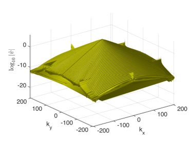
Figure 6: Solution to the NV equation (40) with $E=1$ for the initial data (41) with $c=-20$ and $\alpha=0.1$ for $t=1.4925$ on the left and the corresponding Fourier coefficients on the right.

The $L^{\infty}$ norm of $v$ and the $L^{2}$ norm of $v_{x}$ both indicate a blow-up as can be seen in Fig. 7. There appears to be a lump formation for $t\sim 1$ which then itself is unstable after a short time.

Figure 7: $L^{\infty}$ norm of the solution to the NV equation (40) with $E=1$ for the initial data (41) with $c=-20$ and $\alpha=0.1$ in dependence on time on the left and the $L^{2}$ norm of $v_{x}$ on the right.

To understand the mechanism of a potential blow-up, we perform a fit of $\ln C$ to $\gamma\ln(t^{*}-t)+\delta$, where $C$ is either the norm $||v||_{\infty}$ or the norm $||v_{x}||_{2}$, and where $t^{*}$ is the blow-up time and $\gamma$ and $\delta$ are constants. This fit is performed for the last 1000 time steps with the optimization algorithm [LRWW] which is distributed in Matlab as the command fminsearch. For the example in Fig. 6 we get for the norm $||v||_{\infty}$ the values $t^{*}=1.5125$, $\gamma=-0.99$ and $\delta=2.04$, and for the norm $||v_{x}||_{2}$ the values $t^{*}=1.5139$, $\gamma=-1.004$ and $\delta=-0.6261$. The quality of the fittings can be seen in Fig. 8, the fitting errors are of the order of $10^{-3}$. Note that the results do not change much if the fitting is done for the last 500 time steps. The compatibility between the found blow-up times shows the consistency of the fitting. The results indicate that the factor $L$ in (29) should be proportional to $\sqrt{t^{*}-t}$, i.e. the mechanism (33) with $\gamma_{1}=-1$. This would imply that the constant $a^{\infty}$ in (32) vanishes, and that the blow-up profile is the lump for $E=0$.

Figure 8: Fit of the norms in Fig. 7 to $\gamma\ln(t^{*}-t)+\delta$; the quantity $\Delta_{2}:=|\ln C-\gamma\ln(t^{*}-t)-\delta|$ for $C$ the $L^{\infty}$ norm of $v$ on the left and for $C$ the $L^{2}$ norm of $v_{x}$ on the right.

A similar picture is found for $E=0$, perturbations of a slow KdV soliton (small $|c|$) are stable, whereas perturbed faster solitons appear to blow up. We again consider initial data of the form (41), this time with $c=-10$ and $\alpha=0.1$. We use $N_{x}=N_{y}=2^{11}$ Fourier modes and $N_{t}=50000$ time steps. At $t\sim 1.47$, the relative energy conservation $H$ is no longer better than $10^{-3}$ and the results for larger times are ignored. The solution at a later time is shown in Fig. 9. As can be seen in the same figure on the right, there is a lack of resolution in the Fourier domain at this time.

Figure 9: Solution to the NV equation (40) with $E=0$ for the initial data (41) with $c=-10$ and $\alpha=0.1$ for $t=1.4775$ on the left and the corresponding Fourier coefficients on the right.

Both the $L^{\infty}$ norm and the $L^{2}$ norm of $v_{x}$ appear to explode as can be seen in Fig. 10. But in contrast to the case $E=1$ there does not appear to be ‘metastable’ structure at some intermediate time as in Fig. 7.

Figure 10: $L^{\infty}$ norm of the solution to the NV equation (40) with $E=0$ for the initial data (41) with $c=-10$ and $\alpha=0.1$ in dependence on time on the left and the $L^{2}$ norm of $v_{x}$ on the right.

We again fit various norms for the last 1000 time steps to $\gamma\ln(t^{*}-t)+\delta$ for constant $\gamma$ and $\delta$. For the example in Fig. 9 we get for the norm $||v||_{\infty}$ the values $t^{*}=1.4797$, $\gamma=-1.03$ and $\delta=0.05$, and for the norm $||v_{x}||_{2}$ the values $t^{*}=1.4785$, $\gamma=-0.91$ and $\delta=-1.77$. The quality of the fittings can be seen in Fig. 11, the fitting errors are of the order of $10^{-3}$. The results do not change much if the fitting is done for the last 500 time steps. The compatibility between the found blow-up times shows the consistency of the fitting. The results indicate once more a blow-up of the type (33) with $\gamma_{1}=-1$.

Figure 11: Fit of the norms in Fig. 10 to $\gamma\ln(t^{*}-t)+\delta$; the quantity $\Delta_{2}:=|\ln C-\gamma\ln(t^{*}-t)-\delta|$ for $C$ the $L^{\infty}$ norm of $v$ on the left and for $C$ the $L^{2}$ norm of $v_{x}$ on the right.

The blow-up mechanism that appears under the situations in Fig. 6 and Fig. 9 also implies that the profile of the self similar blow-up is given by a travelling wave solution of the NV equation for $E=0$, i.e. equation (32) with $a^{\infty}=0$. For $E=0$, two families of localized travelling wave solutions are known, the lumps (23) (or, more generally, (14) with $c=0$) and (26). Since the former vanish at the origin, their center of symmetry, they cannot be a candidate for a blow-up profile of the type observed here, blow-ups in isolated points. The lumps (26) are the only known candidates with the wanted behaviour. We choose $a=b=0$ (this just corresponds to a shift and rescaling of the solution). We determine the localization and value of the minima of the solution near the two peaks in Fig. 6 and Fig. 9. The quantity $L$ in (29) is fixed by fitting the rescaled soliton to the respective minima. In Fig. 12 we show the difference between the solution in Fig. 6 and the lump (26) rescaled according to (29) at each minimum on the left, and the corresponding figure for the situation of Fig. 9 on the right. It can be seen that these rescaled lumps catch the main profile. This is done in a much better way on the left than on the right, which indicates that the blow-up profile is indeed given by a dynamically rescaled lump (26). In the second case, it appears that we are not close enough to the blow-up to have an even better agreement since we ran out of resolution too early.

Figure 12: Difference between the numerical solution and a rescaled lump (26) with $a=b=0$ localized at the apparent blow-ups and rescaled according to (29); on the left for the situation for Fig. 6 and on the right for Fig. 9.

Note that we observe qualitatively the same behavior for $E=-1$ as for $E=0$ and $E=1$: perturbations of small enough KdV solitons are just radiated away and the soliton is thus stable. Larger solitons appear to be unstable against a blow-up. Since the results are very similar to what is shown above, we do not give details for this case.

5 Localized initial data

In this section we study localized initial data of the form

$$v(x,y,0)=\beta\exp(-x^{2}-y^{2}),$$ (42)

where $\beta$ is some real constant. Note that these initial data have finite mass in contrast to the KdV soliton treated in the previous section. Though we work numerically on $\mathbb{T}^{2}$ instead of $\mathbb{R}^{2}$ and thus always with finite masses, this different setting leads to some qualitative differences with respect to what was observed in the context of the KdV soliton.

5.1 The KPI limit: $E\gg 1$

We first consider the case $E=10$ for which NV should approach in some sense KP I. We use $N_{x}=N_{y}=2^{10}$ modes for $x,y\in 15[-\pi,\pi]$ and $N_{t}=1000$ time steps for $t\leq 0.2$. It can be seen in Fig.13 that the initial pulse with rotational symmetry is dispersed to infinity along three lines with an angle of 120 degrees between them. Note that the figures are very similar for positive values of $\beta$ in (42).

Figure 13: Solution of the NV equation (1a) with $E=10$ for the initial data (42) and $\beta=-10$; on the left the solution for $t=0.2$, on the right the $L^{\infty}$ norm of the solution in dependence of time.

The $L^{\infty}$ norm of the solution in the same figure indicates that the initial pulse is just dispersed on the studied time scales. This does not change if we run this example on longer scales of time and space. Thus it appears the initial data in this example are just dispersed to infinity without formation of a lump. We cannot exclude of course that a lump will appear at later times. But calculations for KPI in [KR2, DGK] show that lumps are difficult to observe in the context of localized initial data: there initial data with support on length scales of order $1/\epsilon$ were considered on time scales of the order $1/\epsilon$ with $\epsilon\ll 1$. In that case dispersive shock waves were observed, i.e., zones of rapid modulated oscillations in the solution. It seems that lumps can only appear in these examples for large times compared to the time where the dispersive shock forms. To access this in a reliable way, stronger computers would be needed than the ones used for the present work.

Thus it is not surprising that we do not see lumps in the solutions for the NV equation for initial data of the form (42) on the studied time scales. This does not change if we take even larger values of $E$ or larger values of $|\beta|$. Note, however, that the transition between the regime $E\approx 0$, where blow-up is possible, and the regime for large $E$, where a KPI type behavior is expected, is smooth. For very large values of $\beta$ ($\beta\sim-100$), there appears to be a blow-up.

5.2 The KPII limit: $E\ll-1$

For large negative values of $E$, the NV equation approaches the KPII equation. We show the solution for $E=-10$ for the initial data (42) with $\beta=-10$ in Fig. 14. It can be seen that the initial pulse is just radiated away to infinity. Again the 120 degree symmetry is observed for rotationally symmetric initial data. No stable structures appear in the evolution as can be seen also from the $L^{\infty}$ norm of the solution in the same figure. Since KPII has no lump solutions, and since its solutions are expected to exist globally in time, this is the expected behavior for this regime of NV. Note that in contrast to the same initial data for $E=10$ in Fig. 13, there are no oscillations orthogonal to the propagation direction of the pulses. The latter could lead to lumps if sufficient mass is present for $E\gg 1$, but such structures should not appear in the limit $-E\gg 1$. Instead the oscillations are here tangential to the triangular structure into which the initial pulse evolves.

Figure 14: Solution of the NV equation (1a) with $E=-10$ for the initial data (42) and $\beta=-10$; on the left the solution for $t=0.2$, on the right the $L^{\infty}$ norm of the solution in dependence of time.

If we take initial data without rotational symmetry, the solution will not have this 120 degree symmetry, but its propagation will follow the 120 degree pattern. This can be seen in Fig. 15 for the initial data $v(x,y,0)=\exp(-x^{2}-5y^{2}-3xy)$ which are not rotationally symmetric even for $|x|,|y|\to\infty$. The computation is carried out for $x\in 10[-\pi,\pi]$ and $y\in 7[-\pi,\pi]$ with $N_{x}=N_{y}=2^{10}$ Fourier modes and $N_{t}=10^{3}$ time steps for $t\leq 0.06$.

Figure 15: Solution of the NV equation (1a) for the initial data $v(x,y,0)=\exp(-x^{2}-5y^{2}-3xy)$ and $E=-10$ for $t=0.06$.

5.3 Intermediate values of $E$

For $E=0$, the solution to the NV equation for the initial data (42) with $\beta=-1$ appears to be global in time. The computation is done with $N_{x}=N_{y}=2^{10}$ Fourier modes for $[x,y]\in 20[-\pi,\pi]^{2}$. The resulting solution can be seen in Fig. 16. It appears to be just dispersed away towards infinity along the 120 degree lines. This is confirmed by the $L^{\infty}$ norm of the solution on the right of Fig. 16 which appears to decrease monotonically.

Figure 16: Solution of the NV equation (1a) for the initial data (42) and $\beta=-1$ for $E=0$; on the left the solution for $t=1$, on the right the $L^{\infty}$ norm of the solution in dependence of time.

However, for $E=0$ and the initial data (42) with $\beta=-10$, there appears to be a blow-up in finite time. The code is run for $[x,y]\in 5[-\pi,\pi]\times[-\pi,\pi]$ with $N_{x}=N_{y}=2^{11}$ Fourier modes and $N_{t}=10^{5}$ time steps for $t\leq 0.14$. The code is stopped at $t=0.1365$ where the relative conservation of energy $H$ drops below $10^{-3}$. The solution at this time is shown in Fig.17. It can be seen that, because of the rotational symmetry of the initial data, the solution shows the 120 degree symmetry. Thus the blow-up appears to happen in 3 points at the same time. The Fourier coefficients at the final time on the right of Fig. 17 indicate once more that resolution in $t$ appears to lack in these blow-ups before this happens in the spatial coordinates.

Figure 17: Solution of the NV equation (40) for the initial data (42) and $\beta=-10$ for $E=0$; on the left the solution for $t=0.1365$ close to a blow-up, on the right the modulus of the Fourier coefficients at the same time.

Once more both the $L^{\infty}$ norm of $v$ and the $L^{2}$ norm of $v_{x}$ indicate a blow-up as can be seen in Fig. 18.

Figure 18: $L^{\infty}$ norm of the solution to the NV equation (40) with $E=0$ for the initial data (42) with $\beta=-10$ in dependence on time on the left and the $L^{2}$ norm of $v_{x}$ on the right.

To understand the mechanism of a potential blow-up, we again perform a fit of $\ln C$ to $\gamma\ln(t^{*}-t)+\delta$, where $C$ is either the norm $||v||_{\infty}$ or the norm $||v_{x}||_{2}$, $t^{*}$ is the blow-up time and $\gamma$ and $\delta$ are constants. This fit is performed for the last 500 time steps (the results are very similar for the last 100 time steps) with the optimization algorithm [LRWW]. For the example in Fig. 18 we get for the norm $||v||_{\infty}$ the values $t^{*}=0.1369$, $\gamma=-0.997$ and $\delta=-0.902$, and for the norm $||v_{x}||_{2}$ the values $t^{*}=0.1369$, $\gamma=-0.983$ and $\delta=-2.667$. The quality of the fittings can be seen in Fig. 19, the fitting errors are of the order of $10^{-4}$. The compatibility between the found blow-up times shows the consistency of the fitting. The results again indicate that the factor $L$ in (29) should be proportional to $\sqrt{t^{*}-t}$, as in (33) with $\gamma_{1}=-1$ which gives some indication that this is indeed the generic blow-up mechanism to be observed in NV solutions.

Figure 19: Fit of the norms in Fig. 18 to $\gamma\ln(t^{*}-t)+\delta$; the quantity $\Delta_{2}:=|\ln C-\gamma\ln(t^{*}-t)-\delta|$ for $C$ the $L^{\infty}$ norm on the left and for $C$ the $L^{2}$ norm of $v_{x}$ on the right.

Again this blow-up mechanism implies that the profile of the self similar blow-up is given by a travelling wave solution of the NV equation for $E=0$. We determine the localization and value of the minima of the solution near the three peaks in Fig. 17. The quantity $L$ in (29) is fixed by fitting the rescaled soliton to the respective minima. Note that the 120 degree symmetry is not exactly observed at the recorded time, thought it appears to be an attractor for the asymptotic state of the solution. The fitting, however, is performed for each point separately. In Fig. 20 we show the difference between the solution in Fig. 17 and the lump (26) rescaled according to (29) at each minimum. It can be seen that these rescaled lumps catch the main profile (the difference is smaller than the solution by more than an order of magnitude), but that we are, as expected, not close enough to the blow-up to have an even better agreement.

Figure 20: Difference of the NV solution in Fig. 17 and three lumps (26) rescaled according to (29) at each minimum.

Note that very similar behavior is observed for $E=\pm 1$ as for $E=0$ which is why we do not discuss these cases in more detail: initial data of sufficiently small $L^{2}$ norm are just radiated away, whereas initial data of large enough $L^{2}$ norm blow-up in finite time.

6 Conclusion

In the present paper we have studied numerically the evolution under NV dynamics of localized initial data and of perturbed KdV solitons.

For large values of $E$ the NV equation behaves qualitatively as the KPI equation: sufficiently small KdV solitons appear to be stable under localized perturbations. Larger solitons appear to be unstable against the formation of lump-like structures which resemble the Grinevich-Zakharov traveling wave solutions to NV at $E>0$. The long time behaviour of NV solutions for $E\gg 1$ for localized initial data is given by lumps and radiation. The results can be summarized in the following conjecture:

Conjecture 1.

Let $E\gg 1$.
- The KdV soliton (39) for small $a$ is stable under NV dynamics.
- The KdV soliton (39) for large $a$ is unstable under NV dynamics. Asymptotically for $t$ large, smaller KdV solitons, lumps and radiation will appear.
- Localized initial data will develop under NV dynamics for $t$ large into radiation and lumps.

For $E\ll-1$, the NV equation behaves qualitatively as the KPII equation: the KdV soliton appears to be stable, and localized initial data will be just radiated away:

Conjecture 2.

Let $E\ll-1$.
- The KdV soliton (39) is stable under NV dynamics.
- Localized initial data will be radiated away to infinity under NV dynamics for $t$ large.

For small values of $|E|$, KdV solitons of sufficiently small size are again stable. Larger perturbed solitons will form a blow-up at a finite time. Localized initial data of sufficiently small $L^{2}$ norm are dispersed away as time goes to infinity. However, when the initial data have a large enough $L^{2}$ norm there appears to be a blow-up at finite time. We have not observed the formation of lumps from localized initial data. However, based on our knowledge about related $2d$ integrable equations, we conjecture that it may be due to the fact that the time scales that we consider are not large enough. The appearance of oscillations transversal to the direction of propagation of the initial pulse at $E>0$ could be a potential mechanism for lump formation at larger times. The results can be summarized in the following conjecture (note that numerical studies of a blow-up are always challenging and have to be taken with a grain of salt):

Conjecture 3.

Let $|E|\ll 10$.
- The KdV soliton (39) for small $a$ is stable under NV dynamics.
- The KdV soliton (39) for large $a$ is unstable under NV dynamics against an $L^{\infty}$ blow-up in finite time.
- NV solutions corresponding to localized initial data of sufficiently small $L^{2}$ norm are global in time. Localized initial data of sufficiently large $L^{2}$ norm will blow-up in finite time.
- A blow-up at time $t^{*}$ is self similar according to the scaling (29) for $t\sim t^{*}$,

$$v\sim\frac{1}{L^{2}}Q\left(\frac{z-z^{*}}{L}\right),\quad L=\sqrt{t^{*}-t},$$ (43)

where $z^{*}$ is the location of the blow-up which appears to be finite, and where $Q$ is the lump (26).

The numerical results indicate that the lumps of NV are stable for $E\gg 1$ since they appear in the perturbations of the KdV soliton. Since this is not the case for $E\sim 0$, it can be concluded that they are unstable against blow-up in this case. A direct study of this important question is, however, not possible with the wanted accuracy by the Fourier methods applied in this paper. This is due to the fact that rational functions because of their slow fall-off to infinity are not well approximated by a periodic continuation of their restriction to a finite computational domain, in contrast to the Schwartz functions studied here. The same is also true for the exact blow-up solutions (14) and (13). For such functions, an approximation via polynomials, see [BK] and references therein, would be much more efficient. The interesting question in this context would be whether the blow-up of the exact solutions which is as the blow-up (35) is unstable whereas the generic one is as observed here given by (33). Such a situation is known from nonlinear Schrödinger equations, see for instance the discussion in [Sul] and references therein. This will be the subject of further research.

References

- [A] Angelopoulos Y. Well-posedness and ill-posedness results for the Novikov-Veselov equation. Comm. Pure Appl. Analysis 15(3), 727-760 (2016)
- [BK] Birem M., Klein C. Multidomain spectral method for Schrödinger equations. Adv. Comp. Math. 42(2), 395–423 DOI 10.1007/s10444-015-9429-9 (2016)
- [Ch] Chang J.-H. The Gould-Hopper polynomials in the Novikov-Veselov equation. J. Math. Phys. 52(9), 092703 (2011)
- [CM] Cox S., Matthews P. Exponential time differencing for stiff systems. Journal of Computational Physics. 176 , 430-455 (2002)
- [C.et.al] Croke R., Mueller J.L., Music M., Perry P., Siltanen S., Stahel A. The Novikov-Veselov Equation: Theory and Computation. Contemporary Mathematics. 635, 25-70 (2015)
- [Cr] Croke R., Mueller J.L., Stahel A. Transverse instability of plane wave soliton solutions of the Novikov-Veselov equation. Contemporary Mathematics. 635, 71-89 (2015)
- [DGK] Dubrovin B., Grava T., Klein C. On critical behaviour in generalized Kadomtsev–Petviashvili equations. Physica D. doi:10.1016/j.physd.2016.01.011 (2016)
- [F] Ferapontov E.V. Stationary Veselov-Novikov equation and isothermally asymptotic surfaces in projective differential geometry. Diff. Geom. and Appl. 11(2), 117-128 (1999)
- [FN] Francoise J.–P., Novikov R.G. Rational solutions of KdV–type equations in dimension and –body problems on the line. C.R. Acad. Sci. Paris Sér. I Math. 314(2), 109–113 (1992) (in French)
- [G] Grinevich P.G. Scattering transformation at fixed non-zero energy for the two-dimensional Schrödinger operator with potential decaying at infinity. Russ. Math. Surv. 55(6), 1015–1083 (2000)
- [KT] Kassam A.-K., Trefethen L. Fourth-order time-stepping for stiff PDEs. SIAM J. Sci. Comput. 26, 1214–1233 (2005)
- [K1] Kazeykina A.V. A large time asymptotics for the solution of the Cauchy problem for the Novikov-Veselov equation at negative energy with non-singular scattering data. Inverse Problems, 28(5), 055017 (2012).
- [K2] Kazeykina A.V. Absence of solitons with sufficient algebraic localization for the Novikov-Veselov equation at nonzero energy. Funct. Anal. Appl., 48(1), 24-35 (2014)
- [KN1] Kazeykina A.V., Novikov R.G. A large time asymptotics for transparent potentials for the Novikov–Veselov equation at positive energy. J. Nonlinear Math. Phys. 18(3), 377-400 (2011).
- [KN2] Kazeykina A.V., Novikov R.G. Large time asymptotics for the Grinevich–Zakharov potentials. Bulletin des Sciences Mathématiques. 135, 374-382 (2011)
- [KN3] Kazeykina A.V., Novikov R.G. Large time asymptotics for the Grinevich–Zakharov potentials. Bulletin des Sciences Mathématiques. 135, 374-382 (2011)
- [KM] Kazeykina A., Muñoz C.: Dispersive estimates for rational symbols and local well-posedness of nonzero energy Novikov-Veselov equation. Journal of Funct. Anal., 270(5), 1744-1791 (2016)
- [KM2] Kazeykina A., Muñoz C. Dispersive estimates for rational symbols and local well-posedness of the nonzero energy NV equation. II. arxiv.org:1603.06600
- [K] Klein C. Fourth order time-stepping for low dispersion Korteweg-de Vries and nonlinear Schrödinger equation. ETNA. 29, 116–135 (2008)
- [KP1] Klein C., Peter R. Numerical study of blow-up in solutions to generalized Korteweg-de Vries equations. Physica D. 304–305, 52–78 (2015)
- [KP2] Klein C., Peter R. Numerical study of blow-up in solutions to generalized Kadomtsev-Petviashvili equations, Discr. Cont. Dyn. Syst. B 19(6), 1689–1717 (2014)
- [KR] Klein C., Roidot K. Fourth order time-stepping for Kadomtsev-Petviashvili and Davey-Stewartson equations. SIAM J. Sci. Comput. 33(6), 3333–3356 (2011)
- [KR2] Klein C., Roidot K. Numerical study of shock formation in the dispersionless Kadomtsev-Petviashvili equation and dispersive regularizations, Physica D. 265, 1–25 (2013)
- [KS1] Klein C., Saut J.-C. IST versus PDE: Numerical study of blow up and stability of solutions of generalized Kadomtsev-Petviashvili equations, J. Nonl. Sci. 22(5), 763-811 (2012)
- [KS2] Klein C., Saut J.-C. IST versus PDE: a comparative study. Hamiltonian Partial Differential Equations and Applications, Vol. 75 of the series Fields Institute Communications, 383-449 (2015)
- [KM3] Konopelchenko B., Moro A. Integrable equations in nonlinear geometrical optics. Studies in Applied Mathematics. 113(4), 325-352 (2004)
- [LRWW] Lagarias J.C., Reeds J.A, Wright M.H., Wright P.E. Convergence properties of the Nelder-Mead simplex method in low dimensions. SIAM Journal of Optimization. 9, 112–147 (1999)
- [M] Manakov S.V. The inverse scattering method and two-dimensional evolution equations. Uspekhi Mat. Nauk. 31(5), 245–246 (1976) (in Russian)
- [MMR] Martel Y., Merle F., Raphael P. Blow up for the critical gKdV equation I: dynamics near the solitary wave. Acta Math 212(1), 59–140 (2014)
- [MP] Music M., Perry P. Global solutions for the zero-energy Novikov-Veselov equation by inverse scattering. arxiv:1502.02632 (2015)
- [Na] Nachman A.I. Global uniqueness for a two-dimensional inverse boundary value problem. Annals of Mathematics. 143, 71-96 (1995)
- [N] Novikov R. G. The inverse scattering problem on a fixed energy level for the two-dimensional Schrödinger operator. J. Funct. Anal. 103(2), 409-463 (1992)
- [N2] Novikov R.G. Absence of exponentially localized solitons for the Novikov–Veselov equation at positive energy. Physics Letters A. 375, 1233-1235 (2011)
- [NV1] Novikov S.P., Veselov A.P. Finite-zone, two-dimensional, potential Schrödinger operators. Explicit formula and evolutions equations. Dokl. Akad. Nauk SSSR. 279, 20–24 (1984), translation in Sov. Math. Dokl. 30, 588–591 (1984)
- [NV2] Novikov S.P., Veselov A.P. Finite-zone, two-dimensional Schrödinger operators. Potential operators. Dokl. Akad. Nauk SSSR. 279, 784–788 (1984), translation in Sov. Math. Dokl. 30, 705–708 (1984)
- [RT] Rousset F., Tzvetkov N. Transverse nonlinear instability for two-dimensional dispersive models. Ann. Inst. Henri Poincaré, Anal. Non Linéaire. 26, 477–496 (2009)
- [P] Perry P. Miura maps and inverse scattering for the Novikov-Veselov equation. Anal PDE 7(2), 311-343 (2014)
- [Sch] Schmelzer T. The fast evaluation of matrix functions for exponential integrators. PhD thesis, Oxford University (2007)
- [Sul] Sulem C., Sulem P.L. The nonlinear Schrödinger equation. Applied Mathematical Sciences, Springer, Berlin (1999)
- [TT] Taimanov I. A., Tsarev, S. P. Blowing up solutions of the Veselov-Novikov equation, (Russian) Dokl. Akad. Nauk. 420(6), 744–745 (2008); translation in Dokl. Math. 77(3), 467–468 (2008)
- [Zak] Zakharov V.E. Instability and nonlinear oscillations of solitons. JETP Lett. 22, 172–173 (1975)