S-duality invariant perturbation theory
improved by holography

Abstract

We study anomalous dimensions of unprotected low twist operators in the four-dimensional $SU(N)$ $\mathcal{N}=4$ supersymmetric Yang-Mills theory. We construct a class of interpolating functions to approximate the dimensions of the leading twist operators for arbitrary gauge coupling $\tau$. The interpolating functions are consistent with previous results on the perturbation theory, holographic computation and full S-duality. We use our interpolating functions to test a recent conjecture by the $\mathcal{N}=4$ superconformal bootstrap that upper bounds on the dimensions are saturated at one of the duality-invariant points $\tau=i$ and $\tau=e^{i\pi/3}$. It turns out that our interpolating functions have maximum at $\tau=e^{i\pi/3}$, which are close to the conjectural values by the conformal bootstrap. In terms of the interpolating functions, we draw the image of conformal manifold in the space of the dimensions. We find that the image is almost a line despite the conformal manifold is two-dimensional. We also construct interpolating functions for the subleading twist operator and study level crossing phenomenon between the leading and subleading twist operators. Finally we study the dimension of the Konishi operator in the planar limit. We find that our interpolating functions match with numerical result obtained by Thermodynamic Bethe Ansatz very well. It turns out that analytic properties of the interpolating functions reflect an expectation on a radius of convergence of the perturbation theory.

HRI/ST/1601, TIFR/TH/16-18, WIS/06/16-JUN-DPPA

1 Introduction

In the last two decades, there has been huge progress in understanding the four-dimensional $\mathcal{N}=4$ supersymmetric Yang-Mills theory (SYM). The $\mathcal{N}=4$ SYM is supposed to have many special properties such as superconformal symmetry [1, 2, 3, 4, 5], UV finiteness [5, 6, 7], S-duality [8, 9, 10, 11, 12], integrability [13, 14], dual conformal symmetry [15] and so on. The $\mathcal{N}=4$ SYM also provides the canonical example of the AdS/CFT correspondence [16, 17, 18], where the $\mathcal{N}=4$ SYM is dual to type IIB superstring on $AdS_{5}\times S^{5}$. While the AdS/CFT correspondence has stimulated our understanding on the $\mathcal{N}=4$ SYM and vice versa, most of the progress is based on weak coupling perturbation theory, planar limit or protected observables.

Recently it has turned out that the conformal bootstrap approach [19, 20, 21, 22] is very powerful tool also for the $\mathcal{N}=4$ SYM [23] (see also [28, 29, 30, 31]). Indeed the $\mathcal{N}=4$ superconformal bootstrap [23] gives strong constraints on dimensions of unprotected leading twist operators with various spins, which are $SU(4)_{R}$ singlets and non-BPS primary operators belonging to long representation of the $\mathcal{N}=4$ superconformal group. The leading twist operators in the $\mathcal{N}=4$ SYM at classical level are the so-called twist-two operators defined by

$$\mathcal{O}_{M}={\rm Tr}\phi^{I}D^{M}\phi^{I},\qquad M=0,2,4,\cdots,$$ (1.1)

where $\phi^{I}$ is the adjoint scalar. The $\mathcal{N}=4$ superconformal bootstrap finds rigorous bounds on the dimensions within numerical errors, which are fully non-perturbative even for finite $N$ and independent of the complex gauge coupling $\tau=\frac{\theta}{2\pi}+\frac{4\pi i}{g_{\rm YM}^{2}}$. The authors in [23] have also conjectured that the upper bounds on the dimensions are saturated at either $\tau=i$ or $\tau=e^{i\pi/3}$, which are the duality invariant points under $\mathbf{S}$-transformation and $(\mathbf{T}\cdot\mathbf{S})$-transformation, respectively.

Main purpose of this paper is to study the dimensions of the leading twist operators in the $SU(N)$ $\mathcal{N}=4$ SYM by a completely different approach. We find approximate formula of the dimensions by resumming the perturbative data with help of the S-duality [8, 9, 10, 11, 12] and AdS/CFT correspondence [16, 17, 18]. We approximate the dimensions through interpolating functions which interpolates between two perturbative expansions around two different points in parameter space. The standard approach is to apply (two-point) Padé approximation, which is a rational function encoding the two expansions up to some orders. Recently Sen constructed another type of interpolating function, which has the form of a Fractional Power of Polynomial (FPP) [32]. A more general form of the interpolating function with the form of Fractional Powers of Rational function (FPR) has been constructed out by one of the current authors [33]. It has turned out that these interpolating functions usually provide better approximations than each perturbative expansion in intermediate regime of the parameter. See [32, 33, 34, 35, 36, 37, 38] for various applications.

In this paper, we construct a class of interpolating functions to approximate the anomalous dimensions, which are consistent with known results on the perturbation theory, holographic computation and full S-duality $SL(2,\mathbb{Z})$. In other words, our modular invariant interpolating functions reproduce the correct weak coupling expansion and large ’t Hooft coupling limit in the planar limit. Such attempt was initiated in [41], which has constructed interpolating functions invariant under one particular element of $SL(2,\mathbf{Z})$ either $\mathbf{S}$ or $(\mathbf{T}\cdot\mathbf{S})$-transformations. After a while, Alday and Bissi constructed a class of interpolating functions [37], which is similar to FPP [32] but invariant under all elements of $SL(2,\mathbf{Z})$. Here we construct a new class of interpolating functions by combining the ideas of FPR [33] and Alday-Bissi [37], and further imposing a consistency with the previous holographic results.

Our interpolating functions give predictions for arbitrary values of $N$ and the complex gauge coupling $\tau$. We compare our result with the recent results by the $\mathcal{N}=4$ superconformal bootstrap and test the conjecture that the upper bounds on the dimensions are saturated at one of the duality-invariant points $\tau=i$ and $\tau=e^{i\pi/3}$. As a conclusion we find that when we expect reasonable approximation by the interpolating functions, the interpolating functions have their maximal values at $\tau=e^{i\pi/3}$, close to the conjectural values of the $\mathcal{N}=4$ superconformal bootstrap.

In terms of the interpolating functions, we also study an image of conformal manifold in the space of the dimensions of the leading twist operators. We find that despite varying the coupling $\tau$ in the (real) two-dimensional region, the image is a very narrow line, which is almost one-dimensional. The narrow line is almost straight for $N=2$ as in the result by different interpolating functions [41] while it is somewhat curved for $N\geq 3$ contrary to [41].

We also construct interpolating functions for the subleading twist operator and study level crossing phenomenon between the leading and subleading twist operators. We use the terminology “level crossing” in the following two senses. As we increase the coupling, the dimensions of the leading and subleading operators approach each other with two possibilities. Firstly, there is no operator mixing due to additional protected symmetries and their dimensions cross over. Secondly, operator mixing occurs and the dimensions of new eigenstates repel. We refer to the both as level crossing. We check that the interpolating functions for the leading and subleading twist operators with spin-0 do not cross each other for finite $N$. Namely the level crossing in the first sense does not occur for finite $N$. For large but finite $N$, we observe that the dimension of the leading twist operator becomes very close to the subleading one around $\tau=i$ and $\tau=e^{\pi i/3}$. This implies that the level crossing in the second sense occurs for large but finite $N$.

We also study the dimension of the Konishi operator in the planar limit. We construct interpolating functions consistent with the weak coupling expansion and holographic computation. We compare our result with numerical data obtained by Thermodynamic Bethe Ansatz (TBA) and find that our interpolating functions match very well with the TBA result. We also discuss that analytic property of the interpolating function reflects expectations on radius of convergence from the weak coupling perturbation theory.

This paper is organized as follows. In section 2 we briefly explain the previous results obtained by the weak coupling perturbation theory, holographic computation, and superconformal bootstrap. In section 3 we begin with introducing interpolating functions constructed previously. Then we construct our interpolating functions for the anomalous dimensions, which are consistent with the known results on the weak coupling perturbation theory, holographic results and full S-duality. Finally we discuss which of our interpolating functions would give the best approximation. Section 4 is the main section of this paper. We compare our results with the recent results by the $\mathcal{N}=4$ superconformal bootstrap. We also draw the image of the conformal manifold in the space of the dimensions of the leading twist operators and study the level crossing phenomenon between the leading and subleading twist operators for finite $N$. In section 5 we study the dimension of the Konishi operator in the planar limit. Section 6 is devoted to conclusion and discussions.

2 Previous results on leading twist operators

In this paper we mainly study the dimensions of the leading twist operators in the 4d $SU(N)$ $\mathcal{N}=4$ SYM by using the technique of interpolating functions. Before introducing the interpolating functions, we review some relevant previous results know in the literature.

The leading twist operators under consideration are $SU(4)_{R}$ singlet and non-BPS primary operators belonging to long representation of the $\mathcal{N}=4$ superconformal group. At classical level, these operators are so-called twist-two operators:

$$\mathcal{O}_{M}={\rm Tr}\phi^{I}D^{M}\phi^{I},$$

where $\phi^{I}$ are the adjoint scalars in the $\mathcal{N}=4$ SYM and $I$ is an index in the $\bf{6}$ of $SU(4)_{R}$. The leading twist operator has the dimension $(2+M)$ classically but receives quantum corrections:

$$\Delta_{M}(\tau,N)=2+M+\gamma_{M}(\tau,N),$$ (2.1)

depending on the complex gauge coupling

$$\tau=\frac{\theta}{2\pi}+\frac{i}{g},\quad{\rm with}\ \ g=\frac{g_{\rm YM}^{2}}{4\pi}.$$ (2.2)

It is known that its weak coupling perturbative expansion is independent of $\theta$ while non-perturbative corrections depend on $\theta$ generically. It is expected that the $\mathcal{N}=4$ SYM possesses the S-duality [8, 9, 10, 11, 12] described by the $SL(2,\mathbb{Z})$ transformation

$$\mathbf{h}\cdot\tau=\frac{a\tau+b}{c\tau+d},\quad{\rm where}\ ad-bc=1,\ a,b,c,d\in\mathbb{Z},$$ (2.3)

which is a combination of $\mathbf{S}$- and $\mathbf{T}$-transformations:

$$\mathbf{S}\cdot\tau=-\frac{1}{\tau},\quad\mathbf{T}\cdot\tau=\tau+1.$$ (2.4)

Note that there are two special values of $\tau$:

$$\tau=\tau_{S}=i,\quad\tau=\tau_{TS}=e^{i\pi/3},$$ (2.5)

which are invariant under $\mathbf{S}$-transformation and $(\mathbf{T}\cdot\mathbf{S})$-transformation, respectively. In this paper we assume $SL(2,\mathbb{Z})$ invariance of the dimensions of the leading-twist operators:

$$\Delta_{M}(\mathbf{h}\cdot\tau)=\Delta_{M}(\tau),\quad\gamma_{M}(\mathbf{h}\cdot\tau)=\gamma_{M}(\tau),$$ (2.6)

and construct the interpolating functions based on this assumption.

2.1 Weak coupling expansion

In perturbative regime, the leading twist operator is the twist-two operator $\mathcal{O}_{M}$ (1.1), which is the Konishi operator especially for $M=0$ (see e.g. [42, 44]). The anomalous dimension of the twist-two operator has been computed up to four-loop for $M=0,2$ and three-loop for $M=4$ in the weak coupling perturbation theory [48, 49, 50, 51, 52, 53, 54]:

$$\gamma_{0}(\tau,N) = \frac{3N}{\pi}g-\frac{3N^{2}}{\pi^{2}}g^{2}+\frac{21N^{3}}{4\pi^{3}}g^{3}+\Biggl{[}-39+9\zeta(3)-45\zeta(5)\left(\frac{1}{2}+\frac{6}{N^{2}}\right)\Biggr{]}\frac{N^{4}g^{4}}{4\pi^{4}}+\mathcal{O}(g^{5}),\mbox{$$}$$

$$\gamma_{2}(\tau,N) = \frac{25N}{6\pi}g-\frac{925N^{2}}{216\pi^{2}}g^{2}+\frac{241325N^{3}}{31104\pi^{3}}g^{3}\mbox{$$}$$

$$+\Biggl{[}-\frac{8045275}{2187}+\frac{114500\zeta(3)}{81}-\frac{25000\zeta(5)}{9}+\frac{8400+28000\zeta(3)-100000\zeta(5)}{3N^{2}}\Biggr{]}\frac{N^{4}g^{4}}{(4\pi)^{4}}\mbox{$$}$$

$$+\mathcal{O}(g^{5}),\mbox{$$}$$

$$\gamma_{4}(\tau,N) = \frac{49N}{10\pi}g-\frac{45619N^{2}}{9000\pi^{2}}g^{2}+\frac{300642097N^{3}}{32400000\pi^{3}}g^{3}+\mathcal{O}(g^{4}).$$ (2.7)

These data will be used to construct our interpolating functions in subsequent sections.

2.2 Supergravity limit

The $\mathcal{N}=4$ SYM is expected to be dual to type IIB supergravity on $AdS_{5}\times S^{5}$ at large ’t Hooft coupling $\lambda=gN$ [16, 17, 18] in the planar limit. In the planar limit, the anomalous dimension of the twist-two operator $\mathcal{O}_{M}$ (1.1) typically grows as $\sim\lambda^{1/4}$ [17] and the twist-two operator is no longer leading twist operator for large ’t Hooft coupling. The leading twist operator in the supergravity limit is a double trace operator which has a schematic form

$${\rm tr}(\phi^{(i}\phi^{j)})D^{M}{\rm tr}(\phi^{(i}\phi^{j)}),$$ (2.8)

where ${\rm tr}(\phi^{(i}\phi^{j)})$ is symmetric traceless part of ${\rm tr}(\phi^{i}\phi^{j})$ and chiral primary operator belonging to $\mathbf{20^{\prime}}$ representation of $SU(4)_{R}$. The double trace operator (2.8) is not protected in general but the large-$N$ factorization implies that the dimension becomes the sum of the protected single trace operators and therefore protected in the planar limit. One can compute the anomalous dimension of the double trace operator (2.8) by the supergravity [55, 56, 57] and then the one of the leading twist operator in the supergravity limit is

$$\gamma_{0}^{\rm SUGRA}(N)=2-\frac{16}{N^{2}},\quad\gamma_{2}^{\rm SUGRA}(N)=2-\frac{4}{N^{2}},\quad\gamma_{4}^{\rm SUGRA}(N)=2-\frac{48}{25N^{2}}.$$ (2.9)

Note that the first terms are easily understood by the large-$N$ factorization.

2.3 The $\mathcal{N}=4$ superconformal bootstrap

In the past few years the $\mathcal{N}=4$ superconformal bootstrap approach [23] has obtained a relatively satisfying upper bounds on the dimensions of the unprotected leading twist operators by studying the four-point function (see also [28, 29, 30])

$$\langle\mathcal{O}_{\bf 20^{\prime}}^{I_{1}}(x_{1})\mathcal{O}_{\bf 20^{\prime}}^{I_{2}}(x_{2})\mathcal{O}_{\bf 20^{\prime}}^{I_{3}}(x_{3})\mathcal{O}_{\bf 20^{\prime}}^{I_{4}}(x_{4})\rangle,$$ (2.10)

where $\mathcal{O}_{\bf 20^{\prime}}^{I}$ is a superconformal primary scalar operator of dimension two in energy-momentum tensor multiplets transforming as $\mathbf{20^{\prime}}$ representation in $SU(4)_{R}$. The $\mathcal{N}=4$ superconformal symmetry allows us to describe the four-point function in terms of the $\mathcal{N}=4$ superconformal block [58, 55, 59, 60].

	$SU(2)$	$SU(3)$	$SU(4)$
Strict upper bound on $\gamma_{0}$	1.05	1.38	1.59
Corner value on $\gamma_{0}$	0.93	1.24	1.47
Strict upper bound on $\gamma_{2}$	1.32	1.66	1.80
Corner value on $\gamma_{2}$	1.28	1.60	1.75
Strict upper bound on $\gamma_{4}$	1.55	1.80	1.89
Corner value on $\gamma_{4}$	1.53	1.79	1.88

Table 1: Bounds and corner values from Superconformal bootstrap [23].

In [23] the upper bounds on the dimensions of the leading twist operators with spin-0, 2 and 4, were obtained which are rigorous within numerical errors. Exclusion plots on the anomalous dimensions $(\gamma_{0},\gamma_{2},\gamma_{4})$ are presented in fig.1 of [23]. While the shape of not-excluded region roughly looks like a cube, its precise shape is complicated function of $(\gamma_{0},\gamma_{2},\gamma_{4})$. The “bound” values are listed in table 1 for each maximal value of $(\gamma_{0},\gamma_{2},\gamma_{4})$ in the not-excluded region.

The “bound” values in table 1 are somewhat conservative. This is because if actual values of $(\gamma_{0},\gamma_{2})$ were not equal to the bound values in table 1 (namely smaller than the bound values) for example, then possible value of $\gamma_{4}$ would generically be more strongly constrained. Hence we might have better estimates from fig.1 of [23] than the bound values in table 1. The authors in [23] have conjectured that this better estimate is given by the value at the corner of the cube-like region and that this is saturated by values of $\gamma_{M}$ at one of duality invariants points $\tau=\tau_{S}$ or $\tau=\tau_{TS}$. This conjecture essentially claims the following two things:

1. The corner value obtained by the conformal bootstrap is saturated by the maximal value of $\gamma_{M}(\tau,N)$.

2. The maximal value of $\gamma_{M}(\tau,N)$ in the physical region of $\tau$ is given by $\tau=\tau_{S}$ or $\tau=\tau_{TS}$.

The first point of this conjecture is closely related to whether the constraints from the conformal bootstrap is sufficiently strong or not. Namely, the upper bound of the bootstrap is greater than all the possible values of the anomalous dimension in general and may have a gap from the maximal value in principle. However, if the upper bound is maximally strong, then there is no such gap and the upper bound is the same as the maximal value though it is currently unclear if this is true. Regarding the second point, we do not know a priori which value of the coupling realizes the maximal value but it is natural to expect that such special thing happens in some special values in the $\tau$-space, which are only the duality invariant points $\tau=\tau_{S}$ and $\tau=\tau_{TS}$ to our knowledge. Main purpose of this paper is to test the conjecture by using the interpolating functions.

3 Interpolating functions

In this section we introduce some classes of interpolating functions constructed in the literature [32, 41, 37, 33] and then in the remaining part of this section we construct new class of interpolating functions for the anomalous dimensions of the leading twist operators. We impose the following conditions to the interpolating functions:

1. Real for ${\rm Im}\tau\geq 0$.

2. Small-$g$ expansion agrees with the weak coupling expansion of $\gamma_{M}(g)$ up to certain order.

3. Invariant under the full $SL(2,\mathbb{Z})$ duality (2.3): $\gamma_{M}(\mathbf{h}\cdot\tau)=\gamma_{M}(\tau)$.

4. Reproduce the holographic result in the planar limit at large ’t Hooft coupling.

3.1 Interpolating functions without $S$-duality (FPR)

Before considering the S-duality invariant interpolating functions, we introduce usual interpolating functions, which can be applied to problems without S-duality. Suppose that we would like to approximate a function $F(g)$, which has the small-$g$ expansion around $g=0$ and large-$g$ expansion around $g=\infty$ taking the forms

$$F(g)=g^{a}(s_{0}+s_{1}g+s_{2}g^{2}+\cdots)=g^{b}(l_{0}+l_{1}g^{-1}+l_{2}g^{-2}+\cdots).$$ (3.1)

The author in [33] constructed the following type of interpolating function for the function $F(g)$:

$$F_{m,n}^{(\alpha)}(g)=s_{0}g^{a}\Biggl{[}\frac{1+\sum_{k=1}^{p}c_{k}g^{k}}{1+\sum_{k=1}^{q}d_{k}g^{k}}\Biggr{]}^{\alpha},$$ (3.2)

where

$$p=\frac{1}{2}\left(m+n+1-\frac{a-b}{\alpha}\right),\quad q=\frac{1}{2}\left(m+n+1+\frac{a-b}{\alpha}\right).$$ (3.3)

Here the coefficients $c_{k}$ and $d_{k}$ are determined such that power series expansions around $g=0$ and $g=\infty$ agree with the ones of $F(g)$ up to $\mathcal{O}(g^{a+m+1})$ and $\mathcal{O}(g^{b-n-1})$, respectively. By construction, the interpolating function reproduces both the small-$g$ and large-$g$ expansions of $F(g)$. Since this interpolating function is described by Fractional Power of Rational function, we call this FPR. Note that we need

$$p,q\in\mathbb{Z}_{\geq 0},$$ (3.4)

which leads us to

$$\alpha=\left\{\begin{matrix}\frac{a-b}{2\ell+1}&{\rm for}&m+n:{\rm even}\cr\frac{a-b}{2\ell}&{\rm for}&m+n:{\rm odd}\end{matrix}\right.,\quad{\rm with}\ \ell\in\mathbb{Z}.$$ (3.5)

If we take $2\ell+1=a-b$ for $a-b\in\mathbb{Z}$ and $m+n$ to be even, then this becomes the Padé approximant:

$$F_{m,n}^{(1)}(g)=s_{0}g^{a}\frac{1+\sum_{k=1}^{p}c_{k}g^{k}}{1+\sum_{k=1}^{q}d_{k}g^{k}},$$ (3.6)

while taking $2\ell+1=m+n+1$ ($2\ell=m+n+1$) for even (odd) $m+n$ gives the Fractional Power of Polynomial (FPP):

$$F_{m,n}^{(1/(m+n+1))}(g)=s_{0}g^{a}\Biggl{(}1+\sum_{k=1}^{m+n+1}c_{k}g^{k}\Biggr{)}^{\frac{b-a}{m+n+1}},$$ (3.7)

recently constructed in [32]. In next subsection we will introduce interpolating functions invariant under the full S-duality inspired by the FPR. In sec. 5 we will use the FPR to study the dimension of the Konishi operator in the planar limit.

3.2 Modular invariant interpolating functions

Here we introduce interpolating functions, which are consistent with the weak coupling expansion (2.7) and full S-duality. Such an attempt was initiated in [41], where the author constructed interpolating functions invariant under one specific element of $SL(2,\mathbf{Z})$ such as $\mathbf{S}$- and $(\mathbf{T}\cdot\mathbf{S})$-transformations. Then Alday-Bissi constructed a class of interpolating functions, which are similar to FPP but invariant under all the elements of $SL(2,\mathbf{Z})$, namely modular invariant interpolating functions [37]. Here we would like to have a new class of modular invariant interpolating functions, whose form is similar to FPR.

3.2.1 Alday-Bissi’s interpolating function

Alday and Bissi constructed the following type of interpolating function [37]

$$\bar{F}_{m}^{(s)}(\tau)=\left(\sum_{k=1}^{m}c_{k}E_{s+k}(\tau)\right)^{-\frac{1}{s+m}},$$ (3.8)

where the coefficient $c_{k}$ is determined such that expansion of $\bar{F}_{m}^{(s)}$ around $g=0$ agrees with the one of $\gamma_{M}(\tau)$ up to $\mathcal{O}(g^{m+1})$. The building block $E_{s}(\tau)$ is the non-holomorphic Eisenstein series defined by

$$E_{s}(\tau)=\frac{1}{2}\sum_{m,n\in\mathbb{Z}-\{0,0\}}\frac{1}{|m+n\tau|^{2s}}({\rm Im}\tau)^{s}.$$ (3.9)

Because the Eisenstein series is invariant under the duality transformation (2.3), the whole interpolating function $\bar{F}_{m}^{(s)}$ is invariant under the full $S$-duality. The Eisenstein series $E_{s}(\tau)$ has the weak coupling expansion

$$E_{s}(\tau)=\zeta(2s)g^{-s}+\frac{\sqrt{\pi}\Gamma(s-1/2)}{\Gamma(s)}\zeta(2s-1)g^{s-1}+f_{s}^{\rm np}(q),$$ (3.10)

where $f_{s}^{\rm np}(q)$ is the non-perturbative contribution containing powers of $q=e^{2\pi i\tau}$ (see app. A for details). Hence, we easily find that the expression inside of the bracket of $F_{m}^{(s)}$ has the small-$g$ expansion

$$\sum_{k=1}^{m}c_{k}E_{s+k}(\tau)=\sum_{k=1}^{m}c_{k}\zeta(2s+2k)g^{-s-k}+\mathcal{O}(g^{s})=g^{-(s+m)}\sum_{k=1}^{m}c_{k}\zeta(2s+2k)g^{m-k}+\mathcal{O}(g^{s}).$$ (3.11)

Thus an appropriate choice of $c_{k}$ correctly gives the weak coupling expansion of $\gamma_{M}(\tau)$. Since the interpolating function is similar to FPP, it is natural to consider FPR-like duality invariant interpolating functions as in next subsection.

3.2.2 FPR-like duality invariant interpolating function

We propose FPR-like generalization of the Alday-Bissi’s interpolating function:

$$\tilde{F}_{m}^{(s,\alpha)}(\tau)=\Biggl{[}\frac{\sum_{k=1}^{p}c_{k}E_{s+k}(\tau)}{\sum_{k=1}^{q}d_{k}E_{s+k}(\tau)}\Biggr{]}^{\alpha},$$ (3.12)

where we determine the coefficients $c_{k}$ and $d_{k}$ such that expansion of $\tilde{F}_{m}^{(s,\alpha)}$ around $g=0$ agrees with the one of $\gamma_{M}(\tau)$ up to $\mathcal{O}(g^{m+1})$. Matching at $\mathcal{O}(g)$ leads us to

$$\alpha(-p+q)=1,\quad\left(\frac{c_{p}\zeta(2s+2p)}{d_{q}\zeta(2s+2q)}\right)^{\alpha}=s_{1}.$$ (3.13)

Since the interpolating function is invariant under $c_{k},d_{k}\rightarrow\lambda c_{k},\lambda d_{k}$, we can take

$$d_{q}=1,$$ (3.14)

without loss of generality. Imposing matching at other orders leads

$$p+q-1=m,$$ (3.15)

and hence we find

$$p=\frac{1}{2}\left(m+1-\frac{1}{\alpha}\right),\quad q=\frac{1}{2}\left(m+1+\frac{1}{\alpha}\right).$$ (3.16)

We also require $p,q\in\mathbb{Z}_{\geq 1}$, which implies

$$\alpha=\left\{\begin{matrix}\frac{1}{2\ell}&{\rm for}&m:{\rm odd}\cr\frac{1}{2\ell+1}&{\rm for}&m:{\rm even}\end{matrix}\right.,\quad{\rm with}\ \ell\in\mathbb{Z}.$$ (3.17)

Note that although the interpolating function (3.12) is inspired by FPR, this does not include the Alday-Bissi’s interpolating function (3.8) as some special case. In Appendix B we also construct another type of FPR-like interpolating function invariant under the S-duality, which includes the Alday-Bissi’s interpolating function as a special case. In next subsection we will further improve the interpolating functions of the type (3.12) by holography.

3.3 Further improvement by holographic computation

In previous subsection we have introduced the FPR-like interpolating functions consistent with the weak coupling expansion and full S-duality but not necessarily with the holographic result (2.9). Here we impose further consistency with the holographic computation. Let us consider

$$F_{m}^{(s,\alpha)}(\tau)=\Biggl{[}\frac{\sum_{k=1}^{p}c_{k}E_{s+k}(\tau)}{\sum_{k=1}^{q}d_{k}E_{s+k}(\tau)}\Biggr{]}^{\alpha},$$ (3.18)

which is formally the same as (3.12). However, we determine the coefficients $c_{k}$ and $d_{k}$ except $d_{1}$ such that expansion of $F_{m}^{(s,\alpha)}$ around $g=0$ agrees with the one of $\gamma_{M}(\tau)$ up to $\mathcal{O}(g^{m+1})$. Matching at $\mathcal{O}(g)$ gives

$$\alpha(-p+q)=1,\quad\left(\frac{c_{p}\zeta(2s+2p)}{d_{q}\zeta(2s+2q)}\right)^{\alpha}=s_{1}.$$ (3.19)

Without loss of generality, we can again take $d_{q}=1$. The remaining coefficient $d_{1}$ is determined as follows. Let us consider ’t Hooft expansion of the interpolating function:

$$F_{m}^{(s,\alpha)}\left(\frac{iN}{\lambda}\right)=f_{0}(\lambda)+\frac{f_{2}(\lambda)}{N^{2}}+\frac{f_{4}(\lambda)}{N^{4}}+\cdots.$$ (3.20)

Then we determine $d_{1}$ to satisfy

$$\lim_{\lambda\rightarrow\infty}\left(f_{0}(\lambda)+\frac{f_{2}(\lambda)}{N^{2}}\right)=\gamma_{M}^{\rm SUGRA}(N),$$ (3.21)

where $\gamma_{M}^{\rm SUGRA}$ is the result in the supergravity limit given by (2.9). Imposing matching of other orders leads us to

$$p+q-2=m,$$ (3.22)

and therefore we get

$$p=\frac{1}{2}\left(m+2-\frac{1}{\alpha}\right),\quad q=\frac{1}{2}\left(m+2+\frac{1}{\alpha}\right).$$ (3.23)

We also require $p,q\in\mathbb{Z}_{\geq 1}$, which constrains $\alpha$ as

$$\alpha=\left\{\begin{matrix}\frac{1}{2\ell+1}&{\rm for}&m:{\rm odd}\cr\frac{1}{2\ell}&{\rm for}&m:{\rm even}\end{matrix}\right.,\quad{\rm with}\ \ell\in\mathbb{Z}.$$ (3.24)

In this paper we apply the interpolating function (3.18) to approximate the dimensions of the leading twist operators. By construction, the interpolating functions should give good approximations around $g=0$ for any $(\theta,N)$, its $SL(2,\mathbb{Z})$ transformations and the supergravity limit. It is a priori unclear how nice the approximations are beyond these regimes. In general this depends on details of the interpolating functions, which are specified by the parameters $(m,s,\alpha)$. Since we know information on the weak coupling expansions up to three or four loops, the numbers of possible $(m,\alpha)$ are finite but we have still infinite choices of $s$, which provide infinite choices of interpolating functions as well. We would like to know which $(m,s,\alpha)$ gives the best approximation or reduce the number of candidates. In next subsection we will discuss which interpolating function should give the best approximation by imposing some physical consistencies.

As we argued, we impose the constant behavior (2.9) to the interpolating functions in the large $(\lambda,N)$ limit. One might wonder whether one can construct another modular invariant interpolating functions, which have the same weak coupling expansions but the different behaviours $\sim\lambda^{1/4}$ in that regime as in the Konishi operator (1.1). This may not make sense physically since the dimension of (1.1) would not be modular invariant but this may be useful in future for constructing interpolating functions for other quantities, which are modular invariants and have different behaviours in the classical string regime. In Appendix E, we try to construct a class of modular interpolating functions, with the same weak coupling expansion and $\lambda^{1/4}$ behaviour in the classical string limit.

3.4 Further constraints on interpolating function

In the previous subsection we have seen that we can construct enormous number of interpolating functions (3.18), which are consistent with the weak coupling expansions, S-duality and holographic results. This situation leads to “landscape problem of interpolating functions” as pointed out in [33]. Namely, it is a priori unclear which interpolating function gives the best approximation. In this subsection we discuss which value of $(m,s,\alpha)$ would give the best approximation. As a result, we will effectively find the best value of $(m,s,\alpha)$ for every spin. Because this subsection is not necessary to understand the main results of this paper, you can skip this subsection if you are interested only in the results.

3.4.1 Choice of $m$

By definition, our interpolating function $F_{m}^{(s,\alpha)}(\tau)$ reproduces the correct weak coupling expansion up to $m$-loop correction. In general the best value of $m$ depends on details of problems and other parameters of interpolating functions. Probably most important point on this is convergence property of the weak coupling expansion. Namely, if the weak coupling expansion was convergent, then we should take $m$ as large as possible, while if asymptotic, then we should be more careful.

Let us gain some intuitions from experiences on one-point Padé approximation of small parameter expansion. It is known that one-point Padé approximation including more terms often give more precise approximation even if the small parameter expansion is asymptotic. For instance, such behaviour appears in the series $\sum_{n}(-1)^{n}n!g^{n}$. A sufficient condition for convergence to exact result has been found in [62]. Similar results are obtained in two-points approximation by FPR analysis in 0d $\phi^{4}$ theory, average plaquette in 4d pure $SU(3)$ YM on lattice, and so on. When we do not know about properties of expansions sufficiently, we should conservatively choose $m$ to be close to the optimized value $m_{\ast}(g)$ in a range which we would like to approximate. So, independent of problems, when we would like to have better approximation in the range $g\in[0,g_{\ast}]$ we expect that larger $m$ gives more precise approximation until $m\simeq m_{\ast}(g_{\ast})$.

In our problem, we expect that the weak coupling expansion is asymptotic and behaves as $\sim m!$ at $m$-loop for large $m$ as in typical of field theory. We do not know whether we should take $m$ to be as large as possible or not. If this is the case, then we should take $m$ to be our maximal value, namely $m=4$ for spin-0, 2 and $m=3$ for spin-4. If not, then we should think of optimization for the weak coupling expansion in the range $g\in[0,1]$ since S-duality relates this region to the other region. Ideally, we would like to know the optimized value $m_{\ast}(g)$ at $g=1$ but our current information is not sufficient to estimate the optimized value. However, from many examples with factorial behaviour, we expect that $m_{\ast}(g=1)$ is larger than $4$. Thus we shall take $m=4$ for spin-0, 2 and $m=3$ for spin-4.

3.4.2 Choice of $s$

Constraints from weak coupling perturbation theory

The anomalous dimension $\gamma_{M}(g)$ has the small-$g$ expansion

$$\gamma_{M}(g)=\sum_{k=1}s_{k}g^{k},$$ (3.25)

where only positive integer powers of $g$ appear. On the other hand, the perturbative part of the interpolating function takes the form

$$\left.F_{m}^{(s,\alpha)}(\tau)\right|_{\rm pert.}=\Biggl{[}\frac{\sum_{k=1}^{p}c_{k}g^{-k}\bigl{(}\zeta(2s+2k)+\frac{\sqrt{\pi}\Gamma(s+k-1/2)}{\Gamma(s+k)}\zeta(2s+2k-1)g^{2s+2k-1}\bigr{)}}{\sum_{k=1}^{q}d_{k}g^{-k}\bigl{(}\zeta(2s+2k)+\frac{\sqrt{\pi}\Gamma(s+k-1/2)}{\Gamma(s+k)}\zeta(2s+2k-1)g^{2s+2k-1}\bigr{)}}\Biggr{]}^{\alpha},$$ (3.26)

whose small-$g$ expansion contains fractional powers of $g$ for general $s$. In order to guarantee absence of such fractional powers, we should take

$$2s\in\mathbb{Z}.$$ (3.27)

Constraints from $1/N$ expansion and holography

In the ’t Hooft limit $\lambda=gN={\rm fixed},N\gg 1$, $\gamma_{M}$ has the following $1/N$-expansion

$$\gamma_{M}(\lambda,N)=\sum_{\ell=0}^{\infty}\frac{a_{\ell}(\lambda)}{N^{2\ell}},$$ (3.28)

up to instanton corrections. We have the following two expectations for this expansion.

1. Since the $\mathcal{N}=4$ SYM has only adjoint fields, we do not have $\mathcal{O}(1/N^{2\ell+1})$ corrections.

2. Since the leading twist operators are dual to multi particle states appearing in the supergravity with $G_{N}\sim 1/N^{2}$, large-$\lambda$ expansion of $a_{\ell}(\lambda)$ can be regarded as $\alpha^{\prime}$-expansion, where $\alpha^{\prime}\sim 1/\sqrt{\lambda}$. Hence, we expect that the $\alpha^{\prime}$-expansion of $a_{\ell}(\lambda)$ begins with some non-negative integer powers, namely $\mathcal{O}(\alpha^{\prime 0})$ at lowest.

These points can be used for constraining interpolating functions because the interpolating functions may not satisfy these conditions in general.

Indeed we find that the interpolating functions with $s\in\mathbb{Z}$ have odd powers of $1/N$ in the large $N$ expansion while the interpolating functions with half-odd $s$ do not have this problem. For example, the interpolating functions for the spin-0 operator with $(m,\alpha)=(4,1/4)$ and $s\in\mathbb{Z}$ has $\mathcal{O}(1/N^{2s+1})$ corrections. This means that we should take $s$ to be as large as possible to make “wrong $1/N$-corrections” as small as possible.

Regarding the second point, we find that interpolating functions with half-odd $s$ have strange $\alpha^{\prime}$ corrections while those with integer $s$ are completely fine. For example, the interpolating function for the spin-0 operator with $(m,\alpha,s)=(4,1/4,(2\ell-1)/2)$ has $\mathcal{O}(\lambda^{2\ell-1})$ in large-$\lambda$ expansion of $a_{\ell}(\lambda)$. Thus we should take $s$ to be large as possible for $2s\in\mathbb{Z}$.

Figure 1: $s$-dependence of the interpolating function $F_{4}^{(s,1/4)}(\tau)$ for the spin-0 leading twist operator at randomly chosen five points $\tau=(r_{1},\cdots,r_{5})$. ($r_{1}$: blue circle, $r_{2}$: red square, $r_{3}$: green triangle, $r_{4}$: black inverse triangle, $r_{5}$: purple asterisk) [Left-Top] The SU(2) case, $(r_{1},r_{2},r_{3},r_{4},r_{5})$ $\simeq$ $(0.5371+0.223i,0.3408+0.6288i,0.6924+0.9223i,0.9543+0.1698i,0.4806+0.6612i)$. [Right-Top] The SU(3) case, $(r_{1},r_{2},r_{3},r_{4},r_{5})$ $\simeq$ $(0.04144+0.9375i,0.5572+0.3810i,0.01432+0.4833i,0.6221+0.7688i,0.7378+0.2039i)$. [Left-Bottom] The SU(4) case, $(r_{1},r_{2},r_{3},r_{4},r_{5})$ $\simeq$ $(0.3239+0.7137i,0.7915+0.3959i,0.7869+0.4904i,0.4507+0.7671i,0.4965+0.597i)$. [Right-Bottom] The SU(5) case, $(r_{1},r_{2},r_{3},r_{4},r_{5})$ $\simeq$ $(0.6138+0.9069i,0.4550+0.6598i,0.05669+0.5260i,0.4407+0.1766i,0.4346+0.7571i)$.

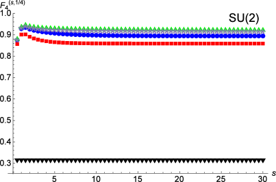
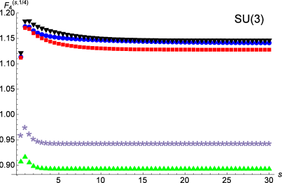
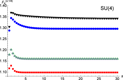
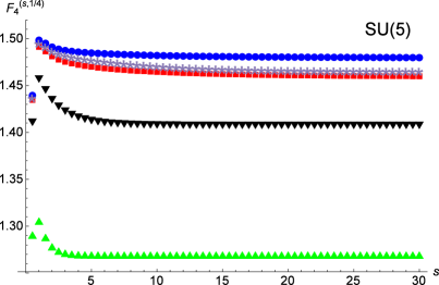
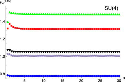
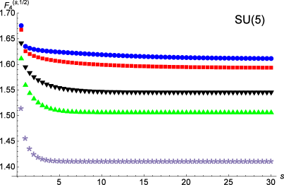
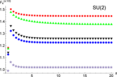
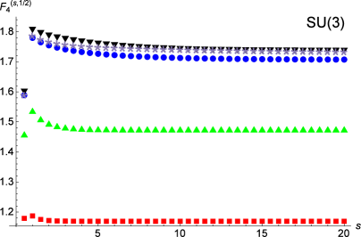
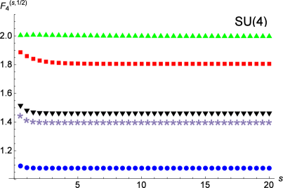
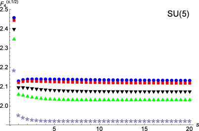
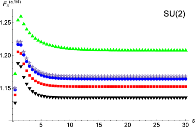
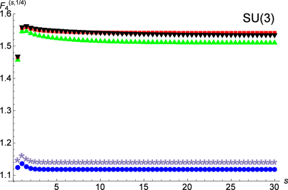
From the above discussion it is clear that we should look at large-$s$ behaviours of the interpolating functions. So let us see $s$-dependences of our interpolating functions. Fig. 1 shows $s$-dependence of the interpolating function $F_{4}^{(s,1/4)}(\tau)$ of the spin-0 leading twist operator for various values of $\tau$ and $N$. We can easily see that the values of the interpolating functions for all the cases become constant for large-$s$ regime. These behaviours are not only for this particular interpolating function but also for all other interpolating functions as long as we use interpolating functions of the type (3.18). See Appendix C for similar results on the other interpolating functions. Furthermore we can analytically show the saturation for large-$s$ in weak coupling regime and at the duality invariant points $\tau=\tau_{S}$ and $\tau=\tau_{TS}$. For details, see Appendix D. Thus we should pick $s$ from the region having the plateau behaviour. These plots indicate that we can regard $s=30$ as sufficiently large $s$.

3.4.3 Choice of $\alpha$

The parameter $\alpha$ determines the type of branch cuts of the interpolating functions. In [38] it was discussed for the standard FPR (3.2) that correct values of $\alpha$ would be related to analytic properties of exact results. For example, if observables under consideration had square type of branch cuts, then interpolating functions with $\alpha=1/2$ would tend to be better approximations. Since we do not know analytic properties of the anomalous dimensions, we do not know what should be the correct value of $\alpha$ from this viewpoint.

However, we now see that the upper bounds obtained by the bootstrap are useful to find “wrong” choices of $\alpha$. In the large-$N$ limit, the upper bounds on the anomalous dimensions are [23, 30]

$$\lim_{N\rightarrow\infty}\gamma_{0,2,4}\leq 2.$$ (3.29)

If a planar limit of an interpolating function breaks this bound considerably, then we can regard this interpolating function as the wrong choice.

Figure 2: The planar limits of the interpolating functions $F_{4}^{(30,1/2)}$ (blue dotted line) and $F_{4}^{(30,1/4)}$ (green dashed line) with the upper bound by the bootstrap in the large-$N$ limit (shaded region). [Left] The spin-0 case. [Right] The spin-2 case.

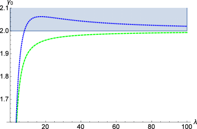
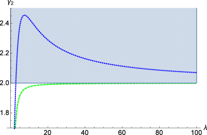
Let us consider the spin-0 and spin-2 cases. For these cases, the maximum of $m$ is $m=4$. By the above arguments in this subsection, we expect that the best approximation among our interpolating function is either $F_{4}^{(s,1/2)}(\tau)$ or $F_{4}^{(s,1/4)}(\tau)$ with sufficiently large $s$. As we discussed, we can regard $s=30$ as sufficiently large $s$. Therefore $F_{4}^{(30,1/2)}(\tau)$ or $F_{4}^{(30,1/4)}(\tau)$ would give the best approximation (Their explicit forms are written in appendix F). In fig. 2 we plot the planar limits of the interpolating functions $F_{4}^{(30,1/2)}(\tau)$ and $F_{4}^{(30,1/4)}(\tau)$, whose expressions are

$$\left.F_{4}^{(30,1/2)}(\tau)\right|_{\rm spin0,planar} = 2\lambda\sqrt{\frac{\lambda+4.14281}{\lambda^{3}+1.8719\lambda^{2}+15.9554\lambda+18.1724}},\mbox{$$}$$

$$\left.F_{4}^{(30,1/4)}(\tau)\right|_{\rm spin0,planar} = \frac{6\lambda}{\left(81\lambda^{4}+109.116\lambda^{3}+473.741\lambda^{2}+1984.4\lambda+1558.55\right)^{1/4}},\mbox{$$}$$

$$\left.F_{4}^{(30,1/2)}(\tau)\right|_{\rm spin2,planar} = 2\lambda\sqrt{\frac{\lambda+7.79869}{\lambda^{3}+0.49032\lambda^{2}+13.8773\lambda+17.7339}},\mbox{$$}$$

$$\left.F_{4}^{(30,1/4)}(\tau)\right|_{\rm spin2,planar} = \frac{50\lambda}{\left(390625\lambda^{4}+108254\lambda^{3}+637497.\lambda^{2}+2643220\lambda+2019870\right)^{1/4}},\mbox{$$}$$

together with the upper bounds (3.29) by the bootstrap. We see that the interpolating functions $F_{4}^{(30,1/2)}(\tau)$ both for spin-0 and spin-2 cases break the upper bounds by the conformal bootstrap considerably while $F_{4}^{(30,1/4)}(\tau)$ does not. This indicates that the interpolating function $F_{4}^{(30,1/2)}(\tau)$ is the wrong choice although its a priori reason is unclear. Thus we expect that $F_{4}^{(30,1/4)}(\tau)$ gives the best approximation and uses the interpolating function $F_{4}^{(30,1/4)}(\tau)$ for comparison with the $\mathcal{N}=4$ superconformal bootstrap. It would be interesting if one can relate this to analytic property of the dimension in the spirit of [38].

4 Results on the leading twist operators for finite $N$

In this section we present our result on the leading twist operators and compare this with the $\mathcal{N}=4$ superconformal bootstrap. We also discuss the image of the conformal manifold in the space of the dimensions. Finally We study the dimension of the sub-leading twist operator and the level crossing phenomenon with the leading twist operator.

4.1 Comparison with the $\mathcal{N}=4$ superconformal bootstrap

In this subsection we compare our interpolating functions with the conjecture [23] by the conformal bootstrap that the upper bounds on the dimensions of the leading twist operators are saturated at one of the duality invariant points $\tau=\tau_{S}=i$ and $\tau=\tau_{TS}=e^{i\pi/3}$.

4.1.1 Spin-0

Figure 3: The interpolating function $F_{4}^{(30,1/4)}(\tau=i/g)$ for the spin-0 operator is plotted against the gauge coupling $g$ for $\theta=0$ (blue dots). The red dashed line denotes the weak coupling expansion up to four loop. The shaded region and horizontal black solid line are the upper bounds and corner values obtained by the $\mathcal{N}=4$ superconformal bootstrap, respectively.

Figure 4: A similar plot as fig. 3 for $\theta=\pi$. The interpolating function $F_{4}^{(30,1/4)}(\tau=1/2+i/g)$ for the spin-0 operator is plotted as a function of $g$ together with the 4-loop result. Note that $g=2/\sqrt{3}$ corresponds to $\tau=\tau_{TS}=e^{i\pi/3}$.

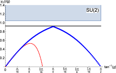
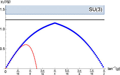
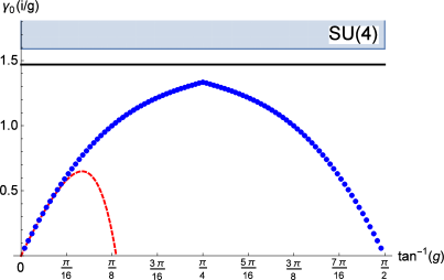
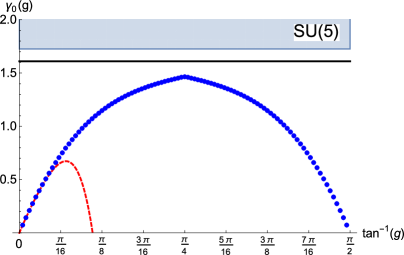
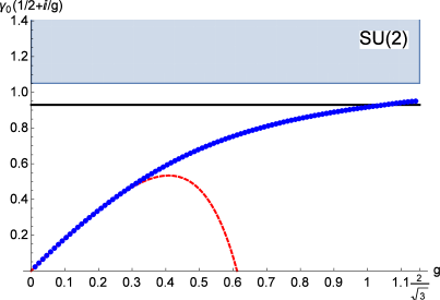
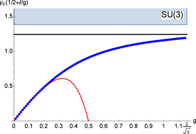
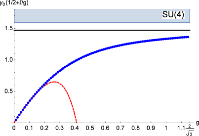
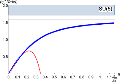
We begin with the spin-0 leading twist operator. By the arguments in sec. 3.4, we expect that the best approximation among our interpolating functions is $F_{4}^{(s,1/4)}(\tau)$ with sufficiently large $s$ and $s=30$ can be regarded as sufficiently large $s$. Therefore we use the interpolating function $F_{4}^{(30,1/4)}(\tau)$ for comparison with the conformal bootstrap, whose explicit forms are written in appendix F. This gives our predictions of the dimension for arbitrary values of the gauge coupling $\tau$ and $N$.

In order to compare our interpolating function with the $\mathcal{N}=4$ superconformal bootstrap, we shall ask where the interpolating function takes its maximal value as a function of $\tau$. We expect that the maximal value is given at either of the duality invariant points $\tau=\tau_{S}$ or $\tau=\tau_{TS}$ if the interpolating function reasonably approximates the dimension. Note that the duality invariant points are also quite special for our interpolating functions. By construction our interpolating functions always have local extremum at $\tau=\tau_{S}$ and $\tau=\tau_{TS}$ because the building block $E_{s}(\tau)$ of the interpolating functions has local minimum at these points for arbitrary $s$. What is nontrivial here is whether one of the extremum of the interpolating function at $\tau=\tau_{S},\tau_{TS}$ is global maximum or not. We will see soon that the global maximum is given by $\tau=\tau_{TS}$.

In fig. 3 we plot coupling dependence of the interpolating function $F_{4}^{(30,1/4)}$ for $\theta=0$. Note that $\tan^{-1}{g}=\pi/4$ corresponds to the duality invariant point $\tau=\tau_{S}=i$ under the $\mathbf{S}$-transformation. First we easily see that the interpolating function is consistent with the upper bounds for all the values of $N$. Next we observe that the interpolating function has the peak at $g=1$, namely, $\tau=\tau_{S}$. This indicates that $\tau=\tau_{S}$ gives the local maximum of the interpolating function. In fig. 4, we give similar plots for $\theta=\pi$ as fig. 3, whose right end $g=2/\sqrt{3}$ corresponds to the duality invariant point $\tau=\tau_{TS}$. We again see that the interpolating functions have the local maximum at $\tau=\tau_{TS}$.

	$SU(2)$	$SU(3)$	$SU(4)$	$SU(5)$	$SU(6)$	$SU(7)$
$\sqrt{a}$	0.86603	1.4142	1.9365	2.4495	2.9580	3.4641
$F_{4}^{(30,1/4)}(\tau_{S})$	0.916879	1.15649	1.33316	1.46501	1.56427	1.63975
$F_{4}^{(30,1/4)}(\tau_{TS})$	0.950352	1.18875	1.36267	1.49133	1.58747	1.66015
Corner value	0.93	1.24	1.47	1.61	1.7	1.78
Strict upper bound	1.05	1.38	1.59	1.726	1.816	1.878

Table 2: The interpolating function for spin-0 at the duality invariant points and data from the $\mathcal{N}=4$ superconformal bootstrap.

Which of the duality invariant points does give the global maximum? In table 2, we explicitly write down the values of the interpolating functions at $\tau=\tau_{S}$ and $\tau=\tau_{TS}$ for various $N$. The table tells us that the interpolating function has the larger values at $\tau=\tau_{TS}$ than the one at $\tau=\tau_{S}$. Actually we have checked that this is true for many other values of $N$. Thus we conclude that the interpolating function has the global maximum at $\tau=\tau_{TS}$.

Figure 5: Comparison of the interpolating function $F_{4}^{(30,1/4)}(\tau)$ at the duality invariant points with the $\mathcal{N}=4$ superconformal bootstrap for the spin-0 case. The horizontal axis denotes the square root of the central charge: $\sqrt{a}$. The black circle symbols are the upper bounds of the anomalous dimension by the $\mathcal{N}=4$ superconformal bootstrap while the red triangles are the corner values. The green dashed and blue solid lines are $F_{4}^{(30,1/4)}(\tau_{S})$ and $F_{4}^{(30,1/4)}(\tau_{TS})$, respectively. The red dashed line shows $2-16/N^{2}$, which is obtained by numerical fitting of the corner values in the large-$a$ regime [23].

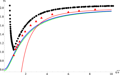
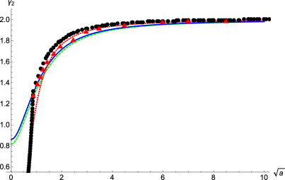
In fig. 5, we plot the values of our interpolating function at the duality invariant points and the data of the $\mathcal{N}=4$ superconformal bootstrap. The horizontal axis is $\sqrt{a}$, where $a$ is the central charge given by

$$a=\frac{N^{2}-1}{4}.$$ (4.1)

Note that information on the gauge group in the $\mathcal{N}=4$ superconformal bootstrap is packaged into the central charge $a$.

As discussed above the interpolating function $F_{4}^{(30,1/4)}(\tau)$ has the greater values at $\tau=\tau_{TS}$ than the one at $\tau=\tau_{S}$. Thus “prediction” for the maximum of the dimension from our interpolating functions is $F_{4}^{(30,1/4)}(\tau_{TS})$, whose formula is explicitly given by

$$F_{4}^{(30,1/4)}(\tau_{TS})=\frac{2N}{\left(N^{4}+1.16663N^{3}+36.3865N^{2}+66.0665N+10.8232\right)^{1/4}}.$$ (4.2)

From fig. 5 we see that our result is close to the corner values in the small-$a$ regime and large-$a$ regime but there are about $10\%$ discrepancies in the intermediate regime. To interpret this, note that the accuracy of the interpolating function should depend on $a$ (or equivalently $N$) for the following two reasons. First of all, we have imposed matching with the holographic computation in the supergravity limit: $\lambda\gg 1,N\gg 1$ and consistency with the upper bound (3.29) in the planar limit. Since the maximal value of the interpolating functions satisfying these conditions is two, our interpolating function matches with the corner values in the large-$a$ regime almost by construction. Second, recalling that the effective coupling constant is $gN$ rather than $g$, we know that the weak coupling expansion is more precise for the small-$a$ regime. Thus the intermediate region is harder to be approximated by our interpolating functions compared to the other regime. Hence, the interpolating function would give relatively worst approximation in the intermediate regime. Thus we interpret the discrepancies as the lack of the accuracy of the interpolating function.

As a result, when we expect good approximations by the interpolating function, we have found that the interpolating function at $\tau=\tau_{TS}$ is very close to the corner values. This supports the conjecture of the $\mathcal{N}=4$ superconformal bootstrap [23] that the upper bounds on the dimensions are saturated at one of the duality-invariant points $\tau=\tau_{S}$ and $\tau=\tau_{TS}$. We certainly expect that if we could include more higher order terms of the perturbation theory, then the interpolating function would have a better approach to the corner values. In the rest of this subsection we will see that similar results hold also for the spin-2 and spin-4 operators.

4.1.2 Spin-2

Figure 6: Similar plots for the spin-2 operator as fig. 3. The interpolating function $F_{4}^{(30,1/4)}(\tau)$ for $\tau=i/g$ is plotted as the function of $g$.

Figure 7: Similar plots for the spin-2 case as fig. 6 for $\theta=\pi$. The interpolating function $F_{4}^{(30,1/4)}(1/2+i/g)$ is plotted as a function of $g$.

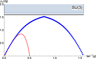
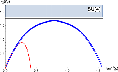
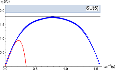
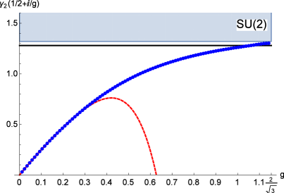
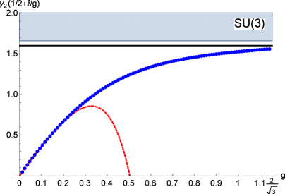
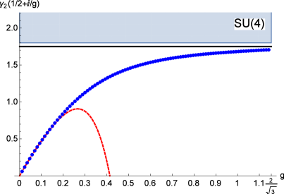
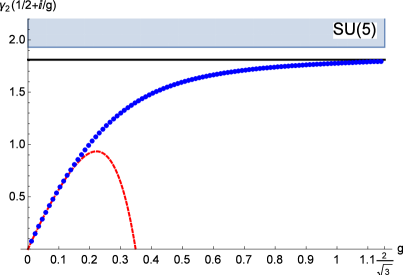
Next we consider the spin-2 leading twist operator. According to sec. 3.4, we expect that the best approximation is given by $F_{4}^{(30,1/4)}(\tau)$ as in the spin-0 case. In fig. 6 and 7, we plot coupling dependence of the interpolating function for $\theta=0$ and $\pi$ as in fig. 3 and 4, respectively. From these figures, we see that $F_{4}^{(30,1/4)}(\tau)$ has the local maximum at the duality invariant points $\tau=\tau_{S}$ and $\tau=\tau_{TS}$. In table 3 we compare $F_{4}^{(30,1/4)}(\tau_{S})$ with $F_{4}^{(30,1/4)}(\tau_{TS})$ as in table 2. This indicates that $F_{4}^{(30,1/4)}(\tau_{TS})$ is always larger than $F_{4}^{(30,1/4)}(\tau_{S})$ and hence we conclude that the interpolating function has the global maximum at $\tau=\tau_{TS}$. For any $N$, the global maximum $F_{4}^{(30,1/4)}(\tau_{TS})$ takes the form

$$F_{4}^{(30,1/4)}(\tau_{TS})=\frac{2N}{\left(N^{4}+0.240002N^{3}+9.224N^{2}+15.5222N+2.90862\right)^{1/4}}.$$ (4.3)

	$SU(2)$	$SU(3)$	$SU(4)$	$SU(5)$	$SU(6)$	$SU(7)$
$\sqrt{a}$	0.86603	1.4142	1.9365	2.4495	2.9580	3.4641
$F_{4}^{(30,1/4)}(\tau_{S})$	1.26131	1.52569	1.68222	1.77664	1.83585	1.87465
$F_{4}^{(30,1/4)}(\tau_{TS})$	1.30315	1.55797	1.70566	1.79367	1.84852	1.88436
Corner value	1.28	1.60	1.75	1.81	1.89	1.92
Strict upper bound	1.32	1.66	1.80	1.93	1.915	1.935

Table 3: The interpolating function for spin-2 at the duality invariant points and data from the $\mathcal{N}=4$ superconformal bootstrap.

In fig. 8, we compare the interpolating function at the duality invariant points with the $\mathcal{N}=4$ superconformal bootstrap. We easily see that the result of $F_{4}^{(30,1/4)}(\tau=\tau_{TS})$ is very close to the corner values in the whole region. This situation is different from the spin-0 case, where we have about $10\%$ discrepancies in the intermediate regime. We interpret this as large-$a$ regime being effectively broader for larger spin case. Indeed $\mathcal{O}(1/N^{2})$ correction to the holographic result for spin-$M$ behaves as $-96/(M+1)(M+6)$ in the supergravity limit [55] and therefore the anomalous dimension with larger-$M$ converges to $\gamma=2$ faster with increasing $N$. Since our interpolating function correctly approximates the large-$a$ regime, we expect that the interpolating function for the spin-2 case gives reliable approximation in broader range of $a$ compared to the spin-0 case. Thus, we expect that our interpolating function provides better approximation in the whole range for the spin-2 case. Since the interpolating function $F_{4}^{(30,1/4)}(\tau_{TS})$ is close to the corner values, our result supports the conjecture in [23] also for the spin-2 case.

Figure 8: A similar plot for the spin-2 operator as in fig. 5. The red dashed line shows $2-4/N^{2}$, which is numerical fitting of the corner values for large-$a$ [23].

4.1.3 Spin-4

Figure 9: Similar plots for the spin-4 operator as fig. 3 and 6. The interpolating function $F_{3}^{(30,1/3)}(\tau)$ for $\theta=0$ is plotted as the function of $g$. The red dashed line denotes the weak coupling expansion up to 3-loop.

Figure 10: A similar plot as fig. 9 for $\theta=\pi$. The interpolating functions $F_{3}^{(30,1/3)}(1/2+i/g)$ for the spin-4 operator is plotted as a function of $g$.

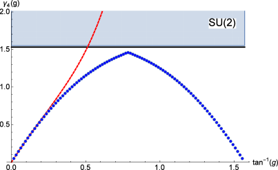
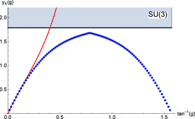
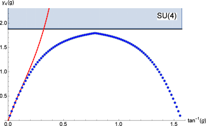
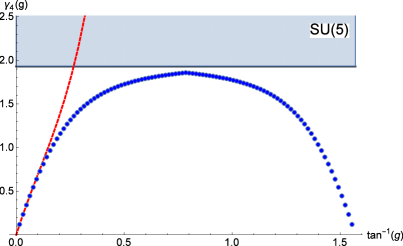
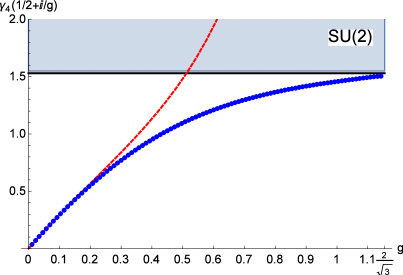
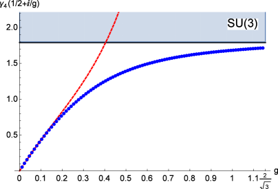
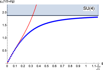
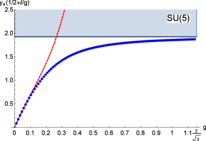
Finally let us consider the spin-4 case. For this case we know the weak coupling expansion only up to three loop. Hence according to sec. 3.4 we shall consider interpolating functions with $m=3$. Contrary to the previous case, now $\alpha$ is uniquely determined as $\alpha=1/3$. Thus we expect that the best approximation is given by the interpolating function $F_{3}^{(30,1/3)}(\tau)$.

	$SU(2)$	$SU(3)$	$SU(4)$	$SU(5)$	$SU(6)$	$SU(7)$
$\sqrt{a}$	0.86603	1.4142	1.9365	2.4495	2.9580	3.4641
$F_{3}^{(30,1/3)}(\tau_{S})$	1.45762	1.68167	1.79528	1.85814	1.8959	1.92016
$F_{3}^{(30,1/3)}(\tau_{TS})$	1.5043	1.7136	1.81717	1.87378	1.90757	1.9292
Corner value	1.53	1.79	1.88	1.93	1.95	1.965
Strict upper bound	1.55	1.80	1.89	1.935	1.955	1.965

Table 4: The interpolating function for spin-4 at the duality invariant points and data from the $\mathcal{N}=4$ superconformal bootstrap.

As in the spin-0 and spin-2 cases, we find from fig. 9 and 10 that the interpolating function $F_{3}^{(30,1/3)}(\tau)$ has local maximum at the duality invariant points $\tau=\tau_{S}$ and $\tau=\tau_{TS}$. From table 4, we see that the interpolating function at $\tau=\tau_{TS}$ is greater than the one at $\tau=\tau_{S}$. Thus our prediction for the maximum anomalous dimension is given by

$$F_{3}^{(30,1/3)}(\tau_{TS})=\frac{2N}{\left(N^{3}+0.136789N^{2}+4.44204N+1.36944\right)^{1/3}}.$$ (4.4)

Fig. 11 compares our result with the $\mathcal{N}=4$ superconformal bootstrap. In this figure we again see the agreement with the corner values in the small-$a$ and large-$a$ regime but there are about $10\%$ discrepancies in the intermediate regime. To interpret this, note that region, where the interpolating function would nicely approximate, is different from the spin-0 and spin-2 cases. First we expect that accuracy of the interpolating function $F_{3}^{(30,1/3)}(\tau)$ is less than the spin-0 and spin-2 cases in the small-$a$ region. This is because the result of the weak coupling expansion is available only up to three loop for this case. Secondly, as discussed in the spin-2 case, large-$a$ regime is effectively broader for the spin-4 case. We expect that the interpolating function is not reliable in the intermediate regime but reliable in the small-$a$ and large-$a$ regime.

Figure 11: A similar plot for the spin-4 case as fig. 5 and 8. The red dashed line shows $2-48/25N^{2}$, which is numerical fitting of the corner values in the large-$a$ regime [23].

As a conclusion of this subsection, we have seen that when we expect reasonable approximation by the interpolating functions, the maximal values of the interpolating functions are close to the corner values of the bootstrap. Thus we conclude that our interpolating function approach strongly supports the conjecture by the $\mathcal{N}=4$ superconformal bootstrap, which states that the upper bounds on the dimensions are saturated at one of the duality-invariant points $\tau=\tau_{S}$ or $\tau=\tau_{TS}$. Obviously, if higher orders of the weak coupling perturbative series become available, then we can obtain more precise interpolating functions. It would be nice if one can obtain the higher order results.

Comments on other gauge groups

A priori our interpolating functions are valid only for the $SU(N)$ gauge group since we have used the weak coupling expansion and holographic computation for the $SU(N)$ case. However, both the data of the bootstrap and the interpolating functions looks continuous for $a\geq 3/4$, whereas the bootstrap data has a cusp at $a=3/4$ ($SU(2)$ case) which is not reproduced by the interpolating functions. Thus we expect that our interpolating functions would reasonably approximate the dimension of the leading twist operator for other gauge groups as long as $a\geq 3/4$. For $a<3/4$, the only possible gauge group is $U(1)$, which is Abelian. The bootstrap results have cusps at $a=3/4$ and this implies a kind of transition from Abelian theory to non-Abelian theory, or from free theory to interacting theory. Contrary to the bootstrap, our interpolating function is smooth across $a=3/4$. Presumably the difference comes from the fact that naive continuation of our interpolating function to general $a$ is a continuation suited to interacting theory and therefore we cannot apply the interpolating function for the $U(1)$ case.

Comments on instanton corrections

The small-$g$ expansions of our interpolating functions contain exponentially suppressed corrections, whose weights are the same as the instanton actions. This feature technically comes from imposing the full $S$-duality. Recently Alday-Korchemsky [43] computed instanton corrections to the dimension of the Konishi operator at $\mathcal{O}(g^{2})$ by expanding around the instanton configuration. They have found that the instanton corrections start from $\mathcal{O}(g^{2})$ and the one-instanton correction for the $SU(2)$ case is given by

$$-\frac{9g^{2}}{20\pi^{2}}\left(e^{2\pi i\tau}+e^{-2\pi i\bar{\tau}}\right).$$ (4.5)

They also computed $n$-instanton correction in the large-$N$ limit as

$$-\frac{27g^{2}}{10\pi^{5/2}n^{3/2}N^{3/2}}\left(e^{2\pi in\tau}+e^{-2\pi in\bar{\tau}}\right)\sum_{d|n}\frac{1}{d^{2}},$$ (4.6)

by using the technique of [70]. On the other hand, the instanton corrections of our interpolating functions with general parameters start from $\mathcal{O}(g^{s+1+{\rm min}(p,q)})$. Since we would like to take $s$ to be sufficiently large as discussed in sec. 3.4.2, the interpolating function $F_{4}^{(s,1/4)}(\tau)$ with large-$s$ cannot reproduce the results (4.5) and (4.6). It is nice if one can construct a new class of interpolating functions, which are consistent with (4.5) and (4.6) in addition to the four-loop result, holographic result and full $S$-duality.

However, it is worthwhile to note that there is a subtlety in [43]. We can also compute instanton corrections to the circular Wilson loop by using the same technique as in [71]. However, the result of [71] states that there are non-trivial instanton corrections to the circular Wilson loop. This does not agrees with the results obtained by summing ladder diagrams [72, 73] and the localization method [74], where instanton corrections are trivial. Thus we should be careful on this point.

Comments on higher order corrections in the planar limit

Although we have used the four-loop result of the weak coupling expansion to construct the spin-0 interpolating functions, there is a seven-loop result in the planar limit [45, 46, 47], whose explicit form is given by (5.2). We did not use the seven-loop result because we also need non-planar corrections to completely fix the coefficients in interpolating functions and the interpolating functions strongly depends on the values of the non-planar higher order corrections for small $N$. Here we just compare the higher order correction in the planar limit with the ones of the interpolating function. The coefficients of the higher order small-$\lambda$ expansion of the interpolating function $F_{4}^{(30,1/4)}(\tau)$ in the planar limit are

$$\left.F_{4}^{(30,1/4)}(\tau)\right|_{{\rm spin-0,planar},\mathcal{O}(\lambda^{5})} = \frac{3(-240\zeta(3)+600\zeta(5)+329)}{64\pi^{5}}\simeq 0.101504,\mbox{$$}$$

$$\left.F_{4}^{(30,1/4)}(\tau)\right|_{{\rm spin-0,planar},\mathcal{O}(\lambda^{6})} = \frac{9(300\zeta(3)-750\zeta(5)-143)}{64\pi^{6}}\simeq-0.0819242,\mbox{$$}$$

$$\left.F_{4}^{(30,1/4)}(\tau)\right|_{{\rm spin-0,planar},\mathcal{O}(\lambda^{7})} = \frac{3\left(360\zeta(3)^{2}-120\zeta(3)(15\zeta(5)+98)+150\zeta(5)(15\zeta(5)+196)+871\right)}{256\pi^{7}}\mbox{$$}$$ (4.7)

$$\simeq 0.0695153,$$

while the correct values are

$$\left.\Delta_{\rm Konishi}\right|_{{\rm planar},\mathcal{O}(\lambda^{5})}\simeq 0.119731,\quad\left.\Delta_{\rm Konishi}\right|_{{\rm planar},\mathcal{O}(\lambda^{6})}\simeq 0.11623,\quad\left.\Delta_{\rm Konishi}\right|_{{\rm planar},\mathcal{O}(\lambda^{7})}\simeq 0.117987.$$ (4.8)

It is attractive if one can construct interpolating functions, which appropriately include the higher order corrections in the planar limit.

Comments on $\alpha^{\prime}$-corrections

Recently the large-$N$ bootstrap for the $\mathcal{N}=4$ SCFT [30] studied structures of $\alpha^{\prime}$-corrections to the dimensions of the leading twist operators in the supergravity limit. It has turned out that the $\alpha^{\prime}$-corrections (large-$\lambda$ expansion) at $\mathcal{O}(1/N^{2})$ starts from $\mathcal{O}(1)$ and the next order is $\mathcal{O}(\alpha^{\prime 3})=\mathcal{O}(\lambda^{-3/2})$. This feature is different from our interpolating functions $F_{4}^{(s,1/4)}(\tau)$ for the spin-0,2 cases and $F_{3}^{(s,1/3)}(\tau)$ for the spin-4 case. Namely their large-$\lambda$ expansions at $\mathcal{O}(1/N^{2})$ start from $\mathcal{O}(1)$ but the next orders are $\mathcal{O}(\lambda^{-1})=\mathcal{O}(\alpha^{\prime 2})$. Furthermore the large-$\lambda$ expansions have only non-negative integer powers of $\lambda^{-1}$. It is illuminating if we can construct interpolating functions to be consistent with the result of [30].

4.2 Image of conformal manifold

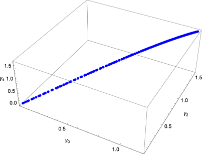
The complex coupling $\tau$ is the exactly marginal parameter and hence the coordinate of the conformal manifold in the $\mathcal{N}=4$ SYM. At every point $\tau$ on the conformal manifold, we have a set of dimensions of the leading twist operators: $(\Delta_{0},\Delta_{2},\Delta_{4},\cdots)$. Since we have constructed the approximations of $(\Delta_{0},\Delta_{2},\Delta_{4})$ by the interpolating functions, we can draw an image of the conformal manifold projected to the $(\Delta_{0},\Delta_{2},\Delta_{4})$-space.

4.2.1 $SU(2)$ case

Figure 12: The figure shows the image of the conformal manifold for $N=2$ in the $(\gamma_{0},\gamma_{2},\gamma_{4})$-space. We use the interpolating function $F_{4}^{(30,1/4)}(\tau)$ for $\gamma_{0},\gamma_{2}$ and $F_{3}^{(30,1/3)}(\tau)$ for $\gamma_{4}$. We have evaluated the interpolating functions for $\theta=\pi n/5$ with $n=0,1,\cdots,5$. [Left-Top] The 3D plot in the $(\gamma_{0},\gamma_{2},\gamma_{4})$-space. [Right-Top] The projection to the $(\gamma_{0},\gamma_{2})$-plane. The red dashed line shows $\gamma_{2}=(25/18)\gamma_{0}$. [Left-Bottom] The projection to the $(\gamma_{0},\gamma_{4})$-plane. The red dashed line shows $\gamma_{4}=(49/30)\gamma_{0}$. [Right-Bottom] The projection to the $(\gamma_{2},\gamma_{4})$-plane. The red dashed line shows $\gamma_{4}=(147/125)\gamma_{2}$.

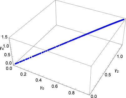
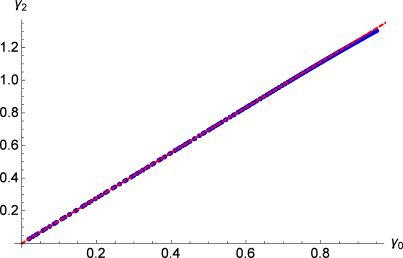
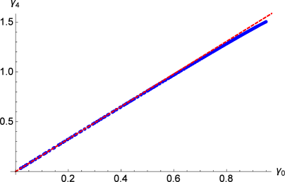
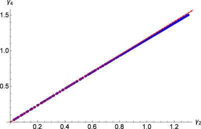
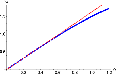
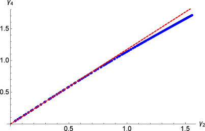
In fig. 12 [Left-Top] we plot the image of the conformal manifold for the $SU(2)$ case projected to the $(\gamma_{0},\gamma_{2},\gamma_{4})$-space. We have sampled the interpolating functions for $\theta=\pi n/5$ with $n=0,1,\cdots,5$ and many values of $g$. The figure shows that the image is almost one continuous straight line and this is different from the following naive expectation. Since we are considering the image of the two dimensional conformal manifold, one naively expects that the image was almost a straight line around the origin but it starts spreading as the dimension increases. This is because the anomalous dimensions in the weak coupling regime are almost independent of $\theta$ but the $\theta$-dependence becomes important in the strongly coupled regime, where the anomalous dimensions become large. Thus, if the above naive expectation was correct, then we should observe six distinguishable lines as we consider the six different values of $\theta$.

Figure 13: Similar plots as fig. 12 for the $SU(3)$ case.

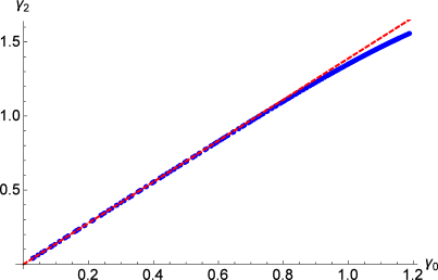
This property has been already observed for the $(\gamma_{0},\gamma_{2})$-plane in [41] by using the different interpolating functions partially invariant under the $SL(2,\mathbb{Z})$ transformations. In [41] the authors found that the slope of the almost straight line in the $(\gamma_{0},\gamma_{2})$-plane is very close to $25/18\simeq 1.38889$, which is the same as the ratio between the one-loop anomalous dimensions:

$$\frac{\left.\gamma_{2}(\tau)\right|_{\mathcal{O}(g)}}{\left.\gamma_{0}(\tau)\right|_{\mathcal{O}(g)}}=\frac{25}{18}.$$ (4.9)

Fig. 12 [Right-Top] shows that this is true also for our interpolating function.

In fig. 12 [Left-Bottom] and 12 [Right-Bottom], we show the similar plots in the $(\gamma_{0},\gamma_{4})$ and $(\gamma_{2},\gamma_{4})$-planes, respectively. The straight lines show $\gamma_{4}=(49/30)\gamma_{0}$ and $\gamma_{4}=(147/125)\gamma_{2}$, whose slopes are the same as

$$\frac{\left.\gamma_{4}(\tau)\right|_{\mathcal{O}(g)}}{\left.\gamma_{0}(\tau)\right|_{\mathcal{O}(g)}}=\frac{49}{30},\quad\frac{\left.\gamma_{4}(\tau)\right|_{\mathcal{O}(g)}}{\left.\gamma_{2}(\tau)\right|_{\mathcal{O}(g)}}=\frac{147}{125}.$$ (4.10)

We find that the images projected to the $(\gamma_{0},\gamma_{4})$ and $(\gamma_{2},\gamma_{4})$-planes are very close to the straight lines as well. This implies that the observation in [41] is also true for the $(\gamma_{0},\gamma_{4})$ and $(\gamma_{2},\gamma_{4})$-planes. In the rest of this subsection we see that the situation is different for the higher $N$ cases.

4.2.2 Higher $N$

Figure 14: Similar plots as fig. 12 and 13 for the $SU(4)$ case.

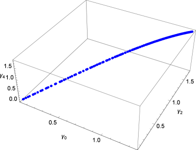
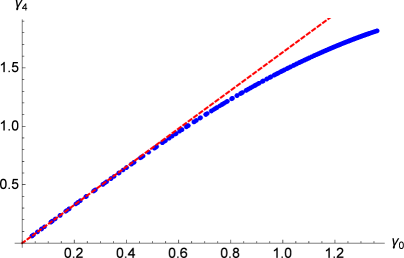
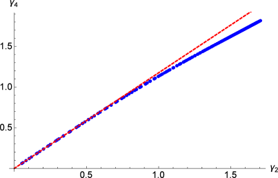
Let us consider the higher $N$ cases. In fig. 13 we give the similar plots as fig. 12 for the $SU(3)$ case. We now find both similarity and dissimilarity from the $SU(2)$ case. The similarity is that the image is still very narrow and therefore looks like one-dimensional. The dissimilarity is that the image is no longer straight line, namely it is curved in the strong coupled regime. To see this in more detail, let us see fig. 13 [Right-Top], which plots the image in the $(\gamma_{0},\gamma_{2})$-plane. The straight line shows again the one-loop relation $\gamma_{2}=(25/18)\gamma_{0}$. The plot tells us that the curve of the image deviates from the straight line when $\gamma_{0}\geq 0.95$. There are two surprising things on this plot. First, the curve is still very narrow after the deviation. Second, the matching with the straight line holds even in the regime, where we cannot naively trust the one-loop approximation for the dimensions. Fig. 13 [Left-Bottom] and 13 [Right-Bottom] imply that similar results hold also on the $(\gamma_{0},\gamma_{4})$ and $(\gamma_{2},\gamma_{4})$-planes, respectively. Fig. 14 shows the similar plots as fig. 12 and 13 for the $SU(4)$ case. We easily see that the result for $N=4$ is qualitatively the same as the $N=3$ case though the deviations from the straight lines are slightly larger. We have checked that similar results hold for other values of $N$.

The above results for $N\geq 3$ are different from those in [41], where the images were still the straight lines even for $N=3$ and $N=4$ while the common feature is that the images are very narrow. As a conclusion, all the interpolating functions constructed so far give very narrow lines for the image of the conformal manifold and we expect that this property is probably true also for the exact results. However, we do not have a definite conclusion on whether the narrow lines are straight or curved though it would be natural to be curved in the strongly coupled regime.

4.3 Level crossing

In this subsection we compare the dimension of the leading twist operator with the one of the subleading leading operator and study level crossing phenomenon between the leading and subleading twist operators. We use the word “level crossing” in the following senses. As we increase the coupling, the dimensions of the leading and subleading operators approach each other and the following two things may occur:

1. Operator mixing between them do not occur by some additional protected symmetries and their dimensions cross over.

2. Operator mixing occurs and the dimensions of new eigenstates repel.

We refer to both of the above as level crossing.

In the $\mathcal{N}=4$ SYM, the operator ${\rm Tr}\phi^{I}D^{M}\phi^{I}$ in (1.1) has the dimension $(2+M)$ at the classical level while this becomes very large for large ’t Hooft coupling in the planar limit. This is because this operator is dual to a massive string state and therefore its dimension behaves as $\sim 1/\sqrt{\alpha^{\prime}}\sim\lambda^{1/4}$ [17]. This implies that the operator (1.1) is no longer the leading twist operator in the large-$\lambda$ regime of the planar limit. Indeed we have a family of double trace operators with the same spins, whose dimensions are protected in the planar limit. The double trace operators consist of protected chiral primary operators and their dimensions are independent of $\lambda$ in the planar limit because of large-$N$ factorization. Thus we expect the level crossing in the first sense between the leading and subleading twist operators in the planar limit.

To interpret this, let us recall the Wigner-von Neumann non-crossing rule known in quantum mechanics, which states that levels of states with the same symmetry cannot cross each other. Since the dilatation operator in the $\mathcal{N}=4$ SYM on $\mathbb{R}^{4}$ corresponds to the Hamiltonian on $\mathbb{R}\times S^{3}$, we expect that the dimensions obey the Wigner-von Neumann non-crossing rule. Recently it was discussed [75] that in the problem of the $\mathcal{N}=4$ SYM , $1/N$ plays roles as “interaction energy” of two level system in quantum mechanics. The actual crossing between the Konishi and double trace operators in the planar limit is consistent with the Wigner-von Neumann non-crossing rule if we have additional symmetry in the planar limit. Most promising candidate for such symmetry is the one associated with the integrability, which is supposed to appear in the planar limit. Since we do not expect such additional symmetry beyond the planar limit, we expect that the level crossing in the first sense does not occur for finite $N$ but the one in the second sense occurs for large but finite $N$.

Here we approach the level crossing problem by using our interpolating function for the spin-0 case. The operator (1.1) for $M=0$ is nothing but the Konishi operator ${\rm Tr}\phi^{I}\phi^{I}$, whose dimension is two at the classical level and $2(4\pi\lambda)^{1/4}+\,(\text{corrections})$ for large-$\lambda$ in the planar limit. Next let us also consider the following operators

$${\rm Tr}{\phi^{I}\phi^{I}}{\rm Tr}{\phi^{J}\phi^{J}},\qquad{\rm Tr}{\phi^{I}\phi^{J}}{\rm Tr}{\phi^{I}\phi^{J}}\qquad{\rm Tr}{\phi^{I}\phi^{I}\phi^{J}\phi^{J}},\qquad{\rm Tr}{\phi^{I}\phi^{J}\phi^{I}\phi^{J}},$$ (4.11)

which have naively the same symmetry as the Konishi operator. Particular linear combinations of these operators are eigenvectors of the dilatation operator, which are dimension $4$ in the weak coupling limit. Therefore the lowest dimension among those is the dimension of the subleading twist operators in the weak coupling regime. The dimensions of the operators (4.11) at one loop is given by [76, 77, 37]

$$\Delta_{\rm sub}(\tau)=4+\frac{Nw(N)}{2\pi}g+\mathcal{O}(g^{2}),$$ (4.12)

where $w(N)$ is roots of the equation

$$w^{4}-25w^{3}+\left(188-\frac{160}{N^{2}}\right)w^{2}-\left(384-\frac{1760}{N^{2}}\right)w-\frac{7680}{N^{2}}=0.$$ (4.13)

The dimension of the subleading twist operator is described by the smallest root $w_{-}(N)$ of this equation, which is always negative.

Now we construct interpolating functions for the subleading twist operator by imposing a match with the weak coupling expansion (4.12) and the $SL(2,\mathbb{Z})$ duality. Since we know the perturbative expansion up to only one-loop, we have only one coefficient to be tuned in the $S$-duality invariant interpolating functions. In this situation, we cannot construct the FPR-like interpolating function (3.12) since we needs $m\geq 2$. Hence we use the Alday-Bissi type interpolating function (3.8) for the dimension of the subleading twist operator. For general $s$, we can easily construct the Alday-Bissi type interpolating function as

$$\Delta_{\rm sub}^{(s)}(\tau)=4+\frac{Nw_{-}}{2\pi}\left(\frac{\zeta(2s)}{E_{s}(\tau)}\right)^{1/s}.$$ (4.14)

Figure 15: Comparison of the dimensions of the leading and subleading twist operators with spin-0 as functions of $g$ for $\theta=0$ and various $N$. The red line indicates the subleading interpolating function and the blue line represents the leading interpolating function. The shaded region and horizontal black solid line are the upper bounds and corner values for the leading twist operator obtained by the $\mathcal{N}=4$ superconformal bootstrap, respectively.

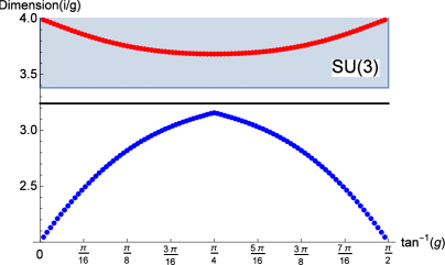
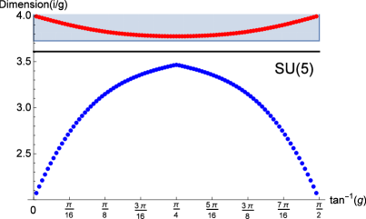
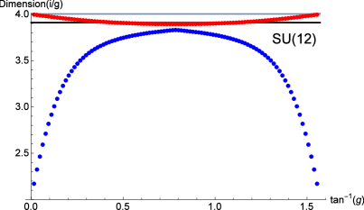
We do have infinitely many $s$-dependent $S$-duality invariant interpolating functions. Which value of $s$ is most appropriate? For this purpose, let us consider the small-$g$ expansion of the interpolating function:

$$\Delta_{\rm sub}^{(s)}(\tau)\simeq 4+\frac{Nw_{-}}{2\pi}g\left(1+\frac{\sqrt{\pi}\Gamma(s-1/2)\zeta(2s-1)}{\Gamma(s)\zeta(2s)}g^{2s-1}\right)^{-1/s},$$ (4.15)

which is true up to non-perturbative corrections. From this expression we can easily see that after the one-loop correction, the next term is a $\mathcal{O}(g^{2s})$ correction and this fact is useful in constraining $s$. First of all, we need $2s\in\mathbb{Z}$ to get integer powers of $g$ in the weak coupling expansion. Next when $s$ is too large, we have large jumps of powers in the weak coupling expansion and therefore want a small value of $s$ as possible. Since the interpolating function is well-defined for $s>1$, we conclude that the most appropriate value of $s$ is $s=3/2$.

Figure 16: Similar plots for $\theta=\pi$ as fig. 15.

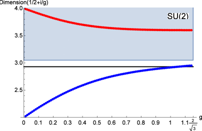
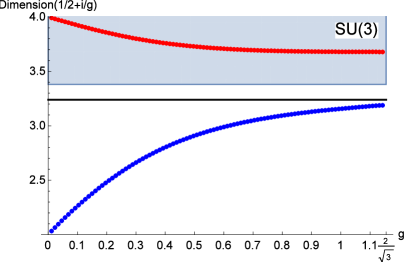
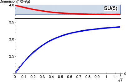
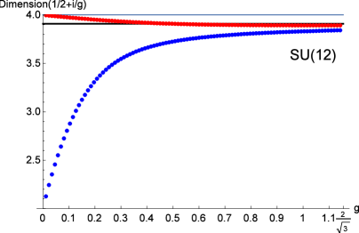
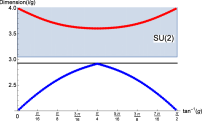
In fig. 15 we compare the interpolating function $\Delta_{\rm sub}^{(3/2)}(\tau)$ for the subleading twist operator with $F_{4}^{(30,1/4)}(\tau)+2$ for the leading twist operator constructed in the last section for $\theta=0$. We easily see from the figure that the interpolating functions do not cross each other for all the values of $N$. We have checked that this is true for other values of $N$, which are not present here. In fig. 16 we give similar plots for $\theta=\pi$ as in fig. 15 in order to test that the above is true also for different values of $\theta$. Again the interpolating functions do not cross each other for all $N$. For $SU(12)$, we observe that the dimension of the leading twist operator becomes very close to the subleading one around $\tau=\tau_{S}$ and $\tau=\tau_{TS}$. Indeed we have found similar results for larger $N$. Thus we conclude that the level crossing in the first sense (actual crossing) does not occur for general finite $N$ but the one in the second sense (small operator mixing) occurs for large but finite $N$.

Interestingly the interpolating function for the subleading twist operator has minimum at the duality invariant points. It would be interesting to find any physical interpretations for that. Finally we have not studied the problem in this subsection for non-zero spin cases. This is because there are no available results for the weak coupling expansions of the subleading twist operators but the one-loop computations for non-zero spins should not be hard. It is nice if one can perform the one-loop computations and the same analysis as in this subsection.

5 Results on Konishi operator in the planar limit

In this section we analyze the dimension of the Konishi operator in the planar limit. While the Konishi operator is the leading twist operator in the weak coupling regime, this has very large dimension in the classical string regime. We approximate the dimension of the Konishi operator in the planar limit in terms of the standard FPR described in sec. 3.1.

5.1 Previous results

First we briefly review previous results on the dimension of the Konishi operator in the planar limit:

$$\lambda=gN=\frac{g_{\rm YM}^{2}N}{4\pi}={\rm fixed},\quad N\rightarrow\infty.$$ (5.1)

In this limit there is a 7-loop computation in the weak coupling expansion [45]:

$$\Delta_{\rm Konishi}(\lambda)\mbox{$$}$$

$$=2+\frac{3\lambda}{\pi}-\frac{3\lambda^{2}}{\pi^{2}}+\frac{21\lambda^{3}}{4\pi^{3}}+\Biggl{[}-39+9\zeta(3)-\frac{45\zeta(5)}{2}\Biggr{]}\frac{\lambda^{4}}{4\pi^{4}}\mbox{$$}$$

$$+\Biggl{[}\frac{945\zeta(7)}{32}-\frac{135\zeta(5)}{16}-\frac{81\zeta(3)^{2}}{16}+\frac{27\zeta(3)}{4}+\frac{237}{16}\Biggr{]}\frac{\lambda^{5}}{\pi^{5}}\mbox{$$}$$

$$+\Biggl{[}-262656\zeta(3)-20736\zeta(3)^{2}+112320\zeta(5)+155520\zeta(3)\zeta(5)\mbox{$$}$$

$$+75600\zeta(7)-489888\zeta(9)-7680\Biggr{]}\frac{\lambda^{6}}{4096\pi^{6}}\mbox{$$}$$

$$+48\Biggl{[}-8784\zeta(3)^{2}+2592\zeta(3)^{3}-4776\zeta(5)-20700\zeta(5)^{2}+24\zeta(3)(357\zeta(5)-1680\zeta(7)+4540)\mbox{$$}$$

$$-26145\zeta(7)-17406\zeta(9)+152460\zeta(11)-44480\Biggr{]}\left(\frac{\lambda}{4\pi}\right)^{7}+\mathcal{O}(\lambda^{8}).$$ (5.2)

There are also some holographic computation of the Konishi operator:

$$\Delta_{\rm Konishi}(\lambda)=2(4\pi\lambda)^{1/4}-2+\frac{2}{(4\pi\lambda)^{1/4}}+\frac{-3\zeta(3)+\frac{1}{2}}{(4\pi\lambda)^{3/4}}.$$ (5.3)

There are some numerical computations using the Thermodynamic Bethe Ansatz (TBA) [78, 79] and we will compare this with our results.

5.2 Comparison with Thermodynamic Bethe Ansatz

Figure 17: [Left] Results on the dimension of Konishi operator in the planar limit. The symbol denotes the numerical result obtained by TBA the lines denote the weak coupling expansion (red dotted), strong coupling expansion (blue dashed), one point Padé approximation $P_{(3|3)}(\lambda)$ (black dot-dashed) and FPR with $(m,n,\alpha)=(15,2,1/28)$ (green solid).
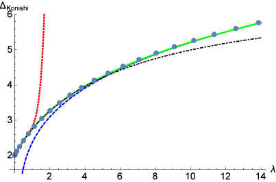
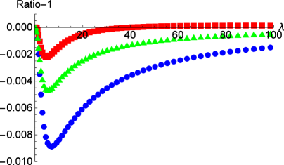
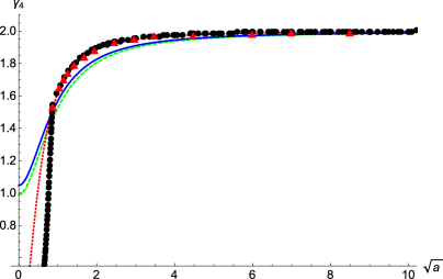
[Right] The relative errors of the interpolating functions from the TBA result. Blue circle, red square and green triangle denote $(m,n,\alpha)=(15,2,1/36)$, $(m,n,\alpha)=(15,2,1/32)$ and $(m,n,\alpha)=(15,2,1/28)$, respectively.

By using the weak and strong coupling expansions, we can construct the interpolating functions. Here we do not use the modular invariant interpolating function (3.11) but use the standard FPR (3.2), which is consistent with the weak coupling expansion (5.2) and the holographic result (5.3) since the dimension of the Konishi operator is not expected to be modular invariant. For this purpose, note that the weak coupling expansion of $\Delta_{\rm Konishi}(\lambda)$ is the power series expansion of $\lambda$ while the holographic result is the one of $\lambda^{-1/4}$. However, if we work with $\Delta_{\rm Konishi}(\lambda)+2$, then the holographic result becomes the power series expansion of $\lambda^{-1/2}$. Thus we consider the FPR-type interpolating functions for $\Delta_{\rm Konishi}(\lambda)+2$ rather than $\Delta_{\rm Konishi}(\lambda)$. More precisely we rewrite the power series expansions of $\Delta_{\rm Konishi}(\lambda)+2$ in terms of $x=\sqrt{\lambda}$ instead of $\lambda$ and consider the interpolating functions $F_{m,n}^{(\alpha)}(x)$ for the expansions. Then the interpolating function approximates the dimension $\Delta_{\rm Konishi}(\lambda)$ by

$$\Delta_{\rm Konishi}(\lambda)\simeq F_{m,n}^{(\alpha)}(x=\sqrt{\lambda})-2.$$ (5.4)

One of subtleties here is that we can construct enormous number of interpolating functions as in the leading twist operators and appropriate choice of $(m,n,\alpha)$ is a priori unclear. However, we have expectations on the appropriate choice at least for $(m,n)$. First for $m$, since the weak coupling expansion in the planar limit is expected to be convergent [80], we expect that interpolating functions with larger $m$ give better approximations. For $n$, we have very few choices, namely $n=0,1,2$. Although the large-$\lambda$ expansion would be asymptotic and its optimized order is unclear, it is natural to expect that the optimized order is larger than $n=2$. Thus we should take $(m,n)$ to be large as possible. It is still unclear what is an appropriate value of $\alpha$. However, this is not so problematic because the interpolating functions with $(m,n)=(15,2)$ are weakly dependent on $\alpha$ as we will see shortly.

In fig. 17 [Left] we compare our result with numerical result obtained by Thermodynamic Bethe Ansatz (TBA) [78]. We also draw the one-point Padé approximant of the weak coupling expansion defined as

$$P_{(m|n)}(\lambda)=\frac{\sum_{k=0}^{m}c_{k}\lambda^{k}}{1+\sum_{k=1}^{n}d_{k}\lambda^{k}},$$ (5.5)

where the coefficients are determined by the correct reproduction of the small-$g$ expansion up to $\mathcal{O}(g^{m+n})$. The one-point Padé approximant in fig. 17 [Left] is the so-called diagonal Padé with $m=n=3$. We easily see that our interpolating function agrees with the TBA result in whole region of $\lambda$. The one-point Padé approximation is good up to around $\lambda=5$ but deviates from the TBA result in stronger coupling region. In fig. 17 [Right] we plot the relative errors of the approximations by the interpolating functions from the TBA result to study precision of their approximations. We find that all the interpolating functions have errors less than $1\%$ in the whole region.

5.3 Analytic property

Figure 18: Analytic property of the FPR with $(m,n,\alpha)=(15,2,1/32)$ as a complex function of $\lambda$. The symbol “$+$” denotes zeros of the rational function $(F_{m,n}^{(\alpha)})^{1/\alpha}$, which give ends of branch cuts of $F_{m,n}^{(\alpha)}$ The green dashed line denotes $|\lambda|=\pi/4$, which is expected radius of convergence in the weak coupling expansion.

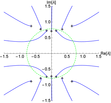
Here we study analytic properties of the interpolating functions following the spirit of [38]. It has been proposed in [38] that when interpolating functions are to give good approximations along an axis in parameter space, then their branch cuts have the following interpretations:

1. The branch cuts are particular to the FPR and the artifact of the approximation by the interpolating function. Namely, this type of branch cut is not helpful in extracting any physical information.

2. The physical quantity, which we try to approximate by the FPR, has an actual branch cut near the branch cut of the FPR. Namely, the branch cut of the FPR approximates the “correct” branch cut of the physical quantity.

3. There is an anti-Stokes line near the branch cut across which perturbation series of the physical quantity changes its dominant part.

Here we expect that some zeros and poles of the interpolating functions approximate analytic properties of the dimension of the Konishi operator.

In fig. 18 we summarize the analytic property of the FPR with $F_{15,2}^{1/32}(x)$ as a complex function of $\lambda$. The symbols denote ends of branch cuts of the interpolating function, which are characterized by zeros and poles of the associated rational function $(F_{m,n}^{(\alpha)})^{1/\alpha}$. The green dashed line denotes $|\lambda|=\pi/4$, which is the expected radius of convergence in the weak coupling expansion from previous works [81, 82, 47]. From this figure, we observe that many ends of branch cuts are located around the circle $|\lambda|=\pi/4$. This is indeed reasonable because one expects that the dimension of Konishi operator has some singularities around radius of convergence of the weak coupling perturbative expansion and so does the interpolating function if the interpolating function approximates the proper analytic properties.

6 Conclusion and discussions

In this paper we have mainly studied the dimensions of the unprotected leading twist operators in the 4d $SU(N)$ $\mathcal{N}=4$ SYM. We have constructed the class of interpolating functions (3.18) to approximate the dimensions. The interpolating functions are consistent with the previous results on the perturbation theory (2.7), holographic computation (2.9) and full S-duality. and give the predictions for arbitrary value of $N$ and the complex gauge coupling $\tau$ in the fundamental region, which particularly includes the duality-invariant points $\tau=i$ and $\tau=e^{i\pi/3}$. We have used our interpolating functions to test the recent conjecture by the $\mathcal{N}=4$ superconformal bootstrap [23], which states that the upper bounds on the dimensions are saturated at either one of the duality-invariant points $\tau=i$ or $\tau=e^{i\pi/3}$. It has turned out that our interpolating functions have the maximum at $\tau=e^{i\pi/3}$. In the regime where we expect reasonable approximations by the interpolating functions, the maximal values are close to the conjectural values in [23]. Thus we conclude that our interpolating function approach strongly supports the conjecture of [23] as well as [41, 37]. In order to construct the interpolating functions we have used the available four-loop or three-loop results of the weak coupling expansions. Obviously, if higher orders of the weak coupling perturbative series become available, then we can obtain more precise interpolating functions which are expected to better approach the corner value at $\tau=e^{i\pi/3}$. It would be nice if one can obtain the higher order results and repeat our analysis in this paper to construct better interpolating functions.

In terms of the interpolating functions, we have drawn the image of the conformal manifold in the space of the dimensions $(\Delta_{0},\Delta_{2},\Delta_{4})$. We have found that the image is almost a line as in [41] despite the conformal manifold being two-dimensional. For the $SU(2)$ case, the line is almost straight, whose slope is the ratio of the one-loop anomalous dimensions as in [41]. For higher $N$, we have seen that the line is curved contrast to [41].

We have also constructed interpolating functions for the subleading twist operator and studied the level crossing phenomenon between the leading and subleading twist operators. We have checked that the interpolating functions for the both operators do not have actual crossing with each other for finite $N$. For large but finite $N$, we have found that the dimension of the leading twist operator becomes very close to the subleading one around $\tau=i$ and $\tau=e^{\pi i/3}$. This implies the small mixing between the two operators. To construct the interpolating function for the sub-leading twist operator, we have used only the one-loop result. Computing two-loop order would give more insights to the level crossing problem. In this paper we have considered only the spin-0 case as there are no one-loop computations for the subleading twist operators with non-zero spins. It would be nice if one can perform the one-loop computations and repeat the same analysis for non-zero spin cases.

We have also studied the dimension of Konishi operator in the planar limit. We have found that our interpolating functions match with the numerical result obtained by Thermodynamic Bethe Ansatz very well. Furthermore we have discussed the analytic property of the relatively best interpolating function in the spirit of [38]. It has turned out that analytic property of the interpolating function reflects the expectations on radius of convergence from the weak coupling perturbation theory.

The key to our interpolating functions is their modular invariance. It would be illuminating if we study other modular invariant observables by our interpolating functions. More challenging direction is to construct interpolating functions for modular forms, which is not modular invariant but have particular transformation properties under $SL(2,\mathbb{Z})$ transformations. It would be also interesting to consider other theories, which enjoy $SL(2,\mathbb{Z})$ duality. Indeed many theories with the $SL(2,\mathbb{Z})$ duality were recently found by torus compactifications of 6d $(1,0)$ theories have the S-duality [83].

Acknowledgements

M. H. thanks Christopher Beem, Leonardo Rastelli and Balt C. van Rees for kindly sending him numerical data in their previous work [23]. We are grateful to Dileep P. Jatkar for helpful comments on the draft. We would like to thank Ofer Aharony, Lorenzo Di Pietro, Mikhail Isachenkov, Dileep P. Jatkar, Zohar Komargodski, Shota Komatsu, Shiraz Minwalla, Ashoke Sen and Tarun Sharma for useful discussions. The work of S. T. was supported by a separate India Israel (ISF/UGC) grant, as well as the Infosys Endowment for the study of the Quantum Structure of Space Time.

Appendix A On numerical computation of non-holomorphic Eisenstein series

In this Appendix we briefly explain how to numerically compute the non-holomorphic Eisenstein series. The non-holomorphic Eisenstein series $E_{s}(\tau)$ has the following expansion (see e.g. sec.5.3 of [84])

$$E_{s}(\tau) = \zeta(2s)({\rm Im}\tau)^{s}+\frac{\sqrt{\pi}\Gamma(s-1/2)}{\Gamma(s)}\zeta(2s-1)({\rm Im}(\tau))^{1-s}\mbox{$$}$$ (A.1)

$$+\frac{4\pi^{s}}{\Gamma(s)}\sqrt{{\rm Im}(\tau)}\sum_{k=1}^{\infty}\sigma_{1-2s}(k)k^{s-\frac{1}{2}}K_{s-\frac{1}{2}}\left(2\pi k{\rm Im}(\tau)\right)\cos{\left(2\pi k{\rm Re}(\tau)\right)},$$

where $\sigma_{s}(k)$ is the divisor function

$$\sigma_{s}(k)=\sum_{d|k}d^{s}.$$ (A.2)

In terms of $(g,\theta)$, this is written as

$$E_{s}(\tau) = \zeta(2s)g^{-s}+\frac{\sqrt{\pi}\Gamma(s-1/2)}{\Gamma(s)}\zeta(2s-1)g^{s-1}\mbox{$$}$$ (A.3)

$$+\frac{4\pi^{s}}{\Gamma(s)}g^{-\frac{1}{2}}\sum_{k=1}^{\infty}\sigma_{1-2s}(k)k^{s-\frac{1}{2}}K_{s-\frac{1}{2}}\left(\frac{2\pi k}{g}\right)\cos{\left(k\theta\right)}.$$

This representation is suitable for numerical computation. When the summation does not converge well, we practically compute the summation at another point connected by the $SL(2,\mathbb{Z})$ symmetry.

Appendix B Another FPR-like modular invariant interpolating function including Alday-Bissi’s one

We can also construct the following interpolating function, which is inspired by the FPR and a generalization of the Alday-Bissi’s interpolating function but a different form:

$$\tilde{F}_{m}^{(s,\alpha)}(\tau)=\Biggl{[}\frac{\sum_{k=1}^{p}c_{k}E_{s+k}(\tau)}{1+\sum_{k=1}^{q}d_{k}E_{s+k}(\tau)}\Biggr{]}^{\alpha}.$$ (B.1)

We determine the coefficients $c_{k}$ and $d_{k}$ such that expansion of $\tilde{F}_{m}^{(s,\alpha)}$ around $g=0$ agrees with the one of $\gamma_{M}(g)$ up to $\mathcal{O}(g^{m+1})$. For $q=0$, this is nothing but the Alday-Bissi’s interpolating function and we consider $q\neq 0$ case below.

Matching at $\mathcal{O}(g)$ leads us to

$$\alpha(-p+q)=1,\quad\left(\frac{c_{s+p}\zeta(2s+2p)}{d_{s+q}\zeta(2s+2q)}\right)^{\alpha}=s_{1}.$$ (B.2)

Imposing matching of other orders leads

$$p+q=m.$$ (B.3)

Therefore we get

$$p=\frac{1}{2}\left(m-\frac{1}{\alpha}\right),\quad q=\frac{1}{2}\left(m+\frac{1}{\alpha}\right).$$ (B.4)

We also require

$$p,q\in\mathbb{Z}_{\geq 1},$$ (B.5)

which implies

$$\alpha=\left\{\begin{matrix}\frac{1}{2\ell+1}&{\rm for}&m:{\rm odd}\cr\frac{1}{2\ell}&{\rm for}&m:{\rm even}\end{matrix}\right.,\quad{\rm with}\ \ell\in\mathbb{Z}.$$ (B.6)

In the main text we do not consider this type of interpolating functions. But it would be interesting to compare the interpolating function with the bootstrap.

Appendix C $s$-dependence of other interpolating functions

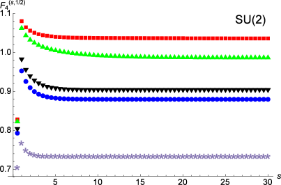
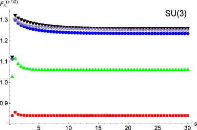
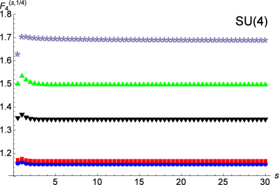
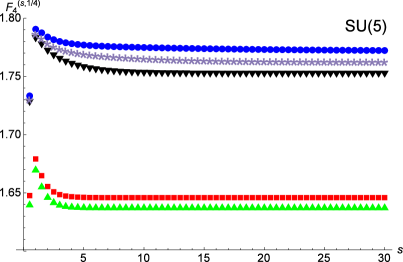
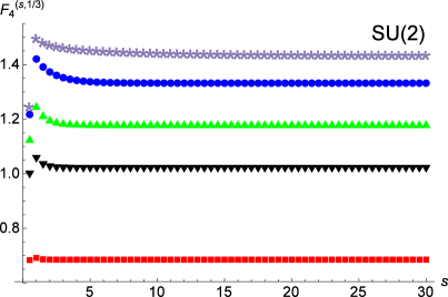
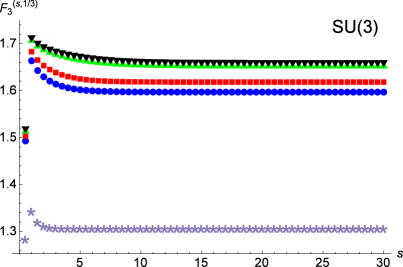
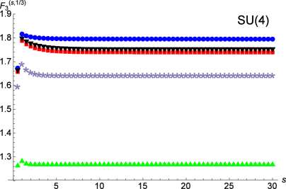
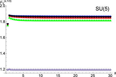
In this appendix we present $s$-dependence of various interpolating functions, in fig. 19,20, 21 and 22. We find that all the results are similar to fig. 1.

Figure 19: $s$-dependence of the interpolating function $F_{4}^{(s,1/2)}(\tau)$ for the spin-0 leading twist operator at randomly chosen five points $\tau=(r_{1},\cdots,r_{5})$. ($r_{1}$: blue circle, $r_{2}$: red square, $r_{3}$: green triangle, $r_{4}$: black inverse triangle, $r_{5}$: purple asterisk) [Left-Top] $SU(2)$ case, $(r_{1},r_{2},r_{3},r_{4},r_{5})$ $\simeq$ $(0.3377+0.4745i,0.8231+0.9956i,0.5698+0.5929i,0.8193+0.7029i,0.7449+0.34278i)$. [Right-Top] $SU(3)$ case, $(r_{1},r_{2},r_{3},r_{4},r_{5})$ $\simeq$ $(0.1185+0.8770i,0.1236+0.3748i,0.09718+0.6059i,0.6656+0.8062i,0.015689+0.9403i)$. [Left-Bottom] $SU(4)$ case, $(r_{1},r_{2},r_{3},r_{4},r_{5})$ $\simeq$ $(0.9907+0.2714i,0.3436+0.3845i,0.2747+0.07620i,0.03894+0.4271i,0.9893+0.4049i)$. [Right-Bottom] $SU(5)$ case. $(r_{1},r_{2},r_{3},r_{4},r_{5})$ $\simeq$ $(0.4757+0.9538i,0.7171+0.8886i,0.3572+0.07676i,0.5935+0.5138i,0.2600+0.4709i)$.

Figure 20: Similar plots as fig. 19 for the interpolating function $F_{4}^{(s,1/2)}(\tau)$ of the spin-2 case. [Left-Top] $(r_{1},r_{2},r_{3},r_{4},r_{5})$ $\simeq$ $(0.3377+0.4745i,0.8231+0.9956i,0.5698+0.5929i,0.8193+0.7029i,0.7449+0.3428i)$. [Right-Top] $(r_{1},r_{2},r_{3},r_{4},r_{5})$ $\simeq$ $(0.1185+0.8770i,0.1236+0.3748i,0.09718+0.6059i,0.6656+0.8062i,0.01569+0.9403i)$. [Left-Bottom] $(r_{1},r_{2},r_{3},r_{4},r_{5})$ $\simeq$ $(0.9907+0.2714i,0.3436+0.3845i,0.2747+0.07620i,0.03894+0.4271i,0.9893+0.4049i)$. [Right-Bottom] $(r_{1},r_{2},r_{3},r_{4},r_{5})$ $\simeq$ $(0.4757+0.9538i,0.7171+0.8886i,0.3572+0.07676i,0.5935+0.5138i,0.2600+0.4709i)$.

Figure 21: Similar plots as fig. 19 and 20 for the interpolating function $F_{4}^{(s,1/4)}(\tau)$ of the spin-2 case. [Left-Top] $(r_{1},r_{2},r_{3},r_{4},r_{5})$ $\simeq$ $(0.3422+0.2076i,0.3290+0.08323i,0.4127+0.5518i,0.2687+0.6024i,0.390+0.3754i)$. [Right-Top] $(r_{1},r_{2},r_{3},r_{4},r_{5})$ $\simeq$ $(0.7971+0.2347i,0.6482+0.9407i,0.2732+0.8653i,0.4621+0.2902i,0.07740+0.4130i)$. [Left-Bottom] $(r_{1},r_{2},r_{3},r_{4},r_{5})$ $\simeq$ $(0.1233+0.2514i,0.1242+0.2581i,0.8283+0.4928i,0.7952+0.1749i,0.4156+0.9410i)$. [Right-Bottom] $(r_{1},r_{2},r_{3},r_{4},r_{5})$ $\simeq$ $(0.5265+0.5726i,0.02538+0.5655i,0.7295+0.3379i,0.3772+0.6248i,0.4563+0.4726i)$.

Figure 22: Similar plots as fig. 19, 20 and 21 for the interpolating function $F_{3}^{(s,1/3)}(\tau)$ of the spin-4 case. [Left-Top] $(r_{1},r_{2},r_{3},r_{4},r_{5})$ $\simeq$ $(0.1569+0.7136i$, $0.001963+0.2593i$, $0.7151+0.3154i$, $0.2043+0.3075i$, $0.2278+0.8969i)$. [Right-Top] $(r_{1},r_{2},r_{3},r_{4},r_{5})$ $\simeq$ $(0.4293+0.1589i$, $0.7140+0.6887i$, $0.6629+0.7537i$, $0.6183+0.7089i$, $0.4724+0.1022i)$. [Left-Bottom] $(r_{1},r_{2},r_{3},r_{4},r_{5})$ $\simeq$ $(0.06265+0.9844i$, $0.6319+0.5036i$, $0.9058+0.2708i$, $0.6299+0.2444i$, $0.2900+0.2536i)$. [Right-Bottom] $(r_{1},r_{2},r_{3},r_{4},r_{5})$ $\simeq$ $(0.4256+0.9369i$, $0.4141+0.6878i$, $0.9963+0.7780i$, $0.7001+0.9990i$, $0.3334+0.02433i)$.

Appendix D Saturation of interpolating function for weak coupling and at duality invariant points for large-$s$

The coefficients in the interpolating function are determined only by the perturbative part of the Eisenstein series:

$$\left.E_{s}(\tau)\right|_{\rm perturbative}=\zeta(2s)g^{-s}+\frac{\sqrt{\pi}\Gamma(s-1/2)}{\Gamma(s)}\zeta(2s-1)g^{s-1}.$$ (D.1)

In particular for large $s$, the coefficients are determined by the first term. Since $\zeta(2s)$ is almost unity for sufficiently large $s$, the interpolating functions for large $s$ is approximately given by

$$F_{m}^{(s,\alpha)}(\tau)\simeq\Biggl{[}\frac{\sum_{k=1}^{p}c_{k}g^{k}+\mathcal{O}(g^{2s+1})}{\sum_{k=1}^{q}d_{k}g^{k}+\mathcal{O}(g^{2s+1})}\Biggr{]}^{\alpha}\,,$$ (D.2)

and the coefficients $c_{k}$ and $d_{k}$ are almost independent of $s$ for very large $s$. Because of this, the interpolating function in weak coupling regime is almost independent of $s$ for large-$s$.

For values of the interpolating functions at the duality invariant points and for large $s$, we can further solidify our independent of $s$ claim. For this purpose, we should know values of $E_{s}(i)$ and $E_{s}(e^{\frac{i\pi}{3}})$ for large $s$. By using $\zeta_{a}(s)\simeq a^{-s}$ with $a\geq 0$ for large $s$, we find

$$E_{s}(i)\simeq 2,\quad E_{s}(e^{\frac{i\pi}{3}})\simeq 3\left(\frac{\sqrt{3}}{2}\right)^{s},\quad{\rm for}\ s\gg 1.$$ (D.3)

Therefore the interpolating functions at the duality invariant points are given by

$$F_{m}^{(s,\alpha)}(i)\simeq\Biggl{[}\frac{\sum_{k=1}^{p}c_{k}}{\sum_{k=1}^{q}d_{k}}\Biggr{]}^{\alpha},\quad F_{m}^{(s,\alpha)}(e^{\frac{i\pi}{3}})\simeq\Biggl{[}\frac{\sum_{k=1}^{p}c_{k}(\sqrt{3}/2)^{k}}{\sum_{k=1}^{q}d_{k}(\sqrt{3}/2)^{k}}\Biggr{]}^{\alpha},\quad{\rm for}\ s\gg 1.$$ (D.4)

Thus the interpolating function at the duality fixed points is independent of $s$ for large-$s$.

Appendix E $S$-duality interpolating functions with $\lambda^{1/4}$ in the classical string limit

In the main text, we have approximated the dimensions of the leading twist operators by the interpolating functions, which are consistent with the weak coupling expansions, holographic results and full $S$-duality. As the holographic results, we have used the results (2.9) for the double trace operators, which are the subleading twist operators in the weak coupling regime. This is because the operator (1.1) is dual to the massive string state and acquires the very large dimension in the classical string regime.

However, one may wonder if one can construct another modular invariant interpolating functions, which have the same weak coupling expansions but different behaviours say as $\sim\lambda^{1/4}$ in the classical string regime. This may not make sense physically since the dimension of (1.1) would not be modular invariant but this may be useful in future for constructing interpolating functions for other modular invariants with different behaviours in the classical string regime. In this appendix, we try to construct a class of modular interpolating functions, with the same weak coupling expansion and $\lambda^{1/4}$ behaviour in the classical string limit.

To be specific, let us consider the Konishi operator. The dimensions of the Konishi operator behaves as (2.7) for weak coupling and as (5.3) for large-$\lambda$ in the planar limit. Now we would like to construct interpolating functions, which are consistent with (2.7), (5.3) and the full $S$-duality. As a conclusion, we failed to construct a single interpolating function satisfying these properties but we find that a linear combination of multiple interpolating functions which are slight modifications of (3.18), satisfies the properties.

First we discuss that the interpolating functions of the type (3.18), which have been used for the leading twist operators in the main text, cannot satisfy the above properties. Indeed we have explicitly checked this for various cases and we can also show this for large-$s$ in the following way. Recall that the coefficients $c_{k}$ and $d_{k}$ in (3.18) are determined in terms of only perturbative part of the Eisenstein series $E_{s}(\tau)$. Although the perturbative part of $E_{s}(\tau)$ has $\mathcal{O}(g^{-s})$ and $\mathcal{O}(g^{s-1})$ parts, only the $\mathcal{O}(g^{-s})$ part is relevant to determine the coefficients for large-$s$. Thus $c_{k}$ and $d_{k}$ are effectively determined by

$$\Biggl{[}\frac{\sum_{k=1}^{p}\zeta(2s+2k)c_{k}g^{-(s+k)}}{\sum_{k=1}^{q}\zeta(2s+2k)d_{k}g^{-(s+k)}}\Biggr{]}^{\alpha}.$$ (E.1)

While $c_{k}$ and $d_{k}$ are nontrivial function of $N$ in general, we know that their planar limits behave as $\mathcal{O}(N^{q-k})$ since the anomalous dimension is $\mathcal{O}(1)$ in the planar limit. Hence in the planar limit, the interpolating function becomes

$$\Biggl{[}\frac{\sum_{k=1}^{p}\bar{c}_{k}\lambda^{-(s+k)}}{\sum_{k=1}^{q}\bar{d}_{k}\lambda^{-(s+k)}}\Biggr{]}^{\alpha},$$ (E.2)

where

$$\bar{c}_{k}=\lim_{N\rightarrow\infty}\zeta(2s+2k)N^{k-q}c_{k},\quad\bar{d}_{k}=\lim_{N\rightarrow\infty}\zeta(2s+2k)N^{k-q}d_{k}.$$ (E.3)

Since this function becomes $\mathcal{O}(1)$ for large-$\lambda$, the interpolating function (3.18) for large-$s$ cannot have the $\lambda^{1/4}$-law in the classical string limit. Thus we shall consider different types of interpolating functions.

Alternatively let us consider the following type of interpolating functions

$$I_{m}^{(s,t,\alpha)}(\tau)=\Biggl{[}\frac{c_{1}E_{s+t+1}(\tau)+\sum_{k=2}^{p}c_{k}E_{s+k}(\tau)}{\sum_{k=1}^{q}d_{k}E_{s+k}(\tau)}\Biggr{]}^{\alpha},$$ (E.4)

where $c_{1}=\mathcal{O}(N^{q-t-1})$ and the only difference from (3.18) is the presence of the new parameter $t$ in the first term of the numerator. Note that $t$ should be integer to get weak coupling expansion with only integer powers of $g$. By a similar argument as above, we find that the planar limit of this interpolating function for large-$s$ is given by

$$\left.I_{m}^{(s,t,\alpha)}(\tau)\right|_{\rm planar}=\Biggl{[}\frac{\bar{c}_{1}\lambda^{-(s+t+1)}+\sum_{k=2}^{p}\bar{c}_{k}\lambda^{-(s+k)}}{\sum_{k=1}^{q}\bar{d}_{k}\lambda^{-(s+k)}}\Biggr{]}^{\alpha}=\Biggl{[}\frac{\bar{c}_{1}\lambda^{-t}+\sum_{k=2}^{p}\bar{c}_{k}\lambda^{-k+1}}{\sum_{k=1}^{q}\bar{d}_{k}\lambda^{-k+1}}\Biggr{]}^{\alpha},$$ (E.5)

where $\bar{c}_{1}=\lim_{N\rightarrow\infty}\zeta(2s+2)N^{t+1-q}c_{1}$, $\bar{c}_{k}=\lim_{N\rightarrow\infty}\zeta(2s+2k)N^{k-q}c_{k}$ and $\bar{d}_{k}=\lim_{N\rightarrow\infty}\zeta(2s+2k)N^{k-q}d_{k}$. When $t$ is negative, the leading order of this function in the large-$\lambda$ expansion is $\mathcal{O}(\lambda^{-\alpha t})$. Thus the interpolating function of the class (E.4) can have the $\lambda^{1/4}$-law in the classical string limit by appropriately choosing $\alpha$ and $t$. Indeed, if the ‘to be matched’ term is $\mathcal{O}(\lambda^{c})$, then we have to solve for $-\alpha t=c$.

However the interpolating function $I_{m}^{(s,t,\alpha)}(\tau)$ with $-\alpha t=1/4$ cannot correctly reproduce the subleading order of (5.3), namely $\mathcal{O}(1)$. The reason is that if we consider $I_{4}^{(s,t,\alpha)}(\tau)$ with large-$s$, then the $\lambda^{1/4}$-law uniquely requires $(\alpha,t)=(1/4,-1)$ and therefore the subleading order is $\mathcal{O}(\lambda^{-3/4})$ rather than $\mathcal{O}(1)$. Thus we cannot single interpolating function consistent with (2.7), (5.3) and the full $S$-duality by the type (E.4). Alternatively we find that the following linear combination of $I_{m}^{(s,t,\alpha)}$ satisfies the desired properties:

$$w_{1}I_{4}^{(s,-1,1/4)}(\tau)+w_{2}I_{4}^{(s,0,\alpha)}(\tau)+w_{3}I_{4}^{(s,-1,-1/4)}(\tau),\quad{\rm with}\ w_{1}+w_{2}+w_{3}=1.$$ (E.6)

where all the coefficients including $w_{1},\,w_{2}$ and $w_{3}$ are fixed with $I_{4}^{(s,-1,1/4)}(\tau)$, $I_{4}^{(s,0,\alpha)}(\tau)$ and $I_{4}^{(s,-1,-1/4)}(\tau)$ respectively matching to the $\mathcal{O}(\lambda^{1/4})$, $\mathcal{O}(1)$ and $\mathcal{O}(\lambda^{-1/4})$ coefficients. We could also work with variations of the above scheme with more terms from the large-$\lambda$ expansion in the planar limit and weak coupling expansion though we do not explicitly write their constructions.

Appendix F Explicit forms of interpolating functions

In this appendix we present explicit forms of the interpolating functions used in the main text. It should also be noted that we have to solve linear equations to solve for the unknown coefficients and thus it does not involve numerical approximation. Although we often write their coefficients with 6 digits of precision to avoid too long expressions, we practically use analytic expressions or infinite digits in Mathematica files.

F.1 Leading twist operators

F.1.1 Spin-0

$$F_{4}^{(30,1/2)}(\tau) = \left(0.911891N^{2}E_{32}-0.00719662N\left(-30.5858N^{2}-283.977\right)E_{31}\right)^{1/2}\mbox{$$}$$

$$\Bigl{(}E_{34}+N\left(0.0550286N^{2}+1.39138\right)E_{31}-0.000418683E_{32}\left(-246.029N^{2}-3407.72\right)\mbox{$$}$$

$$-\frac{0.00263066\left(-333.757N^{2}-851.93\right)}{N}E_{33}\Bigr{)}^{-1/2},\mbox{$$}$$

$$F_{4}^{(30,1/4)}(\tau) = 0.95493N\left(E_{31}\right)^{1/4}\Bigl{(}0.303964N^{2}E_{33}-0.0161258N\left(-4.34157N^{2}-186.647\right)E_{32}\mbox{$$}$$ (F.1)

$$+\left(0.0519715N^{4}+1.66309N^{2}\right)E_{31}+1.27324NE_{34}+E_{35}\Bigr{)}^{-1/4}.$$

F.1.2 Spin-2

$$F_{4}^{(30,1/2)}(\tau) = N^{1/2}\left(E_{31}\left(0.225557N^{2}+3.60609\right)+1.75905NE_{32}\right)^{1/2}\mbox{$$}$$

$$\Bigl{(}E_{34}+0.0563893N^{3}E_{31}+0.0276488N^{2}E_{32}+1.12708NE_{31}\mbox{$$}$$

$$+0.78253NE_{33}+\frac{2.05002}{N}E_{33}+1.34134E_{32}\Bigr{)}^{-1/2},\mbox{$$}$$

$$F_{4}^{(30,1/4)}(\tau) = 1.32629N\left(E_{31}\right)^{1/4}\mbox{$$}$$ (F.2)

$$\Bigl{(}0.315612N^{2}E_{33}-6.221361\times 10^{-6}N\left(-8614.58N^{2}-399396\right)E_{32}\mbox{$$}$$

$$+N^{2}\left(0.193391N^{2}+1.54713\right)E_{31}+1.30861NE_{34}+E_{35}\Bigr{)}^{-1/4}.$$

F.1.3 Spin-4

$$F_{3}^{(30,1/3)}(\tau) = 1.55972N(E_{31})^{1/3}\Bigl{(}N\left(0.474295N^{2}+1.36597\right)E_{31}\mbox{$$}$$ (F.3)

$$+0.0749153N^{2}E_{32}+0.987822NE_{33}+E_{34}\Bigr{)}^{-1/3}.$$

F.2 Konishi operator in the planar limit

$$F_{15,2}^{(1/28)} = \frac{4}{(-0.798124x^{2}-0.940303x+1)^{1/28}}\Bigl{(}-0.147129x^{16}-1.33546x^{15}-5.10135x^{14}\mbox{$$}$$

$$-7.68337x^{13}-8.77477x^{12}-19.9647x^{11}-4.97804x^{10}-30.8794x^{9}+7.2648x^{8}-30.131x^{7}\mbox{$$}$$

$$+16.5478x^{6}-18.2566x^{5}+14.0806x^{4}-6.28546x^{3}+5.88638x^{2}-0.940303x+1\Bigr{)}^{1/28},\mbox{$$}$$

$$F_{15,2}^{(1/32)} = \frac{4}{(0.280107x+1)^{1/32}}\Bigl{(}1+0.0405549x^{17}+0.510874x^{16}+2.74729x^{15}+9.80801x^{14}\mbox{$$}$$

$$+8.27997x^{13}+29.56x^{12}+15.0662x^{11}+53.7874x^{10}+17.9808x^{9}+64.1926x^{8}+14.2419x^{7}\mbox{$$}$$

$$+50.8445x^{6}+7.2371x^{5}+25.8369x^{4}+2.13986x^{3}+7.63944x^{2}+0.280107x\Bigr{)}^{1/32},\mbox{$$}$$

$$F_{15,2}^{(1/36)} = 4\times\Bigl{(}0.113713x^{18}+1.1548x^{17}+5.19491x^{16}+39.7286x^{14}+83.2077x^{12}\mbox{$$}$$ (F.4)

$$+117.012x^{10}+113.748x^{8}+75.8133x^{6}+33.17x^{4}+8.59437x^{2}+1\Bigr{)}^{1/36}.$$

References

- [1] L. Avdeev, O. Tarasov, and A. Vladimirov, Vanishing of the three-loop charge renormalization function in a supersymmetric gauge theory, Phys.Lett. B96 (1980) 94–96.
- [2] M. T. Grisaru, M. Rocek, and W. Siegel, Zero Three Loop beta Function in N=4 Superyang-Mills Theory, Phys.Rev.Lett. 45 (1980) 1063–1066.
- [3] W. E. Caswell and D. Zanon, Zero Three Loop Beta Function in the Supersymmetric Yang-Mills Theory, Nucl.Phys. B182 (1981) 125.
- [4] M. F. Sohnius and P. C. West, Conformal Invariance in N=4 Supersymmetric Yang-Mills Theory, Phys.Lett. B100 (1981) 245.
- [5] P. S. Howe, K. Stelle, and P. Townsend, Miraculous Ultraviolet Cancellations in Supersymmetry Made Manifest, Nucl.Phys. B236 (1984) 125.
- [6] S. Mandelstam, Light Cone Superspace and the Ultraviolet Finiteness of the N=4 Model, Nucl.Phys. B213 (1983) 149–168.
- [7] L. Brink, O. Lindgren, and B. E. Nilsson, The Ultraviolet Finiteness of the N=4 Yang-Mills Theory, Phys.Lett. B123 (1983) 323.
- [8] P. Goddard, J. Nuyts, and D. I. Olive, Gauge Theories and Magnetic Charge, Nucl. Phys. B125 (1977) 1.
- [9] C. Montonen and D. I. Olive, Magnetic Monopoles as Gauge Particles?, Phys. Lett. B72 (1977) 117.
- [10] H. Osborn, Topological Charges for N=4 Supersymmetric Gauge Theories and Monopoles of Spin 1, Phys. Lett. B83 (1979) 321.
- [11] A. Sen, Dyon - monopole bound states, selfdual harmonic forms on the multi - monopole moduli space, and SL(2,Z) invariance in string theory, Phys. Lett. B329 (1994) 217–221, [hep-th/9402032].
- [12] C. Vafa and E. Witten, A Strong coupling test of S duality, Nucl. Phys. B431 (1994) 3–77, [hep-th/9408074].
- [13] N. Beisert and M. Staudacher, The N=4 SYM integrable super spin chain, Nucl. Phys. B670 (2003) 439–463, [hep-th/0307042].
- [14] N. Beisert et al., Review of AdS/CFT Integrability: An Overview, Lett. Math. Phys. 99 (2012) 3–32, [arXiv:1012.3982].
- [15] J. M. Drummond, J. Henn, V. A. Smirnov, and E. Sokatchev, Magic identities for conformal four-point integrals, JHEP 01 (2007) 064, [hep-th/0607160].
- [16] J. M. Maldacena, The Large N limit of superconformal field theories and supergravity, Int. J. Theor. Phys. 38 (1999) 1113–1133, [hep-th/9711200]. [Adv. Theor. Math. Phys.2,231(1998)].
- [17] S. S. Gubser, I. R. Klebanov, and A. M. Polyakov, Gauge theory correlators from noncritical string theory, Phys. Lett. B428 (1998) 105–114, [hep-th/9802109].
- [18] E. Witten, Anti-de Sitter space and holography, Adv. Theor. Math. Phys. 2 (1998) 253–291, [hep-th/9802150].
- [19] R. Rattazzi, V. S. Rychkov, E. Tonni, and A. Vichi, Bounding scalar operator dimensions in 4D CFT, JHEP 12 (2008) 031, [arXiv:0807.0004].
- [20] V. S. Rychkov and A. Vichi, Universal Constraints on Conformal Operator Dimensions, Phys. Rev. D80 (2009) 045006, [arXiv:0905.2211].
- [21] S. El-Showk, M. F. Paulos, D. Poland, S. Rychkov, D. Simmons-Duffin, and A. Vichi, Solving the 3D Ising Model with the Conformal Bootstrap, Phys. Rev. D86 (2012) 025022, [arXiv:1203.6064].
- [22] S. El-Showk and M. F. Paulos, Bootstrapping Conformal Field Theories with the Extremal Functional Method, Phys. Rev. Lett. 111 (2013), no. 24 241601, [arXiv:1211.2810].
- [23] C. Beem, L. Rastelli, and B. C. van Rees, The Superconformal Bootstrap, Phys.Rev.Lett. 111 (2013) 071601, [arXiv:1304.1803].
- [24] M. Honda, G. Ishiki, S.-W. Kim, J. Nishimura, and A. Tsuchiya, Supersymmetry non-renormalization theorem from a computer and the AdS/CFT correspondence, PoS LATTICE2010 (2010) 253, [arXiv:1011.3904].
- [25] M. Honda, G. Ishiki, J. Nishimura, and A. Tsuchiya, Testing the AdS/CFT correspondence by Monte Carlo calculation of BPS and non-BPS Wilson loops in 4d N=4 super-Yang-Mills theory, PoS LATTICE2011 (2011) 244, [arXiv:1112.4274].
- [26] S. Catterall, P. H. Damgaard, T. Degrand, R. Galvez, and D. Mehta, Phase Structure of Lattice N=4 Super Yang-Mills, JHEP 11 (2012) 072, [arXiv:1209.5285].
- [27] M. Honda, G. Ishiki, S.-W. Kim, J. Nishimura, and A. Tsuchiya, Direct test of the AdS/CFT correspondence by Monte Carlo studies of N=4 super Yang-Mills theory, JHEP 11 (2013) 200, [arXiv:1308.3525].
- [28] L. F. Alday and A. Bissi, The superconformal bootstrap for structure constants, JHEP 09 (2014) 144, [arXiv:1310.3757].
- [29] L. F. Alday and A. Bissi, Generalized bootstrap equations for SCFT, JHEP 02 (2015) 101, [arXiv:1404.5864].
- [30] L. F. Alday, A. Bissi, and T. Lukowski, Lessons from crossing symmetry at large N, JHEP 06 (2015) 074, [arXiv:1410.4717].
- [31] L. F. Alday and A. Bissi, Unitarity and positivity constraints for CFT at large central charge, arXiv:1606.09593.
- [32] A. Sen, S-duality Improved Superstring Perturbation Theory, JHEP 1311 (2013) 029, [arXiv:1304.0458].
- [33] M. Honda, On Perturbation theory improved by Strong coupling expansion, JHEP 1412 (2014) 019, [arXiv:1408.2960].
- [34] V. Asnin, D. Gorbonos, S. Hadar, B. Kol, M. Levi, and U. Miyamoto, High and Low Dimensions in The Black Hole Negative Mode, Class.Quant.Grav. 24 (2007) 5527–5540, [arXiv:0706.1555].
- [35] T. Banks and T. Torres, Two Point Pade Approximants and Duality, arXiv:1307.3689.
- [36] R. Pius and A. Sen, S-duality improved perturbation theory in compactified type I/heterotic string theory, JHEP 1406 (2014) 068, [arXiv:1310.4593].
- [37] L. F. Alday and A. Bissi, Modular interpolating functions for N=4 SYM, JHEP 1407 (2014) 007, [arXiv:1311.3215].
- [38] M. Honda and D. P. Jatkar, Interpolating function and Stokes Phenomena, Nucl. Phys. B900 (2015) 533–559, [arXiv:1504.02276].
- [39] H. Kleinert and V. Schulte-Frohlinde, Critical properties of phi**4-theories, River Edge, USA: World Scientific (2001).
- [40] V. I. Yukalov and S. Gluzman, Self-similar interpolation in high-energy physics, Phys. Rev. D91 (2015) 125023, [arXiv:1506.09022].
- [41] C. Beem, L. Rastelli, A. Sen, and B. C. van Rees, Resummation and S-duality in N=4 SYM, JHEP 04 (2014) 122, [arXiv:1306.3228].
- [42] M. Bianchi, S. Kovacs, G. Rossi, and Y. S. Stanev, Properties of the Konishi multiplet in N=4 SYM theory, JHEP 0105 (2001) 042, [hep-th/0104016].
- [43] L. F. Alday and G. P. Korchemsky, Revisiting instanton corrections to the Konishi multiplet, arXiv:1605.06346.
- [44] B. Eden, P. Heslop, G. P. Korchemsky, V. A. Smirnov, and E. Sokatchev, Five-loop Konishi in N=4 SYM, Nucl. Phys. B862 (2012) 123–166, [arXiv:1202.5733].
- [45] Z. Bajnok and R. A. Janik, Six and seven loop Konishi from Luscher corrections, JHEP 11 (2012) 002, [arXiv:1209.0791].
- [46] N. Gromov, F. Levkovich-Maslyuk, G. Sizov, and S. Valatka, Quantum spectral curve at work: from small spin to strong coupling in = 4 SYM, JHEP 07 (2014) 156, [arXiv:1402.0871].
- [47] C. Marboe and D. Volin, Quantum spectral curve as a tool for a perturbative quantum field theory, Nucl. Phys. B899 (2015) 810–847, [arXiv:1411.4758].
- [48] A. Kotikov, L. Lipatov, A. Onishchenko, and V. Velizhanin, Three loop universal anomalous dimension of the Wilson operators in N=4 SUSY Yang-Mills model, Phys.Lett. B595 (2004) 521–529, [hep-th/0404092].
- [49] A. Kotikov, L. Lipatov, A. Rej, M. Staudacher, and V. Velizhanin, Dressing and wrapping, J.Stat.Mech. 0710 (2007) P10003, [arXiv:0704.3586].
- [50] F. Fiamberti, A. Santambrogio, C. Sieg, and D. Zanon, Wrapping at four loops in N=4 SYM, Phys.Lett. B666 (2008) 100–105, [arXiv:0712.3522].
- [51] F. Fiamberti, A. Santambrogio, C. Sieg, and D. Zanon, Anomalous dimension with wrapping at four loops in N=4 SYM, Nucl.Phys. B805 (2008) 231–266, [arXiv:0806.2095].
- [52] Z. Bajnok, R. A. Janik, and T. Lukowski, Four loop twist two, BFKL, wrapping and strings, Nucl.Phys. B816 (2009) 376–398, [arXiv:0811.4448].
- [53] V. Velizhanin, The four-loop anomalous dimension of the Konishi operator in N=4 supersymmetric Yang-Mills theory, JETP Lett. 89 (2009) 6–9, [arXiv:0808.3832].
- [54] V. Velizhanin, The Non-planar contribution to the four-loop universal anomalous dimension in N=4 Supersymmetric Yang-Mills theory, JETP Lett. 89 (2009) 593–596, [arXiv:0902.4646].
- [55] F. Dolan and H. Osborn, Superconformal symmetry, correlation functions and the operator product expansion, Nucl.Phys. B629 (2002) 3–73, [hep-th/0112251].
- [56] E. D’Hoker, S. D. Mathur, A. Matusis, and L. Rastelli, The Operator product expansion of N=4 SYM and the 4 point functions of supergravity, Nucl.Phys. B589 (2000) 38–74, [hep-th/9911222].
- [57] G. Arutyunov, S. Frolov, and A. C. Petkou, Operator product expansion of the lowest weight CPOs in N=4 SYM(4) at strong coupling, Nucl.Phys. B586 (2000) 547–588, [hep-th/0005182].
- [58] B. Eden, A. C. Petkou, C. Schubert, and E. Sokatchev, Partial nonrenormalization of the stress tensor four point function in N=4 SYM and AdS / CFT, Nucl. Phys. B607 (2001) 191–212, [hep-th/0009106].
- [59] G. Arutyunov, B. Eden, A. C. Petkou, and E. Sokatchev, Exceptional nonrenormalization properties and OPE analysis of chiral four point functions in N=4 SYM(4), Nucl. Phys. B620 (2002) 380–404, [hep-th/0103230].
- [60] B. Eden and E. Sokatchev, On the OPE of 1/2 BPS short operators in N=4 SCFT(4), Nucl. Phys. B618 (2001) 259–276, [hep-th/0106249].
- [61] L.-S. Tseng, SL(2,Z) multiplets in N=4 SYM theory, JHEP 01 (2003) 071, [hep-th/0212172].
- [62] M. A. Samuel, J. R. Ellis, and M. Karliner, Comparison of the Pade approximation method to perturbative QCD calculations, Phys. Rev. Lett. 74 (1995) 4380–4383, [hep-ph/9503411].
- [63] P. Argyres and M. Unsal, A semiclassical realization of infrared renormalons, Phys.Rev.Lett. 109 (2012) 121601, [arXiv:1204.1661].
- [64] P. C. Argyres and M. Unsal, The semi-classical expansion and resurgence in gauge theories: new perturbative, instanton, bion, and renormalon effects, JHEP 1208 (2012) 063, [arXiv:1206.1890].
- [65] J. G. Russo, A Note on perturbation series in supersymmetric gauge theories, JHEP 1206 (2012) 038, [arXiv:1203.5061].
- [66] I. Aniceto, J. G. Russo, and R. Schiappa, Resurgent Analysis of Localizable Observables in Supersymmetric Gauge Theories, arXiv:1410.5834.
- [67] M. Honda, Borel Summability of Perturbative Series in 4D and 5D =1 Supersymmetric Theories, Phys. Rev. Lett. 116 (2016), no. 21 211601, [arXiv:1603.06207].
- [68] T. Azeyanagi, M. Fujita, and M. Hanada, From the planar limit to M-theory, Phys. Rev. Lett. 110 (2013), no. 12 121601, [arXiv:1210.3601].
- [69] T. Azeyanagi, M. Hanada, M. Honda, Y. Matsuo, and S. Shiba, A new look at instantons and large-N limit, JHEP 05 (2014) 008, [arXiv:1307.0809].
- [70] N. Dorey, T. J. Hollowood, V. V. Khoze, M. P. Mattis, and S. Vandoren, Multi-instanton calculus and the AdS / CFT correspondence in N=4 superconformal field theory, Nucl. Phys. B552 (1999) 88–168, [hep-th/9901128].
- [71] M. Bianchi, M. B. Green, and S. Kovacs, Instanton corrections to circular Wilson loops in N=4 supersymmetric Yang-Mills, JHEP 04 (2002) 040, [hep-th/0202003].
- [72] J. K. Erickson, G. W. Semenoff, and K. Zarembo, Wilson loops in N = 4 supersymmetric Yang-Mills theory, Nucl. Phys. B582 (2000) 155–175, [hep-th/0003055].
- [73] N. Drukker and D. J. Gross, An Exact prediction of N=4 SUSYM theory for string theory, J. Math. Phys. 42 (2001) 2896–2914, [hep-th/0010274].
- [74] V. Pestun, Localization of gauge theory on a four-sphere and supersymmetric Wilson loops, Commun.Math.Phys. 313 (2012) 71–129, [arXiv:0712.2824].
- [75] G. P. Korchemsky, On level crossing in conformal field theories, JHEP 03 (2016) 212, [arXiv:1512.05362].
- [76] G. Arutyunov, S. Penati, A. C. Petkou, A. Santambrogio, and E. Sokatchev, Nonprotected operators in N=4 SYM and multiparticle states of AdS(5) SUGRA, Nucl. Phys. B643 (2002) 49–78, [hep-th/0206020].
- [77] N. Beisert, C. Kristjansen, and M. Staudacher, The Dilatation operator of conformal N=4 superYang-Mills theory, Nucl. Phys. B664 (2003) 131–184, [hep-th/0303060].
- [78] N. Gromov, V. Kazakov, and P. Vieira, Exact Spectrum of Planar Supersymmetric Yang-Mills Theory: Konishi Dimension at Any Coupling, Phys. Rev. Lett. 104 (2010) 211601, [arXiv:0906.4240].
- [79] S. Frolov, Konishi operator at intermediate coupling, J. Phys. A44 (2011) 065401, [arXiv:1006.5032].
- [80] G. ’t Hooft, On the Convergence of Planar Diagram Expansions, Commun. Math. Phys. 86 (1982) 449.
- [81] N. Beisert, B. Eden, and M. Staudacher, Transcendentality and Crossing, J. Stat. Mech. 0701 (2007) P01021, [hep-th/0610251].
- [82] D. Volin, The 2-Loop generalized scaling function from the BES/FRS equation, arXiv:0812.4407.
- [83] M. Del Zotto, C. Vafa, and D. Xie, Geometric engineering, mirror symmetry and , JHEP 11 (2015) 123, [arXiv:1504.08348].
- [84] O. Klevang, Automorphic Forms in String Theory, .