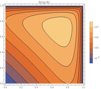
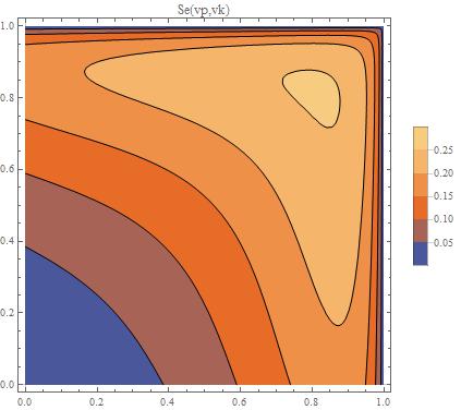
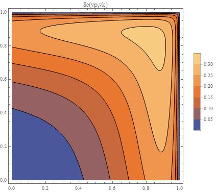
Momentum correlations of scattered particles in quantum field theory: one-loop entanglement generation

Ricardo Faleiro ricardoandremiguel@hotmail.com Rafael Pavão Helder Alexander Brigitte Hiller Alex Blin Marcos Sampaio CFisUC – Department of Physics
University of Coimbra, 3004 -516 Coimbra, Portugal
Universidade Federal de Minas Gerais – Departamento de Física – ICEx
P.O. BOX 702, 30.161-970, Belo Horizonte MG – Brazil
Abstract

We compute the entanglement entropy variation between initial (separable or entangled in the momenta) and final states ΔSEΔsubscript𝑆𝐸\Delta S_{E} in an elastic scattering of a bipartite system composed by two interacting scalar particles. We perform a quantum field theoretical calculation to one loop order and verify that ΔSEΔsubscript𝑆𝐸\Delta S_{E} changes as we vary the energy of incoming particles and the coupling strength in a non-trivial way.

keywords:
Entanglement , Scattering ,
journal: Journal of  Templates

1 Introduction

Relativistic aspects of quantum entanglement have challenged physicists for more than eighty years now, the milestone being the famous Einstein-Podoslky-Rosen (EPR) gedankenexperiment [1]. They concluded that either single particle entanglement was impossible or the quantum mechanical description of reality was incomplete, which in turn was refuted by Bohr. Thirty years after the EPR paper, J. Bell [2] established an inequality whose violation excludes local realistic theories and validates a spooky action at a distance. Such mathematical formulation has paved the way for Bell test experiments which settle the quantum theory debate between Einstein and Bohr. Seminal experiments carried out at Orsay in 1982 by Aspect, Grangier, Roger and Dalibard [3] showed a violation of Bell’s inequalities using calcium atoms excited to a particular state, from which the atoms decay by emitting two photons in opposite directions entangled in polarization. Such a pair of entangled photons should be considered as a global, inseparable quantum system. The Aspect experiments show fairly conclusively that quantum physics is non-local. Recently, Hensen and collaborators [4] conducted efficient measurements of entangled spins in diamonds with a spatial separation of 1.3 kilometres claiming absence of detection loopholes. They tested the CHSH Bell’s inequality [5],S2𝑆2S\leq 2 and found S=2.42±0.20𝑆plus-or-minus2.420.20S=2.42\pm 0.20.

Whilst quantum information was originally formulated in terms of non-relativistic quantum mechanics, recent years have seen increasing research interest in placing quantum information within the more fundamental framework of quantum field theory. Relativistic quantum information aims to understand the relationship between special and general relativity and quantum information theory. Quantum entanglement bits (e-bits) are key resources in quantum communication and quantum computation. Relativistic quantum information plays a key role in studying quantum cryptography, quantum teleportation, quantum computation and quantum metrology [6] both in inertial and noninertial frames. For instance, in [7] it was pointed out that gravity or noinertial motion may serve to enhance quantum information protocols. Questions such as how different partitions of momentum/spin entanglement of relativistic particles or Bell inequalities behave under Lorentz transformations have become important [8]. Quantum entanglement also serves as a tool to cosmology. In the early universe, the energy content was largely dominated by highly entangled quantum field background [9]. Even though experimental evidence show that primordial perturbations have undergone quantum-to-classical transition by some decoherence mechanism, some quantum correlations could in principle linger, in the case of weakly interacting fields, and encode information about the evolution of the universe [10]-[12]. The theoretical framework to study such phenomena is quantum field theory in curved backgrounds [13]. The propagation of quantum fields in expanding spacetimes leads to spontaneous creation of pairs of particles with opposite momenta building up nonlocal quantum correlations. In [14] and [15], the entanglement of quantum scalar field modes of opposite momenta was shown to contain information about the cosmic parameters characterizing the spacetime expansion. A quantum teleportation protocol for field modes in an expanding spacetime was studied in [16].

In particular, the study of relativistic scattering when one has access to a particular subset of states in the context of quantum information theory has received a lot of attention. It is rigorously formulated in the framework of Dyson’s S-matrix in relativistic quantum field theory [17]. Therefore, entanglement generation in particle decays as well as the variation of entanglement from an incoming to an outgoing state under a quantum field theoretical interaction can be derived in a complete quantum relativistic framework. There exist a plethora of applications of scattering and entanglement generation. For example in [18] it is studied the violation of Bell’s inequalities in polarization correlations in the Standard Model [18] and in [19] they analyse the “EPR=ER” conjecture of Maldacena and Susskind in a four gluon scattering represented by open strings. The generation and degree of entanglement in fermionic scattering within quantum electrodynamics was analysed in [20] and a study of entropy variation between initial and final states asymptotic states to leading order in perturbation theory appears in [21]. An interesting application appears in [22]: photon-photon scattering via the QED box diagram. Such a process has a small cross section and is expected to be measured at the Large Hadron Collider [23]. In [22] they concluded that for a low energy regime that the differential cross section can be written as a function of the degree of entanglement of the incoming photons. An enhancement of the cross section was observed for photons prepared in a symmetric Bell state in their polarizations as compared with the factorized state.

In this work we intend to provide a detailed analysis of entanglement generation and entropy variation in the scattering of interacting scalar particles in a fully quantum field theoretical framework. Using S-matrix techniques, we derive the final state to one loop order in perturbation theory and express the entropy variation of the reduced state as a function of the degree of entanglement of the initial states. The correlations between the parties show explicit dependence on the speed (energy) between the colliding particles.

This paper is organized as follows: After presenting the model an the notation in Section 2, we discuss the momentum correlations in the scattering process, in the context of van Neumann’s criterion of entanglement in Section 3. Then we obtain in the center of mass frame the tree level and one-loop expressions for the entanglement entropy in section 4, and obtain graphical representations of ΔSEΔsubscript𝑆𝐸{\Delta S}_{E}; in sections 4.1 and 4.2 for the case of an initial separable state, and in section 4.3 for an initial state which is entangled in momenta. Conclusions and perspectives are presented in section 5.

2 The model

Consider an elastic scattering of two kinds of scalar particles A𝐴A and B𝐵B in 2-particle Fock space. In quantum field theory such a process can be described by a complex self-interacting scalar field. As we will study this process to one loop order, we may assume unitarity consistently within perturbation theory. The asymptotic (factorized) in-state is

|Ψin=|p1,p2=|p1A|p2B,subscriptketΨ𝑖𝑛ketsubscript𝑝1subscript𝑝2tensor-productsubscriptketsubscript𝑝1𝐴subscriptketsubscript𝑝2𝐵\ket{\Psi}_{in}=\ket{\vec{p_{1}},\vec{p_{2}}}=\ket{\vec{p_{1}}}_{A}\otimes\ket{\vec{p_{2}}}_{B}, (1)

with,

|p1A=Ep1cp1|0Aand|p2B=Ep2cp2|0Bsubscriptketsubscript𝑝1𝐴subscript𝐸subscript𝑝1subscriptsuperscript𝑐subscript𝑝1subscriptket0𝐴andsubscriptketsubscript𝑝2𝐵subscript𝐸subscript𝑝2subscriptsuperscript𝑐subscript𝑝2subscriptket0𝐵\ket{\vec{p_{1}}}_{A}=\sqrt{E_{\vec{p_{1}}}}c^{\dagger}_{\vec{p_{1}}}\ket{0}_{A}\textup{and}\ \ket{\vec{p_{2}}}_{B}=\sqrt{E_{\vec{p_{2}}}}c^{\dagger}_{\vec{p_{2}}}\ket{0}_{B} (2)

cp(cp)subscriptsuperscript𝑐𝑝subscript𝑐𝑝c^{\dagger}_{\vec{p}}(c_{\vec{p}}) is the creation operator of a mode p𝑝\vec{p} for A(lice) defined via the field operator expansion,

ϕ^A(x)=d3p1(2π)312Ep1(cp1eip1x+cp1eip1x),subscript^italic-ϕ𝐴𝑥superscript𝑑3subscript𝑝1superscript2𝜋312subscript𝐸subscript𝑝1subscript𝑐subscript𝑝1superscript𝑒𝑖subscript𝑝1𝑥subscriptsuperscript𝑐subscript𝑝1superscript𝑒𝑖subscript𝑝1𝑥\hat{{\phi}}_{A}(x)=\int\frac{d^{3}\vec{p_{1}}}{(2\pi)^{3}}\frac{1}{{2E_{\vec{p_{1}}}}}\left({c}_{\vec{p_{1}}}e^{-i\vec{p_{1}}\cdot\vec{x}}+{c^{\dagger}_{\vec{p_{1}}}e^{i\vec{p_{1}}\cdot\vec{x}}}\right), (3)

and similarly for B(ob) with AB𝐴𝐵A\rightarrow B and p1p2subscript𝑝1subscript𝑝2\vec{p_{1}}\rightarrow\vec{p_{2}}. The commutation relation is normalized such that

[ck,cl]=2Ek(2π)3δ(3)(kl).subscript𝑐𝑘subscriptsuperscript𝑐𝑙2subscript𝐸𝑘superscript2𝜋3superscript𝛿3𝑘𝑙[c_{\vec{k}},c^{\dagger}_{\vec{l}}]=2E_{\vec{k}}(2\pi)^{3}\delta^{(3)}(\vec{k}-\vec{l}).
q|p=2Eq(2π)3δ(3)(qp)inner-product𝑞𝑝2subscript𝐸𝑞superscript2𝜋3superscript𝛿3𝑞𝑝\langle\vec{q}|\vec{p}\rangle=2E_{\vec{q}}(2\pi)^{3}\delta^{(3)}(\vec{q}-\vec{p}) (4)

Consider an elastic scattering ϕAϕBϕAϕBsubscriptitalic-ϕ𝐴subscriptitalic-ϕ𝐵subscriptitalic-ϕ𝐴subscriptitalic-ϕ𝐵\phi_{A}\phi_{B}\rightarrow\phi_{A}\phi_{B}, governed by the Scattering Matrix ( S^^𝑆\hat{S} ) which is defined as

S^=𝟏+iT^.^𝑆1𝑖^𝑇\hat{S}=\mathbf{1}+i\hat{T}. (5)

We consider the λϕ4𝜆superscriptitalic-ϕ4\lambda\phi^{4} model for a complex field, ϕ=ϕA+iϕBitalic-ϕsubscriptitalic-ϕ𝐴𝑖subscriptitalic-ϕ𝐵\phi=\phi_{A}+i\phi_{B} defined by the action,

A=d4x(μϕμϕm2ϕϕλ4!(ϕϕ)2.A=-\int{d^{4}x}(\partial_{\mu}\phi^{*}\partial^{\mu}\phi-m^{2}\phi^{*}\phi-\frac{\lambda}{4!}(\phi^{*}\phi)^{2}. (6)

In terms of real fields A𝐴A and B𝐵B such that ϕ=1/2(ϕA+iϕB)italic-ϕ12subscriptitalic-ϕ𝐴𝑖subscriptitalic-ϕ𝐵\phi=1/\sqrt{2}(\phi_{A}+i\phi_{B}) the action reads

A𝐴\displaystyle A =\displaystyle= d4x12μϕAμϕA+12μϕBμϕBsuperscript𝑑4𝑥12subscript𝜇subscriptitalic-ϕ𝐴superscript𝜇subscriptitalic-ϕ𝐴12subscript𝜇subscriptitalic-ϕ𝐵superscript𝜇subscriptitalic-ϕ𝐵\displaystyle-\int{d^{4}x}\frac{1}{2}\partial_{\mu}\phi_{A}\partial^{\mu}\phi_{A}+\frac{1}{2}\partial_{\mu}\phi_{B}\partial^{\mu}\phi_{B} (7)
\displaystyle- m22(ϕA2+ϕB2)λ4!(ϕA2+ϕB2)2.superscript𝑚22subscriptsuperscriptitalic-ϕ2𝐴subscriptsuperscriptitalic-ϕ2𝐵𝜆4superscriptsubscriptsuperscriptitalic-ϕ2𝐴subscriptsuperscriptitalic-ϕ2𝐵2\displaystyle\frac{m^{2}}{2}(\phi^{2}_{A}+\phi^{2}_{B})-\frac{\lambda}{4!}(\phi^{2}_{A}+\phi^{2}_{B})^{2}.

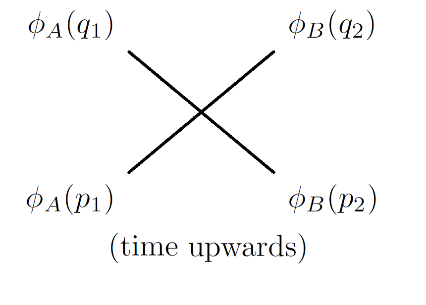
In Tree level we have,

Refer to caption
Figure 1: Tree-level interaction

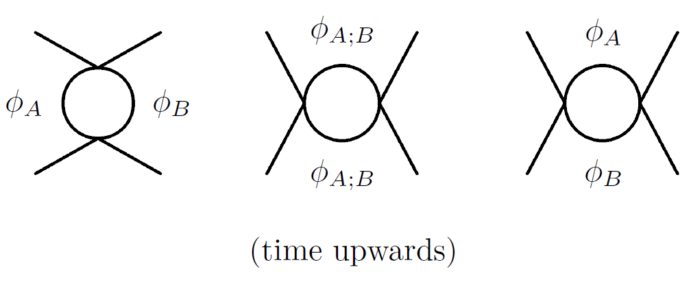
With 1-loop corrections we add the contributions shown in fig.2 , with the same asymptotic states as in fig.1,
Refer to caption
Figure 2: These the only three topologically different 1-loop diagrams that respect the coupling term in the Lagrangian. They are the s-channel, t-channel and u-channel, respectively.

We shall calculate the reduced density matrix for Alice in order to calculate the von Neumann entropy difference between the initial and final states. First we do this in Tree level, fig.1 and then add 1-loop corrections, represented by the s, t and u-channels seen in fig.2.

As usual we define the scattering amplitude \mathcal{M} as the matrix element

q1q2|iT^|p1p2quantum-operator-productsubscript𝑞1subscript𝑞2𝑖^𝑇subscript𝑝1subscript𝑝2\displaystyle\left<\right.\vec{q_{1}}\;\vec{q_{2}}\left.\right|i\hat{T}\left.\right|\vec{p_{1}}\;\vec{p_{2}}\left.\right> =\displaystyle= (2π)4δ(4)(p1+p2q1q2)superscript2𝜋4superscript𝛿4subscript𝑝1subscript𝑝2subscript𝑞1subscript𝑞2\displaystyle(2\pi)^{4}\delta^{(4)}(p_{1}+p_{2}-q_{1}-q_{2}) (8)
×\displaystyle\times i(p1,p2q1,q2),𝑖subscriptformulae-sequencesubscript𝑝1subscript𝑝2subscript𝑞1subscript𝑞2\displaystyle i\mathcal{M}_{(p_{1},p_{2}\rightarrow q_{1},q_{2})},

which is evaluated as

i=2iλRi(λR4π)2(u,t,s)+𝒪(λ3),𝑖2𝑖subscript𝜆𝑅𝑖superscriptsubscript𝜆𝑅4𝜋2𝑢𝑡𝑠𝒪superscript𝜆3i\mathcal{M}=-2i\lambda_{R}-i(\frac{\lambda_{R}}{4\pi})^{2}\mathcal{F}(u,t,s)+\mathcal{O}(\lambda^{3}), (9)

with (u,t,s)=4(3G(t)+2G(u)+G(s)+2)𝑢𝑡𝑠43𝐺𝑡2𝐺𝑢𝐺𝑠2\mathcal{F}(u,t,s)=4(3G(t)+2G(u)+G(s)+2), s=(p1+p2)2𝑠superscriptsubscript𝑝1subscript𝑝22s=(p_{1}+p_{2})^{2}, t=(p1q1)2𝑡superscriptsubscript𝑝1subscript𝑞12t=(p_{1}-q_{1})^{2} and u=(p1q2)2𝑢superscriptsubscript𝑝1subscript𝑞22u=(p_{1}-q_{2})^{2} being the Mandelstam variables and the function G(x)𝐺𝑥G(x) stands for

G(x)=2+14m2xln((14m2x+114m2x1)),𝐺𝑥214superscript𝑚2𝑥14superscript𝑚2𝑥114superscript𝑚2𝑥1G(x)=-2+\sqrt{1-\frac{4m^{2}}{x}}\ln{(\frac{\sqrt{1-\frac{4m^{2}}{x}}+1}{\sqrt{1-\frac{4m^{2}}{x}}-1})}, (10)

with x={t,u,s}𝑥𝑡𝑢𝑠x=\{t,u,s\}. We have adopted a renormalization condition where =2iλR2𝑖subscript𝜆𝑅\mathcal{M}=-2i\lambda_{R} at s=4m2𝑠4superscript𝑚2s=4m^{2} and t=u=0𝑡𝑢0t=u=0 in order to define the renormalized coupling constant λRsubscript𝜆𝑅\lambda_{R}, hereafter simply denoted by λ𝜆\lambda.

3 Alice’s reduced density matrix

3.1 Density operators and the Von Neumann Entropy of Entanglement

Von Neumann’s entropy of entanglement is known to be an unequivocal measure for bi-partite entanglement. With ρABsubscript𝜌𝐴𝐵\rho_{AB} denoting the density operator present in the composite space of Alice and Bob, the Entropy of Entanglement between Alice’s and Bob’s systems is, by definition

SE=Tr(ρAlogρA),subscript𝑆𝐸𝑇𝑟subscript𝜌𝐴subscript𝜌𝐴S_{E}=-Tr\left(\rho_{A}\log\rho_{A}\right), (11)

where ρAsubscript𝜌𝐴\rho_{A} is Alice’s reduced density operator

ρA=TrB(ρAB)=+d3n(2π)3n|BρAB|nB2En.\rho_{A}=Tr_{B}(\rho_{AB})=\int^{+\infty}_{-\infty}\frac{d^{3}\vec{n}}{(2\pi)^{3}}\frac{\left.\right<\vec{n}|_{B}\;\rho_{AB}\;\left.|\vec{n}\right>_{B}}{2E_{\vec{n}}}. (12)

In the case of a diagonal operator

SE=n=1(ρn)log(ρn)subscript𝑆𝐸superscriptsubscript𝑛1subscript𝜌𝑛subscript𝜌𝑛S_{E}=-\sum_{n=1}^{\infty}(\rho_{n})\log(\rho_{n}) (13)

ρnsubscript𝜌𝑛\rho_{n} represents the n𝑛nth element of the diagonal, with the density matrix elements in a momentum basis given by

ρnl=n|ρA|l2EnL32ElL3,\rho_{nl}=\frac{\left.\right<\vec{n}\left.\right|{{\rho}_{A}}\left.\right|\vec{l}\left.\right>}{\sqrt{2E_{\vec{n}}L^{3}}\sqrt{2E_{\vec{l}}L^{3}}}, (14)

where L3superscript𝐿3L^{3} is the phase space volume defined as L3=(2πδ(0))3superscript𝐿3superscript2𝜋𝛿03L^{3}=(2\pi\delta(0))^{3} which, just as the squared energy delta function, will be eliminated with a proper normalization, further on. We are interested in studying its variation during a scattering process,

ΔSE=SE(out)SE(in).Δsubscript𝑆𝐸subscript𝑆𝐸𝑜𝑢𝑡subscript𝑆𝐸𝑖𝑛\Delta S_{E}=S_{E\;(out)}-S_{E\;(in)}. (15)

The process to calculate it will be the following,

|ΨinρAB(in)ρA(in)SE(in)subscriptketΨ𝑖𝑛subscriptsuperscript𝜌𝑖𝑛𝐴𝐵subscriptsuperscript𝜌𝑖𝑛𝐴subscript𝑆𝐸𝑖𝑛\ket{\Psi}_{in}\rightarrow\rho^{(in)}_{AB}\rightarrow\rho^{(in)}_{A}\rightarrow S_{E\;(in)} (16)
|ΨoutρAB(out)ρA(out)SE(out)subscriptketΨ𝑜𝑢𝑡subscriptsuperscript𝜌𝑜𝑢𝑡𝐴𝐵subscriptsuperscript𝜌𝑜𝑢𝑡𝐴subscript𝑆𝐸𝑜𝑢𝑡\!\!\!\!\!\!\!\!\!\ket{\Psi}_{out}\rightarrow\rho^{(out)}_{AB}\rightarrow\rho^{(out)}_{A}\rightarrow S_{E\;(out)}

and obviously in the end use (eq.15).

3.2 When the in state” is separable

In this case we define the state as

|Ψin=|p1,p2=|p1A|p2B,subscriptketΨ𝑖𝑛ketsubscript𝑝1subscript𝑝2tensor-productsubscriptketsubscript𝑝1𝐴subscriptketsubscript𝑝2𝐵\ket{\Psi}_{in}=\ket{\vec{p_{1}},\vec{p_{2}}}=\ket{\vec{p_{1}}}_{A}\otimes\ket{\vec{p_{2}}}_{B}, (17)

Following the recipe of (eq.16), one realizes that since the initial state is separable, by definition, the entropy of entanglement vanishes before the collision, and (eq.15) becomes just SE(out)subscript𝑆𝐸𝑜𝑢𝑡S_{E\;(out)}.

We shall work in the center-of-mass (CM) frame in which the in-state is given by |p1,p1ketsubscript𝑝1subscript𝑝1\ket{\vec{p_{1}},-\vec{p_{1}}} and a general out-state can be written as

|(q1,q2)=cp1|(p1,p1)+kp1ck|(k,k),ketsubscript𝑞1subscript𝑞2subscript𝑐subscript𝑝1ketsubscript𝑝1subscript𝑝1subscriptfor-all𝑘subscript𝑝1subscript𝑐𝑘ket𝑘𝑘\ket{(\vec{q_{1}},\vec{q_{2}})}=c_{\vec{p_{1}}}\ket{(\vec{p_{1}},-\vec{p_{1}})}+\sum_{\forall\vec{k}\neq{\vec{p_{1}}}}c_{\vec{k}}|(\vec{k},-\vec{k})\rangle,

the parenthesis meaning that the out-state is generally entangled in the momenta. It is calculated using (5) and (8) as

|Ψout=|p1p2+q1p1;q2p2|q1q2q1q2|iT^|p1p22Eq12Eq2,subscriptketΨ𝑜𝑢𝑡ketsubscript𝑝1subscript𝑝2subscriptdouble-integralformulae-sequencesubscript𝑞1subscript𝑝1subscript𝑞2subscript𝑝2ketsubscript𝑞1subscript𝑞2quantum-operator-productsubscript𝑞1subscript𝑞2𝑖^𝑇subscript𝑝1subscript𝑝22subscript𝐸subscript𝑞12subscript𝐸subscript𝑞2\ket{\Psi}_{out}=|\vec{p_{1}}\;\vec{p_{2}}\left.\right>+\!\!\!\!\!\!\!\!\iint\limits_{\vec{q_{1}}\neq\vec{p_{1}};\\ \vec{q_{2}}\neq\vec{p_{2}}}\frac{|\vec{q_{1}}\;\vec{q_{2}}\left.\right>\left<\right.\vec{q_{1}}\;\vec{q_{2}}\left.\right|i\hat{T}\left.\right|\vec{p_{1}}\;\vec{p_{2}}\left.\right>}{2E_{\vec{q_{1}}}{2E_{\vec{q_{2}}}}},\\ (18)
=\displaystyle= |p1p2+q1p1q2p2(2π)4δ(4)(p1+p2q1q2)2Eq12Eq2ketsubscript𝑝1subscript𝑝2subscriptdouble-integralsubscript𝑞1subscript𝑝1subscript𝑞2subscript𝑝2superscript2𝜋4superscript𝛿4subscript𝑝1subscript𝑝2subscript𝑞1subscript𝑞22subscript𝐸subscript𝑞12subscript𝐸subscript𝑞2\displaystyle|\vec{p_{1}}\;\vec{p_{2}}\left.\right>+\iint\limits_{\vec{q_{1}}\neq\vec{p_{1}}\vec{q_{2}}\neq\vec{p_{2}}}\frac{(2\pi)^{4}\delta^{(4)}(p_{1}+p_{2}-q_{1}-q_{2})}{2E_{\vec{q_{1}}}{2E_{\vec{q_{2}}}}} (19)
×\displaystyle\times i(p1p2q1q2)|q1q2𝑖subscriptsubscript𝑝1subscript𝑝2subscript𝑞1subscript𝑞2ketsubscript𝑞1subscript𝑞2\displaystyle i\mathcal{M}_{(p_{1}p_{2}\rightarrow q_{1}q_{2})}|\vec{q_{1}}\;\vec{q_{2}}\left.\right>

with pd3p/(2π)3subscript𝑝superscript𝑑3𝑝superscript2𝜋3\int_{\vec{p}}\equiv\int d^{3}\vec{p}/(2\pi)^{3} and we normalize the inner product as q|p=2Eq(2π)3δ(3)(qp)inner-product𝑞𝑝2subscript𝐸𝑞superscript2𝜋3superscript𝛿3𝑞𝑝\langle\vec{q}|\vec{p}\rangle=2E_{\vec{q}}(2\pi)^{3}\delta^{(3)}(\vec{q}-\vec{p}). Moreover we separate the δ(4)superscript𝛿4\delta^{(4)} into δ(3)(p1+p2q1q2)δ(Ep1+Ep2Eq1Eq2)superscript𝛿3subscript𝑝1subscript𝑝2subscript𝑞1subscript𝑞2𝛿subscript𝐸subscript𝑝1subscript𝐸subscript𝑝2subscript𝐸subscript𝑞1subscript𝐸subscript𝑞2\delta^{(3)}(\vec{p_{1}}+\vec{p_{2}}-\vec{q_{1}}-\vec{q_{2}})\delta(E_{\vec{p_{1}}}+E_{\vec{p_{2}}}-E_{\vec{q_{1}}}-E_{\vec{q_{2}}}). Consequently,

|Ψout=|p1p2+q1p1|q1,p1+p2q1[(2π)δ(E)]i2Eq12Ep1+p2q1,subscriptketΨ𝑜𝑢𝑡ketsubscript𝑝1subscript𝑝2subscriptsubscript𝑞1subscript𝑝1ketsubscript𝑞1subscript𝑝1subscript𝑝2subscript𝑞1delimited-[]2𝜋𝛿𝐸𝑖2subscript𝐸subscript𝑞12subscript𝐸subscript𝑝1subscript𝑝2subscript𝑞1\ket{\Psi}_{out}=|\vec{p_{1}}\;\vec{p_{2}}\left.\right>+\!\!\!\int\limits_{\vec{q_{1}}\neq\vec{p_{1}}}\frac{|\vec{q_{1}},\;\vec{p_{1}}+\vec{p_{2}}-\vec{q_{1}}\left.\right>[(2\pi)\delta(E)]i\mathcal{M}}{2E_{\vec{q_{1}}}2E_{\vec{p_{1}}+\vec{p_{2}}-\vec{q_{1}}}}, (20)

in which δ(E)𝛿𝐸\delta(E) stands for δ(Ep1+Ep2Eq1Ep1+p2q1)𝛿subscript𝐸subscript𝑝1subscript𝐸subscript𝑝2subscript𝐸subscript𝑞1subscript𝐸subscript𝑝1subscript𝑝2subscript𝑞1\delta(E_{\vec{p_{1}}}+E_{\vec{p_{2}}}-E_{\vec{q_{1}}}-E_{\vec{p_{1}}+\vec{p_{2}}-\vec{q_{1}}}) and \mathcal{M} is evaluated with four-momentum
q2=(Ep1+p2q1,p1+p2q1)subscript𝑞2subscript𝐸subscript𝑝1subscript𝑝2subscript𝑞1subscript𝑝1subscript𝑝2subscript𝑞1q_{2}=(E_{\vec{p_{1}}+\vec{p_{2}}-\vec{q_{1}}},\vec{p_{1}}+\vec{p_{2}}-\vec{q_{1}}). From (20) we can evaluate

ρ^out=|ΨoutoutΨ|,\hat{\rho}_{out}=|\Psi\rangle_{out}\,\,{}_{out}\langle\Psi|,

as well as the reduced density matrix for Alice, integrating out the momenta of Bob, p2subscript𝑝2\vec{p_{2}}. Explicitly,

ρ^A=|p1p1|(2Ep2L3)+qp1|qq|[(2π)δ(E)]2||2(2Eq)22Ep1+p2q.\hat{\rho}_{A}=\left.\right|\vec{p_{1}}\left.\right>\left.\right<\vec{p_{1}}\left.\right|(2E_{\vec{p_{2}}}L^{3})+\int\limits_{\vec{q}\neq\vec{p_{1}}}\frac{\left.\right|\vec{q}\left.\right>\left.\right<\vec{q}\left.\right|[(2\pi)\delta(E)]^{2}|\mathcal{M}|^{2}}{(2E_{\vec{q}})^{2}2E_{\vec{p_{1}}+\vec{p_{2}}-\vec{q}}}. (21)

In order to compute the reduced density matrix let us split (t,u,s)𝑡𝑢𝑠\mathcal{F}(t,u,s) in equation (9) into real and imaginary parts. Hence

||2=4λ2+4λ(λ4π)2Re[]+(λ4π)4(Re2[]+Im2[])superscript24superscript𝜆24𝜆superscript𝜆4𝜋2Redelimited-[]superscript𝜆4𝜋4superscriptRe2delimited-[]superscriptIm2delimited-[]|\mathcal{M}|^{2}=4\lambda^{2}+4\lambda(\frac{\lambda}{4\pi})^{2}\textrm{Re}[\mathcal{F}]+(\frac{\lambda}{4\pi})^{4}\big{(}\textrm{Re}^{2}[\mathcal{F}]+\textrm{Im}^{2}[\mathcal{F}]\big{)} (22)

which enables us to write

ρ^A=|p1p1|(2Ep2L3)+2+3+4,\hat{\rho}_{A}=\left.\right|\vec{p_{1}}\left.\right>\left.\right<\vec{p_{1}}\left.\right|(2E_{\vec{p_{2}}}L^{3})+\mathcal{I}_{2}+\mathcal{I}_{3}+\mathcal{I}_{4}, (23)

with

2qp1|qq|[(2π)δ(E)]2(2Eq)22Ep1+p2q(4λ2),\mathcal{I}_{2}\equiv\int\limits_{\vec{q}\neq\vec{p_{1}}}\frac{\left.\right|\vec{q}\left.\right>\left.\right<\vec{q}\left.\right|[(2\pi)\delta(E)]^{2}}{(2E_{\vec{q}})^{2}2E_{\vec{p_{1}}+\vec{p_{2}}-\vec{q}}}(4\lambda^{2}),
3qp1|qq|[(2π)δ(E)]2(2Eq)22Ep1+p2q(4λ(λ4π)2Re[]),\mathcal{I}_{3}\equiv\int\limits_{\vec{q}\neq\vec{p_{1}}}\frac{\left.\right|\vec{q}\left.\right>\left.\right<\vec{q}\left.\right|[(2\pi)\delta(E)]^{2}}{(2E_{\vec{q}})^{2}2E_{\vec{p_{1}}+\vec{p_{2}}-\vec{q}}}(4\lambda(\frac{\lambda}{4\pi})^{2}\textrm{Re}[\mathcal{F}]),
4qp1|qq|[(2π)δ(E)]2(2Eq)22Ep1+p2q(λ4π)4(Re2[]+Im2[]).\mathcal{I}_{4}\equiv\int\limits_{\vec{q}\neq\vec{p_{1}}}\frac{\left.\right|\vec{q}\left.\right>\left.\right<\vec{q}\left.\right|[(2\pi)\delta(E)]^{2}}{(2E_{\vec{q}})^{2}2E_{\vec{p_{1}}+\vec{p_{2}}-\vec{q}}}(\frac{\lambda}{4\pi})^{4}(\textrm{Re}^{2}[\mathcal{F}]+\textrm{Im}^{2}[\mathcal{F}]).

We normalize the reduced density operator by demanding that TrA(𝒩ρ^A)=TrA(ρ^An)=1𝑇subscript𝑟𝐴𝒩subscript^𝜌𝐴𝑇subscript𝑟𝐴superscriptsubscript^𝜌𝐴𝑛1Tr_{A}(\mathcal{N}\hat{\rho}_{A})=Tr_{A}(\hat{\rho}_{A}^{n})=1 which amounts to requiring that

𝒩+d3n(2π)3n|ρ^A|n2En=1.\mathcal{N}\int^{+\infty}_{-\infty}\frac{d^{3}\vec{n}}{(2\pi)^{3}}\frac{\left.\right<\vec{n}|\;\hat{\rho}_{A}\left.|\vec{n}\right>}{2E_{\vec{n}}}=1. (24)

Setting

+d3n(2π)3n|i|n2Eni,i=2,3,4,\int^{+\infty}_{-\infty}\frac{d^{3}\vec{n}}{(2\pi)^{3}}\frac{\left.\right<\vec{n}|\;\mathcal{I}_{i}\left.|\vec{n}\right>}{2E_{\vec{n}}}\equiv\langle\mathcal{I}_{i}\rangle\,\,\,,\,\,i=2,3,4, (25)

yields

𝒩=[(2Ep1L3)(2Ep2L3)+2+3+4]1𝒩superscriptdelimited-[]2subscript𝐸subscript𝑝1superscript𝐿32subscript𝐸subscript𝑝2superscript𝐿3delimited-⟨⟩subscript2delimited-⟨⟩subscript3delimited-⟨⟩subscript41\mathcal{N}=[(2E_{\vec{p_{1}}}L^{3})(2E_{\vec{p_{2}}}L^{3})+\langle\mathcal{I}_{2}\rangle+\langle\mathcal{I}_{3}\rangle+\langle\mathcal{I}_{4}\rangle]^{-1}

and the renormalized density operator to one loop order formally reads

ρ^A=|p1p1|(2Ep2L3)+2+3+4(2Ep1L3)(2Ep2L3)+2+3+4,subscript^𝜌𝐴ketsubscript𝑝1brasubscript𝑝12subscript𝐸subscript𝑝2superscript𝐿3subscript2subscript3subscript42subscript𝐸subscript𝑝1superscript𝐿32subscript𝐸subscript𝑝2superscript𝐿3delimited-⟨⟩subscript2delimited-⟨⟩subscript3delimited-⟨⟩subscript4\hat{\rho}_{A}=\frac{|\vec{p_{1}}\rangle\langle\vec{p_{1}}|(2E_{\vec{p_{2}}}L^{3})+\mathcal{I}_{2}+\mathcal{I}_{3}+\mathcal{I}_{4}}{(2E_{\vec{p_{1}}}L^{3})(2E_{\vec{p_{2}}}L^{3})+\langle\mathcal{I}_{2}\rangle+\langle\mathcal{I}_{3}\rangle+\langle\mathcal{I}_{4}\rangle}, (26)

where we have dropped the superscript n𝑛n for brevity. Notice that 3subscript3\mathcal{I}_{3} and 4subscript4\mathcal{I}_{4} represent the one loop correction to the scattering amplitude.

4 Transition amplitude in CM variables

In the CM frame we have Ep1=Ep2ECMsubscript𝐸subscript𝑝1subscript𝐸subscript𝑝2subscript𝐸𝐶𝑀E_{\vec{p_{1}}}=E_{\vec{p_{2}}}\equiv E_{CM}, p1=p2|p1|=|p2||pCM|subscript𝑝1subscript𝑝2subscript𝑝1subscript𝑝2subscript𝑝𝐶𝑀\vec{p_{1}}=-\vec{p_{2}}\rightarrow|\vec{p_{1}}|=|\vec{p_{2}}|\equiv|\vec{p}_{CM}| and the energy delta function δ(E)𝛿𝐸\delta(E) becomes δ(2ECM2Eq)𝛿2subscript𝐸𝐶𝑀2subscript𝐸𝑞\delta(2E_{CM}-2E_{\vec{q}}). Hence, the Mandelstam variables in the one loop correction to the transition amplitude in equation (9) read, in the CM coordinates,

uCMsubscript𝑢𝐶𝑀\displaystyle u_{CM} =\displaystyle= 2pCM2(1+cosθ),2subscriptsuperscript𝑝2𝐶𝑀1𝜃\displaystyle-2p^{2}_{CM}(1+\cos\theta),
tCMsubscript𝑡𝐶𝑀\displaystyle t_{CM} =\displaystyle= 2pCM2(1cosθ)and2subscriptsuperscript𝑝2𝐶𝑀1𝜃and\displaystyle-2p^{2}_{CM}(1-\cos\theta)\,\,\,\mathrm{and}
sCMsubscript𝑠𝐶𝑀\displaystyle s_{CM} =\displaystyle= 4(m2+pCM2),4superscript𝑚2subscriptsuperscript𝑝2𝐶𝑀\displaystyle 4(m^{2}+p^{2}_{CM}), (27)

θ𝜃\theta being the scattering angle. Using equations (9), (10) and (27), the real and the imaginary parts of \mathcal{F} become a function of the velocity and the scattering angle in the CM frame, (p,θ)𝑝𝜃{\cal F}(\vec{p},\theta), namely

Re[]=12G(2p2(1+cosθ))+8G(2p2(1cosθ))Redelimited-[]12𝐺2superscript𝑝21𝜃8𝐺2superscript𝑝21𝜃\textrm{Re}[\mathcal{F}]=12G\left(-2p^{2}\cdot(1+\cos\theta)\right)+8G\left(-2p^{2}\cdot(1-\cos\theta)\right) (28)
+4|vp|log((1+|vp|1|vp|));Im[]=4π(|vp|);4subscript𝑣𝑝1subscript𝑣𝑝1subscript𝑣𝑝Imdelimited-[]4𝜋subscript𝑣𝑝\!\!+4|v_{\vec{p}}|\log{\left(\frac{1+|v_{\vec{p}}|}{1-|v_{\vec{p}}|}\right)};\;\;\;\;\textrm{Im}[\mathcal{F}]=4\pi(|v_{\vec{p}}|);

where we use the shorthand notation pCMpsubscript𝑝𝐶𝑀𝑝\vec{p}_{CM}\equiv\vec{p}, and vpsubscript𝑣𝑝v_{\vec{p}} stands for the CM velocity.

4.1 Tree-level

First we calculate tree-level result for the entanglement entropy, from ||2=4λ2superscript24superscript𝜆2|\mathcal{M}|^{2}=4\lambda^{2}.

For this case eq. (26) reduces to

ρA(n)=|pp|(2EpL3)+2(2EpL3)2+2{\rho_{A}}^{(n)}=\frac{\left.\right|\vec{p}\left.\right>\left.\right<\vec{p}\left.\right|(2E_{\vec{p}}L^{3})+\mathcal{I}_{2}}{(2E_{\vec{p}}L^{3})^{2}+\langle\mathcal{I}_{2}\rangle} (29)
=|pp|(2EpL3)(1+𝒜tree)+2(2EpL3)2(1+𝒜tree).=\frac{\left.\right|\vec{p}\left.\right>\left.\right<\vec{p}\left.\right|}{(2E_{\vec{p}}L^{3})(1+\mathcal{A}_{tree})}+\frac{\mathcal{I}_{2}}{(2E_{\vec{p}}L^{3})^{2}(1+\mathcal{A}_{tree})}.

where

𝒜tree=2(2EpL3)2subscript𝒜𝑡𝑟𝑒𝑒delimited-⟨⟩subscript2superscript2subscript𝐸𝑝superscript𝐿32\mathcal{A}_{tree}=\frac{\langle\mathcal{I}_{2}\rangle}{(2E_{\vec{p}}L^{3})^{2}}

which yields in the CM

𝒜tree=λ28π|vp|(EpL)2subscript𝒜𝑡𝑟𝑒𝑒superscript𝜆28𝜋subscript𝑣𝑝superscriptsubscript𝐸𝑝𝐿2\mathcal{A}_{tree}=\frac{\lambda^{2}}{8\pi}\frac{|v_{\vec{p}}|}{(E_{\vec{p}}L)^{2}}

We can now calculate the entropy associated with the state after the collision, by applying (eq.12), or since we know the matrix is diagonal (eq.11),

(SE)tree=ρplog(ρp)L3(2π)3+(ρklogρk)𝑑k,kp.formulae-sequencesubscriptsubscript𝑆𝐸𝑡𝑟𝑒𝑒subscript𝜌𝑝subscript𝜌𝑝superscript𝐿3superscript2𝜋3subscriptsuperscriptsubscript𝜌𝑘subscript𝜌𝑘differential-d𝑘𝑘𝑝(S_{E})_{tree}=-\rho_{p}\log{\rho_{p}}-\frac{L^{3}}{(2\pi)^{3}}\int^{+\infty}_{-\infty}(\rho_{k}\log\rho_{k})d\vec{k},k\neq p. (30)

We can easily compute ρpsubscript𝜌𝑝\rho_{p} and ρksubscript𝜌𝑘\rho_{k} by using (eq.14) and (eq.29),

ρp=11+𝒜tree;ρk=(2πδ(2Ep2Ek)2Ek2EpL3)24λ21+𝒜tree.formulae-sequencesubscript𝜌𝑝11subscript𝒜𝑡𝑟𝑒𝑒subscript𝜌𝑘superscript2𝜋𝛿2subscript𝐸𝑝2subscript𝐸𝑘2subscript𝐸𝑘2subscript𝐸𝑝superscript𝐿324superscript𝜆21subscript𝒜𝑡𝑟𝑒𝑒\rho_{p}=\frac{1}{1+\mathcal{A}_{tree}};\;\;\rho_{k}=\left(\frac{2\pi\delta(2E_{\vec{p}}-2E_{\vec{k}})}{2E_{\vec{k}}2E_{\vec{p}}L^{3}}\right)^{2}\frac{4\lambda^{2}}{1+\mathcal{A}_{tree}}.

Substituting into (eq.30) and solving the integral in the second term we have,

(SE)tree=log((1+𝒜tree))1+𝒜tree+λ2|vp|log(((4E¯p4(1+𝒜tree))/λ2))4E¯p2(1+𝒜tree),subscriptsubscript𝑆𝐸𝑡𝑟𝑒𝑒1subscript𝒜𝑡𝑟𝑒𝑒1subscript𝒜𝑡𝑟𝑒𝑒superscript𝜆2subscript𝑣𝑝4superscriptsubscript¯𝐸𝑝41subscript𝒜𝑡𝑟𝑒𝑒superscript𝜆24superscriptsubscript¯𝐸𝑝21subscript𝒜𝑡𝑟𝑒𝑒(S_{E})_{tree}=\frac{\log{(1+\mathcal{A}_{tree})}}{1+\mathcal{A}_{tree}}+\lambda^{2}|v_{\vec{p}}|\frac{\log{\left((4\bar{E}_{\vec{p}}^{4}(1+\mathcal{A}_{tree}))/\lambda^{2}\right)}}{4\bar{E}_{\vec{p}}^{2}(1+\mathcal{A}_{tree})}, (31)

E¯psubscript¯𝐸𝑝\bar{E}_{\vec{p}} is defined to be EpL=γpm¯subscript𝐸𝑝𝐿subscript𝛾𝑝¯𝑚{E}_{\vec{p}}L=\gamma_{\vec{p}}\;\bar{m}, if m¯=mL¯𝑚𝑚𝐿\bar{m}=mL.

It is worth mentioning that this result is equivalent to the similiar result obtained in [19].

4.2 1-Loop corrections

In a similar way one obtains up to 1-Loop, the following normalized reduced density operator

ρA(n)=|pp|(2EpL3)(1+𝒜1loop)+{\rho_{A}}^{(n)}=\frac{\left.\right|\vec{p}\left.\right>\left.\right<\vec{p}\left.\right|}{(2E_{\vec{p}}L^{3})(1+\mathcal{A}_{1loop})}+ (32)
1(1+𝒜1loop)(2(2EpL3)2+3(2EpL3)2+4(2EpL3)2)11subscript𝒜1𝑙𝑜𝑜𝑝subscript2superscript2subscript𝐸𝑝superscript𝐿32subscript3superscript2subscript𝐸𝑝superscript𝐿32subscript4superscript2subscript𝐸𝑝superscript𝐿32\frac{1}{(1+\mathcal{A}_{1loop})}\left(\frac{\mathcal{I}_{2}}{{(2E_{\vec{p}}L^{3})^{2}}}+\frac{\mathcal{I}_{3}}{{(2E_{\vec{p}}L^{3})^{2}}}+\frac{\mathcal{I}_{4}}{{(2E_{\vec{p}}L^{3})^{2}}}\right)

where

𝒜1loop=2(2EpL3)2+3(2EpL3)2+4(2EpL3)2.subscript𝒜1𝑙𝑜𝑜𝑝delimited-⟨⟩subscript2superscript2subscript𝐸𝑝superscript𝐿32delimited-⟨⟩subscript3superscript2subscript𝐸𝑝superscript𝐿32delimited-⟨⟩subscript4superscript2subscript𝐸𝑝superscript𝐿32\mathcal{A}_{1loop}=\frac{\langle\mathcal{I}_{2}\rangle}{(2E_{\vec{p}}L^{3})^{2}}+\frac{\langle\mathcal{I}_{3}\rangle}{(2E_{\vec{p}}L^{3})^{2}}+\frac{\langle\mathcal{I}_{4}\rangle}{(2E_{\vec{p}}L^{3})^{2}}.

Explicitly the integrals read

3=L44πλ(λ4π)2|vp|(120+log(1/|vp|+11/|vp|1)(40|vp|)+\langle\mathcal{I}_{3}\rangle=\frac{L^{4}}{4\pi}\lambda(\frac{\lambda}{4\pi})^{2}|v_{\vec{p}}|(-120+\log{\frac{1/|v_{\vec{p}}|+1}{1/|v_{\vec{p}}|-1}}\left(\frac{40}{|v_{\vec{p}}|}\right)+ (33)
+(10vp210)(log(1/|vp|+11/|vp|1))2+8|vp|log1+|vp|1|vp|),+(\frac{10}{v^{2}_{\vec{p}}}-10)\left(\log{\frac{1/|v_{\vec{p}}|+1}{1/|v_{\vec{p}}|-1}}\right)^{2}+8|v_{\vec{p}}|\log\frac{1+|v_{\vec{p}}|}{1-|v_{\vec{p}}|}),

and

4=L416π(λ4π)4|vp|(0π(Re[])2sinθdθ+32π2vp2),delimited-⟨⟩subscript4superscript𝐿416𝜋superscript𝜆4𝜋4subscript𝑣𝑝subscriptsuperscript𝜋0superscriptRedelimited-[]2𝜃𝑑𝜃32superscript𝜋2subscriptsuperscript𝑣2𝑝\langle\mathcal{I}_{4}\rangle=\frac{L^{4}}{16\pi}(\frac{\lambda}{4\pi})^{4}|v_{\vec{p}}|\left(\int^{\pi}_{0}(\textrm{Re}[\mathcal{F}])^{2}\sin\theta d\theta+32\pi^{2}v^{2}_{\vec{p}}\right), (34)

which is computed numerically.

Again we calculate ρpsubscript𝜌𝑝\rho_{p} and ρksubscript𝜌𝑘\rho_{k} by using (eq.14) and now (eq.32) ,

ρp=11+𝒜1loop;ρk=(2πδ(2Ep2Ek)2Ek2EpL3)2Ω(k,θ)1+𝒜1loop,formulae-sequencesubscript𝜌𝑝11subscript𝒜1𝑙𝑜𝑜𝑝subscript𝜌𝑘superscript2𝜋𝛿2subscript𝐸𝑝2subscript𝐸𝑘2subscript𝐸𝑘2subscript𝐸𝑝superscript𝐿32Ω𝑘superscript𝜃1subscript𝒜1𝑙𝑜𝑜𝑝\rho_{p}=\frac{1}{1+\mathcal{A}_{1loop}};\;\;\rho_{k}=\left(\frac{2\pi\delta(2E_{\vec{p}}-2E_{\vec{k}})}{2E_{\vec{k}}2E_{\vec{p}}L^{3}}\right)^{2}\frac{\Omega(\vec{k},\theta^{{}^{\prime}})}{1+\mathcal{A}_{1loop}},

where Ω(k,θ)Ω𝑘superscript𝜃\Omega({\vec{k}},\theta^{{}^{\prime}}) is given by the same expression as (22) , with (k,θ)𝑘superscript𝜃{\cal F}(\vec{k},\theta^{{}^{\prime}}), see (28). Substituting these elements into the entropy (eq.30) and integrating the deltas, we get to 1-loop,

(SE)1loop=log((1+𝒜1loop))(1+𝒜1loop)+subscriptsubscript𝑆𝐸1𝑙𝑜𝑜𝑝limit-from1subscript𝒜1𝑙𝑜𝑜𝑝1subscript𝒜1𝑙𝑜𝑜𝑝\displaystyle(S_{E})_{1-loop}=\frac{\log{{(1+\mathcal{A}_{1loop})}}}{(1+\mathcal{A}_{1loop})}+
|vp|/64π(E¯p)2(1+𝒜1loop)×\displaystyle\frac{|v_{\vec{p}}|/64\pi}{(\bar{E}_{\vec{p}})^{2}(1+\mathcal{A}_{1loop})}\times
0πsinθΩ(θ)log([16(E¯p)4(1+𝒜1loop)Ω(θ)]dθ).subscriptsuperscript𝜋0superscript𝜃Ωsuperscript𝜃delimited-[]16superscriptsubscript¯𝐸𝑝41subscript𝒜1𝑙𝑜𝑜𝑝Ωsuperscript𝜃𝑑superscript𝜃\displaystyle\int^{\pi}_{0}\sin\theta^{{}^{\prime}}\Omega(\theta^{{}^{\prime}})\log{[\frac{16(\bar{E}_{\vec{p}})^{4}(1+\mathcal{A}_{1loop})}{\Omega(\theta^{{}^{\prime}})}]d\theta^{{}^{\prime}}}. (35)

It should be noticed that if we take (eq.4.2) and take the limiting case when 𝒜1loop𝒜treesubscript𝒜1𝑙𝑜𝑜𝑝subscript𝒜𝑡𝑟𝑒𝑒\mathcal{A}_{1loop}\rightarrow\mathcal{A}_{tree} and Ω(θ)4λ2Ωsuperscript𝜃4superscript𝜆2\Omega(\theta^{{}^{\prime}})\rightarrow 4\lambda^{2} we reproduce (eq.31).

4.2.1 Graphical solutions

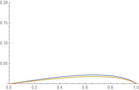
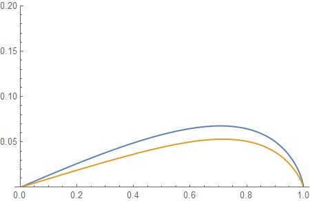
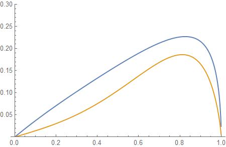
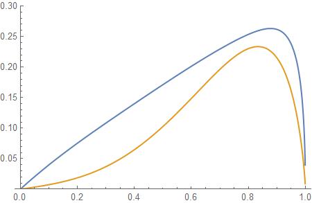
We take (eq.4.2), (eq.31), and choose m¯=1¯𝑚1\bar{m}=1. All the graphics are of the form (SE(S_{E} vs |vp|)|v_{\vec{p}}|). The Tree-level contribution is in orange and the Tree-level with the higher order corrections (up to 1-loop) is in blue.In fig. 3 we vary increasingly the value of the coupling λ𝜆\lambda, staying in the perturbative regime, i.e. the variations in the maxima of SEsubscript𝑆𝐸S_{E} between the Tree level plus 1-loop corrections and Tree level alone are required to be less than 30%percent3030\%.

Refer to caption
(a)
Refer to caption
(b)
Refer to caption
(c)
Refer to caption
(d)
Figure 3: SE(|vp|)subscript𝑆𝐸subscript𝑣𝑝S_{E}(|v_{\vec{p}}|) in Tree-level (orange) and 1-loop (blue), forλ𝜆\lambda=[0.5(top left), 1(top right), 2.5(bottom left), 3(bottom right)]

One sees that the velocity for the maximum value of the entropy increases with λ𝜆\lambda, actually it increases in an approximately linear way, as shown in fig. 4.
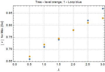
Refer to caption
Figure 4: |vp|subscript𝑣𝑝|v_{\vec{p}}| vs. λ𝜆\lambda

One can appreciate that the velocities in the 1-loop corrections at the maximum of entropy are only slightly different than the velocities in Tree-level.

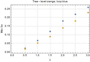
The variation of the entropy maximum as a function of λ𝜆\lambda is shown in fig. 5. Note that it is strongly dependent on the value of the coupling, one order of magnitude difference when read at λ=0.5𝜆0.5\lambda=0.5 and λ=3𝜆3\lambda=3.

Refer to caption
Figure 5: SEsubscript𝑆𝐸S_{E} vs. λ𝜆\lambda

4.3 When the before state is entangled

Now, in analogy to a typical Bell state, we propose the following simplest possible initial entagled state in a momentum basis, already seen from the perspective of the CM,

|Φin=αp|p,p+αk|k,k,{pk};subscriptketΦinsubscript𝛼𝑝ket𝑝𝑝subscript𝛼𝑘ket𝑘𝑘for-all𝑝𝑘\displaystyle\ket{\Phi}_{\textit{in}}=\alpha_{p}\ket{\vec{p},-\vec{p}}+\alpha_{k}\left.\right|\!\vec{k},-\vec{k}\!\left.\right>,\;\forall\left\{\vec{p}\neq\vec{k}\right\};
|αp|2+|αk|2=1.superscriptsubscript𝛼𝑝2superscriptsubscript𝛼𝑘21\displaystyle|\alpha_{p}|^{2}+|\alpha_{k}|^{2}=1. (36)

Following the recipe of (eq. 16), we now calculate the reduced operator and consequently the entropy associated with the initial state. Unlike the previous case it won’t be null.

Alice’s already normalized operator is given by,

ρA=|pp|(L3)(2Ep)(1+1/𝒞)+|kk|(L3)(2Ek)(1+𝒞),\rho_{A}=\frac{\ket{\vec{p}}\bra{\vec{p}}}{(L^{3})(2E_{\vec{p}})\left(1+1/\mathcal{C}\right)}+\frac{\left.\right|\!\vec{k}\!\left.\right>\left.\right<\!\vec{k}\!\left.\right|}{(L^{3})(2E_{\vec{k}})\left(1+\mathcal{C}\right)}, (37)

where 𝒞=|αp|2|αk|2(EpEk)2=|αp|2|αk|2(1vk21vp2)𝒞superscriptsubscript𝛼𝑝2superscriptsubscript𝛼𝑘2superscriptsubscript𝐸𝑝subscript𝐸𝑘2superscriptsubscript𝛼𝑝2superscriptsubscript𝛼𝑘21superscriptsubscript𝑣𝑘21superscriptsubscript𝑣𝑝2\mathcal{C}=\frac{|\alpha_{p}|^{2}}{|\alpha_{k}|^{2}}\left(\frac{E_{\vec{p}}}{E_{\vec{k}}}\right)^{2}=\frac{|\alpha_{p}|^{2}}{|\alpha_{k}|^{2}}\left(\frac{1-v_{\vec{k}}^{2}}{1-v_{\vec{p}}^{2}}\right).

We calculate the elements ρpsubscript𝜌𝑝\rho_{p} and ρksubscript𝜌𝑘\rho_{k}, by using (eq.14 again and inputting into (eq.30), we get for the initial state entanglement

SE=log((1+1/𝒞))1+1/𝒞+log((1+𝒞))1+𝒞S_{E}=\frac{\log{(1+1/\mathcal{C}})}{1+1/\mathcal{C}}+\frac{\log{(1+\mathcal{C}})}{1+\mathcal{C}} (38)

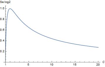
It can be easily seen that the entropy is maximum for 𝒞=1𝒞1\mathcal{C}=1, that represents the case of maximum entanglement. One can appreciate that for any choice of non null values of αpsubscript𝛼𝑝\alpha_{p} and αksubscript𝛼𝑘\alpha_{k} we can get a maximum entangled state for an appropriate choice of velocities values. This becomes evident if we take the condition for maximum entanglement,

|αp|2|αk|2(1vk21vp2)=1,superscriptsubscript𝛼𝑝2superscriptsubscript𝛼𝑘21superscriptsubscript𝑣𝑘21superscriptsubscript𝑣𝑝21\frac{|\alpha_{p}|^{2}}{|\alpha_{k}|^{2}}\left(\frac{1-v_{\vec{k}}^{2}}{1-v_{\vec{p}}^{2}}\right)=1,

and rewrite it as,

(1|αp|2)(1vp2)+|αp|2(vk21)=0,|αp|2(0,1)formulae-sequence1superscriptsubscript𝛼𝑝21superscriptsubscript𝑣𝑝2superscriptsubscript𝛼𝑝2superscriptsubscript𝑣𝑘210superscriptsubscript𝛼𝑝201(1-|\alpha_{p}|^{2})(1-v_{\vec{p}}^{2})+|\alpha_{p}|^{2}(v_{\vec{k}}^{2}-1)=0,\;|\alpha_{p}|^{2}\in(0,1)

This is the equation of a line segment between two points, one is negative (vk21superscriptsubscript𝑣𝑘21v_{\vec{k}}^{2}-1) and the other one is positive (1vp21superscriptsubscript𝑣𝑝21-v_{\vec{p}}^{2}), so regardless what their values are there is always one value of |αp|2superscriptsubscript𝛼𝑝2|\alpha_{p}|^{2} where the line passes trough the origin, hence the condition of maximum entangled is satisfied. For |αp|2=|αk|2=0.5superscriptsubscript𝛼𝑝2superscriptsubscript𝛼𝑘20.5|\alpha_{p}|^{2}=|\alpha_{k}|^{2}=0.5, this point is when |vp|=|vk|subscript𝑣𝑝subscript𝑣𝑘|v_{\vec{p}}|=|v_{\vec{k}}|.

The plot of (eq.38) as a function of 𝒞𝒞\mathcal{C} is

Refer to caption
Figure 6: SEsubscript𝑆𝐸S_{E}(𝒞𝒞\mathcal{C}). One can notice that for values where 𝒞𝒞\mathcal{C} goes to infinity or to zero the entropy vanishes (separable case), this being equivalent as to making one of the coefficients null.

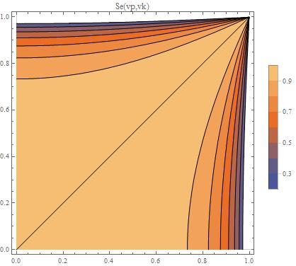
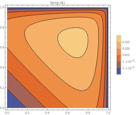
If instead of the initial two-state entanglement in a continuous momentum variable one would have taken a discrete two parameter state, as a Bell state of spins, the curve would e symmetric around the maximum. In fig. 7 we display the contour plot of SE(|vp|,|vk|)subscript𝑆𝐸subscript𝑣𝑝subscript𝑣𝑘S_{E}(|v_{\vec{p}}|,|v_{\vec{k}}|), for |αp|2=|αk|2=0.5superscriptsubscript𝛼𝑝2superscriptsubscript𝛼𝑘20.5|\alpha_{p}|^{2}=|\alpha_{k}|^{2}=0.5.

Refer to caption
Figure 7: All the points in the diagonal line |vp|=|vk|subscript𝑣𝑝subscript𝑣𝑘|v_{\vec{p}}|=|v_{\vec{k}}| correspond to the peak of maximum entropy in fig.6 when 𝒞=1𝒞1\mathcal{C}=1. This is easily understood since for every point of equal velocity when the coefficients are the same the ratio is always 1.

Now that we have concluded the study of the entropy before the collision we evaluate the entropy after the collision. We compute the sate after the collision by taking (eq.4.3) projecting it into a basis of momenta like in (eq.18) and applying (eq.5). Then we can construct the density operator and calculate Alice’s reduced density operator, following the steps in the recipe (eq.16).

The normalized operator in Tree-level when |αp|2=|αk|2=0.5superscriptsubscript𝛼𝑝2superscriptsubscript𝛼𝑘20.5|\alpha_{p}|^{2}=|\alpha_{k}|^{2}=0.5 takes the form,

ρA=𝒩(|pp|(2Ep)+|kk|(2Ek)+\rho_{A}=\mathcal{N}(\ket{\vec{p}}\bra{\vec{p}}(2E_{\vec{p}})+|\vec{k}\left.\right>\!\!\left.\right<\vec{k}|(2E_{\vec{k}})+ (39)
+4λ2{qp,k}d3q(2π)3|qq|(2Eq)3(2πδ(2EpCM2Eq))2+limit-from4superscript𝜆2subscript𝑞𝑝𝑘superscript𝑑3𝑞superscript2𝜋3ket𝑞bra𝑞superscript2subscript𝐸𝑞3superscript2𝜋𝛿2subscript𝐸subscript𝑝𝐶𝑀2subscript𝐸𝑞2+4\lambda^{2}\!\!\!\!\!\!\!\!\int\limits_{\left\{\vec{q}\neq\vec{p},\vec{k}\right\}}\!\!\!\!\frac{d^{3}\vec{q}}{(2\pi)^{3}}\frac{\ket{\vec{q}}\bra{\vec{q}}}{(2E_{\vec{q}})^{3}}\left(2\pi{\delta}(2E_{\vec{p}_{CM}}-2E_{\vec{q}})\right)^{2}+
+4λ2{qp,k}d3q(2π)3|qq|(2Eq)3(2πδ(2Ek2Eq))2).+4\lambda^{2}\!\!\!\!\!\!\!\int\limits_{\left\{\vec{q}\neq\vec{p},\vec{k}\right\}}\!\!\!\!\frac{d^{3}\vec{q}}{(2\pi)^{3}}\frac{\ket{\vec{q}}\bra{\vec{q}}}{(2E_{\vec{q}})^{3}}\left(2\pi{\delta}(2E_{\vec{k}}-2E_{\vec{q}})\right)^{2}).

Where 𝒩𝒩\mathcal{N} is calculated to be,

𝒩=1(2EpL3)2+(2EkL3)2+λ22πL4(|vp|+|vk|)𝒩1superscript2subscript𝐸𝑝superscript𝐿32superscript2subscript𝐸𝑘superscript𝐿32superscript𝜆22𝜋superscript𝐿4subscript𝑣𝑝subscript𝑣𝑘\mathcal{N}=\frac{1}{(2E_{\vec{p}}L^{3})^{2}+(2E_{\vec{k}}L^{3})^{2}+\frac{\lambda^{2}}{2\pi}L^{4}(|v_{\vec{p}}|+|v_{\vec{k}}|)}

Now the entropy has one more element adding to the remaining infinite amount, such that the entropy becomes,

(SE)out=ρplog(ρp)ρklog(ρk)L3(2π)3+ρnlog(ρn)𝑑nsubscriptsubscript𝑆𝐸𝑜𝑢𝑡subscript𝜌𝑝subscript𝜌𝑝subscript𝜌𝑘subscript𝜌𝑘superscript𝐿3superscript2𝜋3superscriptsubscriptsubscript𝜌𝑛subscript𝜌𝑛differential-d𝑛\left(S_{E}\right)_{out}=-\rho_{p}\log{\rho_{p}}-\rho_{k}\log{\rho_{k}}-\frac{L^{3}}{(2\pi)^{3}}\int_{-\infty}^{+\infty}\rho_{n}\log{\rho_{n}}dn (40)

Finding the elements in the usual way,

ρp=11+1𝒞+λ28πE¯p(|vp|+|vk|),subscript𝜌𝑝111𝒞superscript𝜆28𝜋subscript¯𝐸𝑝subscript𝑣𝑝subscript𝑣𝑘\rho_{p}=\frac{1}{1+\frac{1}{\mathcal{C}}+\frac{\lambda^{2}}{8\pi\bar{E}_{\vec{p}}}(|v_{\vec{p}}|+|v_{\vec{k}}|)},
ρk=11+𝒞+λ28πE¯k(|vp|+|vk|).subscript𝜌𝑘11𝒞superscript𝜆28𝜋subscript¯𝐸𝑘subscript𝑣𝑝subscript𝑣𝑘\rho_{k}=\frac{1}{1+\mathcal{C}+\frac{\lambda^{2}}{8\pi\bar{E}_{\vec{k}}}(|v_{\vec{p}}|+|v_{\vec{k}}|)}.

And finally,

ρn=(2π)2(δ2(2Ep2En)+δ2(2Ek2En))L6(2En)2((2Ek)2+(2Ep)2+λ22πL2(|vp|+|vk|))subscript𝜌𝑛superscript2𝜋2superscript𝛿22subscript𝐸𝑝2subscript𝐸𝑛superscript𝛿22subscript𝐸𝑘2subscript𝐸𝑛superscript𝐿6superscript2subscript𝐸𝑛2superscript2subscript𝐸𝑘2superscript2subscript𝐸𝑝2superscript𝜆22𝜋superscript𝐿2subscript𝑣𝑝subscript𝑣𝑘\rho_{n}=\frac{(2\pi)^{2}\left(\delta^{2}(2E_{\vec{p}}-2E_{\vec{n}})+\delta^{2}(2E_{\vec{k}}-2E_{\vec{n}})\right)}{L^{6}(2E_{\vec{n}})^{2}\left((2E_{\vec{k}})^{2}+(2E_{\vec{p}})^{2}+\frac{\lambda^{2}}{2\pi L^{2}}(|v_{\vec{p}}|+|v_{\vec{k}}|)\right)}

Inputting this all into (eq.40) we get the expression for the entropy after the collision, if we subtract (eq.38) we get it’s variation. After all the integrations we get explicitly,

ΔSE=log((1+1𝒞+λ28πE¯p2(|vp|+|vk|)))1+1𝒞+λ28πE¯p2(|vp|+|vk|)Δsubscript𝑆𝐸11𝒞superscript𝜆28𝜋subscriptsuperscript¯𝐸2𝑝subscript𝑣𝑝subscript𝑣𝑘11𝒞superscript𝜆28𝜋subscriptsuperscript¯𝐸2𝑝subscript𝑣𝑝subscript𝑣𝑘\Delta S_{E}=\frac{\log{\left(1+\frac{1}{\mathcal{C}}+\frac{\lambda^{2}}{8\pi\bar{E}^{2}_{\vec{p}}}(|v_{\vec{p}}|+|v_{\vec{k}}|)\right)}}{1+\frac{1}{\mathcal{C}}+\frac{\lambda^{2}}{8\pi\bar{E}^{2}_{\vec{p}}}(|v_{\vec{p}}|+|v_{\vec{k}}|)} (41)
+log((1+𝒞+λ28πE¯k2(|vp|+|vk|)))1+𝒞+λ28πE¯k2(|vp|+|vk|)1𝒞superscript𝜆28𝜋subscriptsuperscript¯𝐸2𝑘subscript𝑣𝑝subscript𝑣𝑘1𝒞superscript𝜆28𝜋subscriptsuperscript¯𝐸2𝑘subscript𝑣𝑝subscript𝑣𝑘+\frac{\log{\left(1+\mathcal{C}+\frac{\lambda^{2}}{8\pi\bar{E}^{2}_{\vec{k}}}(|v_{\vec{p}}|+|v_{\vec{k}}|)\right)}}{1+\mathcal{C}+\frac{\lambda^{2}}{8\pi\bar{E}^{2}_{\vec{k}}}(|v_{\vec{p}}|+|v_{\vec{k}}|)}
+λ2|vp|log(((4E¯p4+4E¯p2E¯k2+E¯p2λ22π(|vp|+|vk|))/λ2))2π(4E¯p2+4E¯k2+λ22π(|vp|+|vk|))+limit-fromsuperscript𝜆2subscript𝑣𝑝4subscriptsuperscript¯𝐸4𝑝4subscriptsuperscript¯𝐸2𝑝subscriptsuperscript¯𝐸2𝑘subscriptsuperscript¯𝐸2𝑝superscript𝜆22𝜋subscript𝑣𝑝subscript𝑣𝑘superscript𝜆22𝜋4subscriptsuperscript¯𝐸2𝑝4subscriptsuperscript¯𝐸2𝑘superscript𝜆22𝜋subscript𝑣𝑝subscript𝑣𝑘+\lambda^{2}|v_{\vec{p}}|\frac{\log{\left((4\bar{E}^{4}_{\vec{p}}+4\bar{E}^{2}_{\vec{p}}\bar{E}^{2}_{\vec{k}}+\bar{E}^{2}_{\vec{p}}\frac{\lambda^{2}}{2\pi}(|v_{\vec{p}}|+|v_{\vec{k}}|))/\lambda^{2}\right)}}{2\pi\left(4\bar{E}^{2}_{\vec{p}}+4\bar{E}^{2}_{\vec{k}}+\frac{\lambda^{2}}{2\pi}(|v_{\vec{p}}|+|v_{\vec{k}}|)\right)}+
+λ2|vk|log(((4E¯k4+4E¯p2E¯k2+E¯k2λ22π(|vp|+|vk|))/λ2))2π(4E¯p2+4E¯k2+λ22π(|vp|+|vk|))superscript𝜆2subscript𝑣𝑘4subscriptsuperscript¯𝐸4𝑘4subscriptsuperscript¯𝐸2𝑝subscriptsuperscript¯𝐸2𝑘subscriptsuperscript¯𝐸2𝑘superscript𝜆22𝜋subscript𝑣𝑝subscript𝑣𝑘superscript𝜆22𝜋4subscriptsuperscript¯𝐸2𝑝4subscriptsuperscript¯𝐸2𝑘superscript𝜆22𝜋subscript𝑣𝑝subscript𝑣𝑘+\lambda^{2}|v_{\vec{k}}|\frac{\log{\left((4\bar{E}^{4}_{\vec{k}}+4\bar{E}^{2}_{\vec{p}}\bar{E}^{2}_{\vec{k}}+\bar{E}^{2}_{\vec{k}}\frac{\lambda^{2}}{2\pi}(|v_{\vec{p}}|+|v_{\vec{k}}|))/\lambda^{2}\right)}}{2\pi\left(4\bar{E}^{2}_{\vec{p}}+4\bar{E}^{2}_{\vec{k}}+\frac{\lambda^{2}}{2\pi}(|v_{\vec{p}}|+|v_{\vec{k}}|)\right)}
(log((1+1/𝒞))1+1/𝒞+log((1+𝒞))1+𝒞)-\left(\frac{\log{(1+1/\mathcal{C}})}{1+1/\mathcal{C}}+\frac{\log{(1+\mathcal{C}})}{1+\mathcal{C}}\right)

4.3.1 Graphical solutions

Using the same prototype for m¯=1¯𝑚1\bar{m}=1, we can find graphical solutions to this expression,
Refer to caption
(a)
Refer to caption
(b)
Refer to caption
(c)
Refer to caption
(d)
Figure 8: ΔSE(|vp|,|vk)\Delta S_{E}(|v_{\vec{p}}|,|v_{\vec{k}}) in Tree-level, forλ𝜆\lambda=[0.5(top left), 1(top right), 2.5(bottom left), 3(bottom right)]

5 Conclusions and Perspectives

We performed a detailed study of the variation of von-Neumann entanglement entropy in the elastic scattering of a bipartite system comprised of two interacting scalar fields, A𝐴A and B𝐵B, to one loop order in perturbation theory. By constructing the final state and the reduced density matrix of the subsystem A𝐴A via S-matrix formalism in quantum field theory, we quantified the entanglement generated when we scatter a separable or an entangled momentum initial state. The correlations between the parties show explicit dependence on the speed (energy) between the colliding particles.

For an initially separable state, the velocity in the center of mass frame correspondent to the maximal entropy generation increases almost linearly with the coupling strength (consistently with perturbation theory) up to a certain value λ=2𝜆2\lambda=2 (see fig. 4) for both tree and one loop correction. After that, there is a significant increment when one loop corrections are taken into account. It is noteworthy that the entropy increases by a factor of 10 as the coupling strength increases in the range 0.50.50.5 to 3.03.03.0 in our units, fig. 5.

The maximum values achieved by the variation of the entanglement entropy is approximately 1.5 times higher when the initial state is entangled than when it is separable. It is also worth mentioning, that although we performed such calculations in the specific case αp=αksubscript𝛼𝑝subscript𝛼𝑘\alpha_{p}=\alpha_{k}, the maximum values achieved by the variation of the entanglement entropy remain unchanged for any other combination of non null coefficients. What does vary is the domain for which the same values are registered. When the coefficients for both states are the same, it can be witnessed in (fig.8) that the domain is somewhat symmetric. This is not the case if the coefficients are different, the domain of maximum variation extends to values along the velocity axis which happens to be associated with the state with the lower coefficient (this can be understood because such values are less pertinent to the outcome since they ”weigh” less when calculating the variation, so they have a broader domain for which they produce the same value). This entails that there is a greater degree of possible manipulation for an initial entangled state such that it reproduces the same outcome of the values of the variation.

It would be interesting to study the entanglement generation in momenta/spin in final states of quantum electrodynamics processes, say a two-fermion scattering or a particle decay. Furthermore, the entanglement of a two particle state is generally not Lorentz invariant although certain states and partitions are. Such an analysis can be made in the light of Bell’s inequality violation from first principles in a explicitly covariant framework of S-matrix quantum field theoretical calculation. Moreover, this may shed light on which entanglement measure should be considered to estimate quantum correlations as well as study the role of spin operators and superselection rules in entanglement generation. Such an analysis is also useful as a way of increasing cross sections, for instance in studying two photon scattering.

References

  • [1]

References

References

  • [1] A. Einstein, B. Podolski and N. Rosen, Phys. Rev. 47 (1935) 777.
  • [2] J. Bell, “On the Einstein Podoslky Rosen paradox” (1964) in: Speakable and unspeakable in quantum mechanics” Cambridge, Cambridge University Press, 2ndsuperscript2𝑛𝑑2^{nd} edition, 2004.
  • [3] A. Aspect, P. Grangier and G. Roger, Phys. Rev. Lett. 49 (1982) 91.
  • [4] B. Hensen et al., Nature 526 (2015) 682.
  • [5] J. F. Clauser, M. A. Horne, A. Shimony and R. A. Holt, Phys. Rev. Lett. 23 (1969) 880.
  • [6] C. H. Bennet et al., Phys. Rev. Lett. 83 (1999) 3081; A. K. Ekert, Phys. Rev. Lett. 67 (1991) 661; A. Peres, P. F. Scudo and D. R. Terno, Phys. Rev. Lett. 88 (2002).
  • [7] N. Friis, D. E. Bruschi, J. Louko and I. Fuentes, Phys. Rev. D85 (2012) 081701; N. Friis, M. Huber, I. Fuentes and D. E. Bruschi, Phys. Rev. D86 (2012) 105003.
  • [8] N. Friis, R. Bertlmann and M. Huber, Phys. Rev. A81 (2010) 042114.
  • [9] E. Martin-Martinez and N. C. Menicucci, Class. Quant. Grav. 31 (2014) 214001.
  • [10] Y. Nambu, Phys. Rev. D78 (2008) 044023.
  • [11] D. Campo and R. Parentani, Braz. J. Phys. 35 (2005) 1074.
  • [12] G. Souza, K. M. Fonseca-Romero, Marcos Sampaio and M. C. Nemes, Phys. Rev. D90 (2014) 125039.
  • [13] N. D. Birrell and L. H. Ford, Ann. of Phys. 122 (1979) 1.
  • [14] J. L. Ball, I. Fuentes and F. P. Schuller, Phys. Lett. A 359 (2006) 550.
  • [15] H. Alexander, Marcos Sampaio, Paul Mansfield, I. G. da Paz G. Souza, to appear in Eur. Lett. (2016).
  • [16] H. Alexander, Marcos Sampaio, Paul Mansfield and G. Souza, Eur. Lett. 111 (2015) 60001.
  • [17] K. Fujikawa, C. H. Oh and C. Zhang, Phys. Rev. D90 (2014) 025028.
  • [18] N. Yongram and E. Manoukian, Forsch. Phys. 61 (2013) 668.
  • [19] S. Seki and S.-J. Sin, Phys. Lett.. B735 (2014) 272.
  • [20] J. Pachos and E. Solano, Quant. inf. and Comp. 3 (2003) 115.
  • [21] S. Seki, I. Y. Park and S.-J. Sin, Phys. Lett. B743 (2015) 147.
  • [22] D. Ratzel, M. Wilkens and R. Menzel, “The effect of polarization entanglment in photon-photon scattering”, hep-th/1605.00582v2.
  • [23] D. d’Enterria and G. Silveira, Phys. Rev. Lett. 111 (2013) 080405.