High-Fidelity Hot Gates for Generic Spin-Resonator Systems

Abstract

We propose and analyze a high-fidelity hot gate for generic spin-resonator systems which allows for coherent spin-spin coupling, in the presence of a thermally populated resonator mode. Our scheme is non-perturbative in the spin-resonator coupling strength, applies to a broad class of physical systems, including for example spins coupled to circuit-QED and surface acoustic wave resonators as well as nanomechanical oscillators, and can be implemented readily with state-of-the-art experimental setups. We provide and numerically verify simple expressions for the fidelity of creating maximally entangled states under realistic conditions.

I Introduction

Motivation.—The physical realization of a large-scale quantum information processing (QIP) architecture constitutes a fascinating problem at the interface between fundamental science and engineering hanson08 ; nielsen10 . With single-qubit control steadily improving in various physical setups, further advances towards this goal currently hinge upon realizing long-range coupling between the logical qubits, since coherent interactions at a distance do not only relax some serious architectural challenges schreiber14 , but also allow for applications in quantum communication, distributed quantum computing and some of the highest tolerances in error-correcting codes based on long-distance entanglement links nielsen10 ; nickerson13 ; knill05 . One particularly prominent approach to address this problem is to interface qubits with a common quantum bus which effectively mediates long-range interactions between distant qubits, as has been demonstrated successfully for superconducting qubits silanp07 ; majer07 and trapped ions schmidt-kaler03 .

Executive summary.—In the spirit of the celebrated Sørensen-Mølmer or similar gates for hot trapped ions soerensen99 ; kirchmair09 ; soerensen00 ; milburn99 ; moelmer99 ; poyatos98 ; porras04 ; garcia-ripoll03 ; garcia-ripoll05 ; cirac00 ; leibfried03 ; milburn00 , here we propose and analyze a generic bus-based quantum gate between distant (solid-state) qubits coupled to one resonator mode which allows for coherent spin-spin coupling, even if the mode is thermally populated. For certain times the qubits are shown to disentangle entirely from the (thermally populated) resonator mode, thereby providing a gate that is insensitive to the state of the resonator, without any need of cooling it to the ground state. While a similar gate has been considered for two superconducting qubits and (practically) zero temperature in Refs.kerman13 ; royer16 , here we show that this gate opens up the prospect of operating and coupling qubits at elevated temperatures ${\sim}\left(1-4\right)\mathrm{K}$ (as opposed to milli-Kelvin). This finding brings about the potential to integrate the qubit plane right next to the classical cryogenic electronics; therefore, our scheme may provide a solution to the solid-state QIP interconnect problem between the quantum (for encoding quantum information) and the classical layer (for classical control and read-out) reilly15 . Our approach should be accessible to a broad class of physical systems treutlein14 , including for example circuit QED setups with both (i) superconducting qubits majer07 ; blais04 ; royer16 ; kerman13 , and (ii) spin qubits childress04 ; gullans15 ; hu12 ; taylor06 ; trif08 ; jin11 ; kulkarni14 ; srinivasa16 ; frey12 ; petersson12 ; liu14 ; toida13 ; delbecq11 ; viennot14 ; viennot15 ; zou14 ; beaudoin16 ; jin12 ; mi17 ; stockklauser17 , (iii) spins coupled to surface acoustic wave (SAW) resonators schuetz15 ; chen15 ; golter16 , and (iv) spins coupled to nanomechanical oscillators rabl10 ; bennett13 ; palyi12 ; kepesidis13 ; rabl09 ; compare Fig. 1. We discuss in detail the dominant sources of errors for our protocol, due to rethermalization of the resonator mode and qubit dephasing, and numerically verify the expected error scaling.

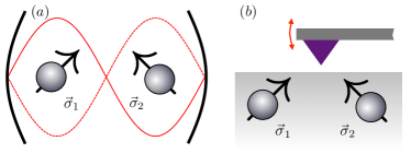
Figure 1: (color online). Schematic illustration for a generic spin-resonator system, comprising a set of spins $\left\{\vec{\sigma}_{i}\right\}$ coupled to a common resonator mode (as provided by e.g. (a) a transmission line or (b) nanomechanical oscillators), with a non-vanishing thermal occupation.

II The Scheme

We consider a set of spins (qubits) $i{=}1,2,\dots$ with transition frequencies $\omega_{q}$ coupled to a common (bosonic) cavity mode of frequency $\omega_{c}$, as described by the Hamiltonian $\left(\hbar{=}1\right)$

$$H=\omega_{c}a^{\dagger}a+\frac{\omega_{q}}{2}S^{z}+g\mathcal{S}\otimes\left(a+a^{\dagger}\right),$$ (1)

with $\mathcal{S}{=}\sum_{i,\alpha}\eta_{i}^{\alpha}\sigma_{i}^{\alpha},$ $S^{z}{=}\sum_{i}\sigma_{i}^{z}$, where $\vec{\sigma}_{i}$ refer to the usual Pauli matrices describing the qubits, and $a$ is the bosonic annihilation operator for the resonator mode. The operator $\mathcal{S}$ is a generalized (collective) spin operator which accounts for both transversal $\left(\alpha{=}x,y\right)$ and longitudinal $\left(\alpha{=}z\right)$ spin-resonator coupling; the unit-less parameters $\eta_{i}^{\alpha}$ capture potential anisotropies and inhomogeneities in the single-photon (or single-phonon) coupling constants $g_{i}^{\alpha}{=}\eta_{i}^{\alpha}g$. Similar to existing (low-temperature) schemes beaudoin16 ; taylor06 , the spin-resonator coupling $g{=}g(t)$ is assumed to be tunable on a timescale ${\ll}\omega^{-1}_{c}$; for details we refer to Appendix D.

Typically, for artificial atoms such as quantum dots the qubit transition frequencies $\omega_{q}$ are highly tunable. In what follows, we consider the regime where $\omega_{q}$ is much smaller than all other energy scales; therefore, for the purpose of our analytical derivation, effectively we take $\omega_{q}{=}0$. The robustness of our scheme against non-zero splittings $\left(\omega_{q}{>}0\right)$ will be discussed below. In this limit, the Hamiltonian given in Eq.(1) can be rewritten as

$$H=\omega_{c}\left(a+\frac{g}{\omega_{c}}\mathcal{S}\right)^{\dagger}\left(a+\frac{g}{\omega_{c}}\mathcal{S}\right)-\frac{g^{2}}{\omega_{c}}\mathcal{S}^{2}.$$ (2)

Using the relation $UaU^{\dagger}{=}a+\left(g/\omega_{c}\right)\mathcal{S},$ with the unitary (polaron) transformation $U{=}\exp\left[g/\omega_{c}\mathcal{S}\left(a-a^{\dagger}\right)\right]$, Eq.(2) can be recast into the form

$$H = U\underset{H_{0}}{\underbrace{\left[\omega_{c}a^{\dagger}a-\frac{g^{2}}{\omega_{c}}\mathcal{S}^{2}\right]}}U^{\dagger},$$ (3)

where we have used that $\mathcal{S}$ commutes with $U$. The time-evolution governed by the Hamiltonian $H$ reads

$$e^{-iHt}=e^{-iUH_{0}U^{\dagger}t} = Ue^{-i\omega_{c}ta^{\dagger}a}e^{i\frac{g^{2}}{\omega_{c}}t\mathcal{S}^{2}}U^{\dagger},$$ (4)

where the second equality directly follows from $\exp\left(x\right){=}\sum_{n}x^{n}/n!$ and $U^{\dagger}U{=}\mathds{1}$. For certain times where $\omega_{c}t_{m}{=}2\pi m$ (with $m$ integer), the first exponential equals the identity, $\exp\left[-i\omega_{c}ta^{\dagger}a\right]{=}\exp\left[-i2\pi ma^{\dagger}a\right]{=}\mathds{1}$, since the number operator $\hat{n}{=}a^{\dagger}a$ has an integer spectrum $0,1,2,\dots$. Thus, for $t_{m}{=}\left(2\pi/\omega_{c}\right)m$, the full time evolution reduces to

$$e^{-iHt_{m}}=e^{i\frac{g^{2}}{\omega_{c}}t_{m}\mathcal{S}^{2}}=\exp\left[i2\pi m\left(g/\omega_{c}\right)^{2}\mathcal{S}^{2}\right].$$ (5)

This relation comes with two major implications: (i) Our approach is not based on a perturbative argument; therefore, apart from Eq.(5), the resonator-mediated qubit-qubit interaction does not lead to any further undesired, spurious terms. (ii) Since the unitary transformation given in Eq.(5) does not contain any operators acting on the resonator mode, it is completely insensitive to the state of the resonator milburn99 ; soerensen00 ; soerensen99 , even though the spin-spin interactions present in $\mathcal{S}^{2}$ have been established effectively via the resonator degrees of freedom; similar considerations have been applied for the case of two (superconducting) qubits for a zero temperature mode royer16 and for small finite temperature $T$ in a classically modeled mode kerman13 . For specific times, the time-evolution in the polaron and the lab-frame fully coincide and become truly independent of the resonator mode, allowing for the realization of a thermally robust gate, without any need of cooling the resonator mode to the ground state. This statement holds provided that rethermalization of the resonator mode can be neglected over the relevant gate time. The experimental implications for this condition will be discussed below.

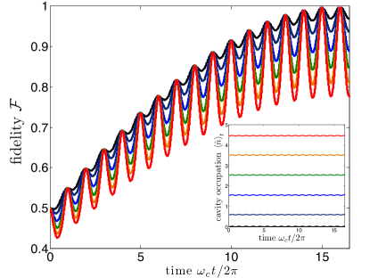
Figure 2: (color online). Fidelity $\mathcal{F}$ with the maximally entangled target state $\left|\Psi_{\mathrm{tar}}\right\rangle{=}\left(\left|\Uparrow\Downarrow\right\rangle+i\left|\Downarrow\Uparrow\right\rangle\right)/\sqrt{2}$ for transversal coupling $\left(\mathcal{S}{=}\sigma_{1}^{x}+\sigma_{2}^{x}\right)$, the initial product state $\rho\left(0\right){=}\left|\Uparrow\Downarrow\right\rangle\left\langle\Uparrow\Downarrow\right|\otimes\rho_{\mathrm{th}}\left(T\right)$ and different temperatures $k_{B}T/\omega_{c}{=}0,1,2,3,4,5$. Independently of the temperature $T$, the spins periodically disentangle from the (hot) resonator mode and systematically build-up entanglement among themselves. While the peaks are merely independent of temperature, the amplitude of the precursory oscillations do increase with temperature. Inset: Occupation of the resonator $\left\langle\hat{n}\right\rangle_{t}$ showing small oscillations due to weak entanglement between the qubits and the cavity mode soerensen00 . Other numerical parameters: $\omega_{q}/\omega_{c}{=}\Gamma=0$, $g/\omega_{c}{=}1/16$, $\kappa/\omega_{c}{=}Q^{-1}=10^{-5}$.

To further illustrate Eq.(5), let us consider three paradigmatic examples: (1) For longitudinal coupling ($\eta_{i}^{z}{=}1$, $\eta_{i}^{x}{=}\eta_{i}^{y}{=}0$), as could be realized (for example) with defect spins coupled to nanomechanical oscillators rabl10 , we can identify the effective spin-spin Hamiltonian $H_{\mathrm{eff}}{=}\Omega_{m}\left(\sigma_{1}^{z}+\sigma_{2}^{z}\right)^{2}$, which results in a relative phase $\phi{=}4\Omega_{m}$ for the states $\left|11\right\rangle{=}\left|\Uparrow\Uparrow\right\rangle,\left|00\right\rangle{=}\left|\Downarrow\Downarrow\right\rangle$ as compared to the states $\left|10\right\rangle$ and $\left|01\right\rangle$, respectively. By adding a local unitary on both qubits, such that $\left|0\right\rangle_{i}\rightarrow\exp\left(-i\phi/2\right)\left|0\right\rangle_{i}$ and $\left|1\right\rangle_{i}\rightarrow\exp\left(i\phi/2\right)\left|1\right\rangle_{i}$, in total for $\phi{=}\pi/2$ we obtain a controlled phase gate $U_{\mathrm{Cphase}}{=}\mathrm{diag}\left(1,1,1,-1\right),$ which gives a phase of $-1$ exclusively to $\left|11\right\rangle$, while leaving all other states invariant. Note that such a controlled phase gate can be implemented even in the presence of non-zero and inhomogeneous qubit level splittings $\left(\omega_{q}{>}0\right)$, when applying either fast local single qubit gates (to correct the effect of known $\omega_{q}{\neq}0$) or standard spin-echo techniques (to compensate unknown detunings), thereby lifting the requirement of having a small qubit level splitting $\omega_{q}$; see Appendix H for details. (2) Again for longitudinal coupling ($\eta_{i}^{z}{=}1$, $\eta_{i}^{x}{=}\eta_{i}^{y}=0$) and $N\geq 2$ qubits, Eq.(5) results in a unitary transformation $U{=}\exp\left[-i\theta I_{z}^{2}\right]$ generated by a non-linear top Hamiltonian describing precession around the $I_{z}{=}\sum_{i}\sigma_{i}^{z}$ axis with a rate depending on the $z$-component of angular momentum milburn99 , which can be used to simulate nonlinear spin models milburn99 . (3) For transversal coupling with $\mathcal{S}{=}\sigma_{1}^{x}+\sigma_{2}^{x},$ as could be realized (for example) with quantum dot based qubits embedded in circuit-QED cavities hu12 ; beaudoin16 or SAW cavities chen15 ; schuetz15 , we have $\mathcal{S}^{2}{=}2\times\mathds{1}+2\sigma_{1}^{x}\sigma_{2}^{x}$. Up to an irrelevant global phase $\phi_{\mathrm{gp}}$ due to the first term $\sim\mathds{1}$, we get

$$e^{-iHt_{m}}=e^{-i\phi_{\mathrm{gp}}}\underset{\equiv U_{\mathrm{id}}^{x}\left(m,g/\omega_{c}\right)}{\underbrace{\exp\left[i4\pi m\left(g/\omega_{c}\right)^{2}\sigma_{1}^{x}\sigma_{2}^{x}\right]}},$$ (6)

which for $m\left(g/\omega_{c}\right)^{2}{=}1/16$ yields a maximally entangling gate, that is $U_{\mathrm{id}}^{x}\left(1,1/4\right)\left|\Uparrow\Downarrow\right\rangle{=}\frac{1}{\sqrt{2}}\left(\left|\Uparrow\Downarrow\right\rangle+i\left|\Downarrow\Uparrow\right\rangle\right)$ etc., i.e., initial qubit product states evolve to maximally entangled states, irrespectively of the temperature of the resonator mode, on a timescale $t_{\mathrm{max}}{=}\pi/8g_{\mathrm{eff}}$ (where $g_{\mathrm{eff}}{=}g^{2}/\omega_{c}$); compare Fig.2 for an exemplary time evolution, starting initially from the product state $\rho\left(0\right){=}\left|\Uparrow\Downarrow\right\rangle\left\langle\Uparrow\Downarrow\right|\otimes\rho_{\mathrm{th}}\left(T\right)$, with the cavity mode in the thermal state $\rho_{\mathrm{th}}\left(T\right){=}Z^{-1}\exp\left[-\beta\omega_{c}a^{\dagger}a\right]$, and $\beta{=}1/k_{B}T$. Indeed entanglement peaks are observed at stroboscopic times $\left(\omega_{c}t_{m}{=}2\pi m\right)$, independent of the temperature $T$, culminating in a maximally entangled state at time $t_{\mathrm{max}}$.

III Coupling to the Environment

In the analysis above, we have ignored the presence of decoherence, which in any realistic setting will degrade the effects of coherent qubit-resonator interactions. Therefore, we complement our analytical findings with numerical simulations of the full master equation for the system’s density matrix $\rho$,

$$\dot{\rho} = -i\left[H,\rho\right]+\kappa\left(\bar{n}_{\mathrm{th}}+1\right)\mathcal{D}\left[a\right]\rho+\kappa\bar{n}_{\mathrm{th}}\mathcal{D}\left[a^{\dagger}\right]\rho$$ (7)

$$+\frac{\Gamma}{4}\sum_{i=1,2}\mathcal{D}\left[\sigma_{i}^{z}\right]\rho,$$

where the generic spin-resonator Hamiltonian $H$ is given in Eq.(1) and the last two dissipative terms in the first line of Eq.(7), with $\mathcal{D}\left[a\right]\rho{=}a\rho a^{\dagger}-\frac{1}{2}\left\{a^{\dagger}a,\rho\right\}$ and a cavity mode decay rate $\kappa{=}\omega_{c}/Q$, describe rethermalization of the cavity mode towards the thermal occupation $\bar{n}_{\mathrm{th}}{=}(\mathrm{exp}\left[\hbar\omega_{c}/k_{B}T\right]-1)^{-1}$ at temperature $T$; here, $Q$ is the quality-factor of the cavity. The last line in Eq.(7) describes dephasing of the qubits with a dephasing rate $\Gamma{\sim}1/T_{2}^{\star}$, where $T_{2}^{\star}$ is the time-ensemble-averaged dephasing time. As discussed in detail in Appendix J, the noise model underlying Eq.(7) is accurate in the experimentally most relevant regime of weak spin-resonator coupling $(g{\ll}\omega_{c})$, where (within the approximation of independent rates of variation cohen92 ) the interactions with the environment can be treated separately for spin and resonator degrees of freedom. In Eq.(7) we have ignored single spin relaxation processes, since the associated timescale $T_{1}$ is typically much longer than $T_{2}^{\star}$; still, relaxation processes could be included straightforwardly in our model by adding the decay terms $\dot{\rho}{=}\dots+T_{1}^{-1}\sum_{i}\mathcal{D}\left[\sigma_{i}^{-}\right]\rho$ and the corresponding error (infidelity) could be analyzed along the lines of our analysis shown below (see Appendix N for details).

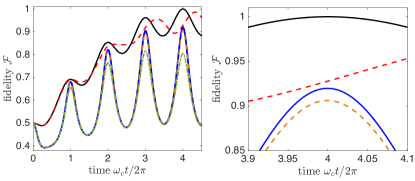
Figure 3: (color online). Fidelity $\mathcal{F}$ (left) in the presence of noise, with a zoom-in around $t_{\mathrm{max}}$ (right). As a benchmark, the solid (topmost) black line refers to the quasi-ideal limit ($\Gamma=0$, $\kappa/\omega_{c}{=}Q^{-1}=10^{-5}$ and $k_{B}T/\omega_{c}{=}0$), while (only) the red dashed curve accounts for a non-zero qubit level splitting $\omega_{q}/\omega_{c}{=}0.1$. The solid blue line also accounts for dephasing of the qubits with a (rather large) dephasing rate $\Gamma/\omega_{c}{=}1\%$ and finite thermal occupation of the resonator mode with $k_{B}T/\omega_{c}{=}5$ ($\bar{n}_{\mathrm{th}}{\approx}4.5$). The results are relatively insensitive to the quality factor of the cavity, provided that $\kappa_{\mathrm{eff}}{\ll}\Gamma$; the orange dashed line (where $Q{=}10^{3}$) is basically identical to the $Q{=}10^{5}$ scenario, whereas the green dash-dotted (lowest) one with $Q{=}10^{2}$ (that is, $\kappa/\omega_{c}{=}\Gamma/\omega_{c}{=}1\%$) shows a clear reduction in $\mathcal{F}$. This result can be traced back to the hot-gate requirement given in Eq.(8). Ideally, maximum entanglement is reached for $f_{c}t{=}4$, with several precursory oscillation peaks at $f_{c}t{=}1,2,3$. Other numerical parameters: $g/\omega_{c}{=}1/8$, $\omega_{q}/\omega_{c}{=}0$ (except for the red dashed curve where $\omega_{q}/\omega_{c}{=}0.1$).

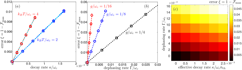
Figure 4: (color online). Errors ($\xi{=}1-\mathcal{F}_{\mathrm{max}}$) due to rethermalization of the cavity mode (a) and qubit dephasing (b). (a) Rethermalization-induced error for $k_{B}T/\omega_{c}{=}2$ (blue) and $k_{B}T/\omega_{c}{=}4$ (red), and $\Gamma{=}0$. The error $\xi_{\kappa}$ is found to be independent of $\mu{=}g/\omega_{c}$: $\mu{=}1/16$ (squares) and $\mu{=}1/8$ (blue circles and red diamonds). (b) Dephasing induced errors for $\mu{=}1/4$ (squares), $\mu{=}1/8$ (circles) and $\mu{=}1/16$ (diamonds); here, $\kappa/\omega_{c}{=}10^{-6}$ and $k_{B}T/\omega_{c}{=}0.01$. In both cases the linear error scaling is verified. Other numerical parameters: $\omega_{q}/\omega_{c}{=}0$. (c) Total error $\xi$ as a function of both the effective rethermalization rate ${\sim}\kappa/\omega_{c}\bar{n}_{\mathrm{th}}{\sim}\bar{n}_{\mathrm{th}}/Q$ and the spin dephasing rate ${\sim}\Gamma/\omega_{c}$ for $g/\omega_{c}{=}1/16$, $k_{B}T/\omega_{c}{=}2$ and $\omega_{q}{=}0$.

Numerical results.—To quantitatively capture the effects of decoherence, in the following we provide numerical results of the Master equation Eq.(7), for the initial product state $\rho\left(0\right){=}\left|\Uparrow\Downarrow\right\rangle\left\langle\Uparrow\Downarrow\right|\otimes\rho_{\mathrm{th}}\left(T\right)$, and (transversal) spin-resonator coupling with $\eta_{i}^{x}{=}1$ and $\eta_{i}^{y}{=}\eta_{i}^{z}=0$. As a figure of merit for our protocol, we quantify the state fidelity $\mathcal{F}{=}\left<\Psi_{\mathrm{tar}}|\varrho|\Psi_{\mathrm{tar}}\right>$ with the maximally entangled target state $\left|\Psi_{\mathrm{tar}}\right\rangle{=}\left(\left|\Uparrow\Downarrow\right\rangle+i\left|\Downarrow\Uparrow\right\rangle\right)/\sqrt{2}$; here, $\varrho{=}\mathrm{tr}_{a}\left[\rho\right]$ refers to the density matrix of the qubits, with $\mathrm{tr}_{a}\left[\dots\right]$ denoting the trace over the resonator degrees of freedom. As shown in Appendix O, similar results can be obtained for the average gate fidelity. Typical results from our numerical simulations in the presence of noise are displayed in Fig.3. As expected from our analytical results, for $\omega_{c}t_{m}{=}2\pi m$ the two qubits disentangle from the thermally populated resonator mode and systematically evolve towards the maximally entangled target state $\left|\Psi_{\mathrm{tar}}\right\rangle$; for example, for $g/\omega_{c}{=}1/8$ (as used in Fig.3), the spins evolve towards $U_{\mathrm{id}}^{x}\left(1,1/8\right)\left|\Uparrow\Downarrow\right\rangle{=}\cos\left(\pi/16\right)\left|\Uparrow\Downarrow\right\rangle+i\sin\left(\pi/16\right)\left|\Downarrow\Uparrow\right\rangle$ for $m{=}1$, $U_{\mathrm{id}}^{x}\left(2,1/8\right)\left|\Uparrow\Downarrow\right\rangle{=}\cos\left(\pi/8\right)\left|\Uparrow\Downarrow\right\rangle+i\sin\left(\pi/8\right)\left|\Downarrow\Uparrow\right\rangle$ for $m{=}2$, and $U_{\mathrm{id}}^{x}\left(3,1/8\right)\left|\Uparrow\Downarrow\right\rangle{=}\cos\left(3\pi/16\right)\left|\Uparrow\Downarrow\right\rangle+i\sin\left(3\pi/16\right)\left|\Downarrow\Uparrow\right\rangle$ for $m{=}3$, before the entanglement build-up culminates in the fully-entangling dynamics $U_{\mathrm{id}}^{x}\left(4,1/8\right)\left|\Uparrow\Downarrow\right\rangle{=}\left(\left|\Uparrow\Downarrow\right\rangle+i\left|\Downarrow\Uparrow\right\rangle\right)/\sqrt{2}$. For all practical purposes, this statement holds independently of the temperature $T$ and the associated thermal occupation of the resonator mode $\bar{n}_{\mathrm{th}}{\approx}k_{B}T/\hbar\omega_{c}$, provided that the quality factor of the cavity $Q$ is sufficiently high; a quantitative statement specifying this regime will be given below. Moreover, while our analytical treatment has assumed $\omega_{q}{=}0$, we have numerically verified that the proposed protocol is robust against non-zero level splittings of the qubits $\omega_{q}/\omega_{c}{\lesssim}0.1$; compare the dashed line in Fig.3 and further information provided in Appendices G, H and K.

IV Gate time requirements: Error scaling

As described by Eq.(7), coupling to the environment leads to two dominant error sources: (i) rethermalization of the resonator mode with an effective rate ${\sim}\kappa\bar{n}_{\mathrm{th}}$, and (ii) dephasing of the qubits on a timescale ${\sim}T_{2}^{\star}$. For any hot gate, the associated gate time $t_{\mathrm{gate}}{\sim}g_{\mathrm{eff}}^{-1}$, with $g_{\mathrm{eff}}{=}g^{2}/\omega_{c}{=}\mu^{2}\omega_{c}$, has to be shorter than the time-scale associated with the effective (thermally-enhanced) rethermalization rate $\kappa_{\mathrm{eff}}{=}\kappa\bar{n}_{\mathrm{th}}{\approx}k_{B}T/Q$. For the gate described above, this directly leads to the requirement

$$g^{2}/\omega_{c}\gg k_{B}T/Q\,\,\,\,\,\Leftrightarrow\,\,\,\,\,k_{B}T\ll Q\mu^{2}\omega_{c}.$$ (8)

Thus, for $T{=}1\mathrm{K}$ $\left(k_{B}T/2\pi{\approx}20\mathrm{GHz}\right)$ and a cavity quality factor $Q{\approx}10^{5}-10^{6}$, we need $g_{\mathrm{eff}}/2\pi{\gg}\left(20-200\right)\mathrm{kHz}$. Provided that our assumption $\omega_{c}{\gg}\omega_{q}$ is still fulfilled, for fixed temperature $T$, quality factor $Q$ and coupling $g$, relation (8) may be conveniently fulfilled by choosing $\omega_{c}$ sufficiently small, up to the lower limit $\omega_{c}{\geq}4g$ (which is needed to fulfill $m{\geq}1$; compare Appendix C) and at the cost of a potentially relatively large device (since the device dimensions scale with ${\sim}\lambda_{c}{\sim}\omega_{c}^{-1}$). Conversely, for fixed $\mu{=}g/\omega_{c}$ taylor06 ; chen15 ; schoelkopf08 , Eq.(8) can be achieved by choosing $\omega_{c}$ sufficiently large. In addition, the gate time has to be short compared to the qubit’s dephasing time $T_{2}^{\star}{\sim}\Gamma^{-1}$, which gives the second requirement

$$g^{2}/\omega_{c}\gg\Gamma\,\,\,\,\,\Leftrightarrow\,\,\,\,\,\Gamma\ll\mu^{2}\omega_{c}.$$ (9)

For concreteness, let us consider a specific setup where conditions (8) and (9) can be met with state-of-the-art technology: Quantum dots (QDs) have been successfully integrated with superconducting microwave cavities, with a relatively large charge-cavity coupling of $g_{\mathrm{ch}}/2\pi{\sim}\left(20-100\right)\mathrm{MHz}$ liu14 ; frey12 ; petersson12 ; viennot14 ; toida13 . For QD spin qubits a vacuum Rabi frequency of $g_{\mathrm{sp}}/2\pi{\sim}1\mathrm{MHz}$ has been predicted hu12 ; petersson12 ; jin12 , with the potential to increase this coupling to $\sim 10\mathrm{MHz}$ with new, recently demonstrated cavity designs samkharadze15 . Furthermore, for superconducting transmission line resonators quality factors $Q{\sim}10^{6}$ have been demonstrated barends08 . Then, taking $g_{\mathrm{sp}}/2\pi{=}10\mathrm{MHz}$, $\omega_{c}/2\pi{\approx}(0.16-1)\mathrm{GHz}$, i.e., $g_{\mathrm{eff}}/2\pi{\approx}(0.1-0.6)\mathrm{MHz}$, and $Q{=}10^{6}$, conditions (8) and (9) can be met simultaneously for temperatures $T{\sim}1\mathrm{K}$ [since $T{\ll}5(30)\mathrm{K}$ to fulfill condition (8) for $g_{\mathrm{eff}}/2\pi{\approx}0.1(0.6)\mathrm{MHz}$] and dephasing timescales $T_{2}^{\star}{\sim}100\mu\mathrm{s}$ [since $\Gamma/2\pi{\ll}\left(0.1-0.6\right)\mathrm{MHz}$ to fulfill condition (9)], as has been demonstrated with isotopically purified Si samples veldhorst14 . Therefore, a faithful implementation of our gate will not require cooling to milli-Kelvin temperatures. Similar promising estimates also apply to spin-qubits coupled to SAW-resonators; compare Appendix I.

In the following, we quantify the infidelities induced by the two error sources outlined above: Rethermalization of the resonator mode during the gate leads to errors (infidelities) if the resonator is entangled with the qubits. Due to leakage of which-way information, resonator noise leads to qubit dephasing at a rate proportional to the relevant separation in phase space, that is the square of the resonator displacement $\mu{=}g/\omega_{c}$ rabl10 . The effective rethermalization-induced dephasing rate for the qubits is then $\Gamma_{\mathrm{eff}}{\sim}\kappa\bar{n}_{\mathrm{th}}\left(g/\omega_{c}\right)^{2}$. To obtain a simple estimate for the rethermalization-induced error, this effective rate $\Gamma_{\mathrm{eff}}$ is multiplied with the relevant gate time which scales as $t_{\mathrm{gate}}{\sim}\omega_{c}/g^{2}$, yielding the error $\xi_{\kappa}{\sim}\left(\kappa/\omega_{c}\right)\bar{n}_{\mathrm{th}}$, which is independent of the spin-resonator coupling strength $g$ royer16 ; rabl10 ; for a full analytical derivation we refer to Appendix L. However, since the overall gate time $t_{\mathrm{gate}}{\sim}\omega_{c}/g^{2}$ increases for small $\mu{=}g/\omega_{c}$, errors will accumulate due to direct qubit decoherence processes. Accordingly, errors due to qubit dephasing are expected to scale as $\xi_{\Gamma}{\sim}\Gamma/g_{\mathrm{eff}}{\sim}\mu^{-2}\Gamma/\omega_{c}.$ This simple linear scaling holds for a Markovian noise model where qubit dephasing is described by a standard pure dephasing term [compare Eq.(7)] leading to an exponential loss of coherence $\sim\exp\left[-t/T_{2}^{\star}\right]$; for non-Markovian qubit dephasing a better, sub-linear scaling can be expected schuetz15 ; rabl10 . For small infidelities $\left(g_{\mathrm{eff}}{\gg}\kappa_{\mathrm{eff}},\Gamma\right)$, the individual linear error terms due to cavity rethermalization and qubit dephasing can be added independently, yielding the total error

$$\xi\approx\alpha_{\kappa}\left(\kappa/\omega_{c}\right)\bar{n}_{\mathrm{th}}+\alpha_{\Gamma}\Gamma/\omega_{c}.$$ (10)

This simple linear error model has been verified numerically; compare Fig.4. Based on these results we extract the coefficients $\alpha_{\kappa}{\approx}4$ (which is approximately independent of $g$ royer16 ; compare Appendices K and L for details) and $\alpha_{\Gamma}{\approx}0.1/\mu^{2}$. For $g_{\mathrm{sp}}/2\pi{\approx}10\mathrm{MHz}$ samkharadze15 ; hu12 ; jin12 , a relatively low resonator frequency $\omega_{c}/2\pi{=}16g_{\mathrm{sp}}/2\pi{=}160\mathrm{MHz}$, $T{=}1\mathrm{K}$ (corresponding to $\bar{n}_{\mathrm{th}}{\approx}130$), $Q{=}10^{5}$ samkharadze15 ; barends08 and a realistic dephasing rate $\Gamma/2\pi{\approx}0.1\mathrm{MHz}$ veldhorst14 , that is $\kappa/\omega_{c}\bar{n}_{\mathrm{th}}{\approx}1.3\times 10^{-3}$ and $\Gamma/\omega_{c}{\approx}6\times 10^{-4}$, our estimates then predict an overall infidelity of $\xi{\approx}2\%$, with the potential to reach error rates $\xi{\approx}0.2\%$ below the threshold for quantum error correction for state-of-the-art experimental parameters ($Q{\approx}10^{6}$, $\Gamma/2\pi{\approx}10\mathrm{kHz}$) knill05 ; veldhorst14 ; barends08 . This simple estimate compares well with other bus-based, two-qubit (hot) gates reaching fidelities ${\sim}97\%$ kirchmair09 ; rabl10 ; chow12 and has been corroborated by numerical simulations that fully account for higher-order errors; compare the density plot in Fig.4(c). We like to emphasize that, due to the fundamental temperature-insensitivity of our gate, technological improvements in the achievable $Q$-factor directly translate to a proportional reduction of thermalization-induced errors and therefore increase the acceptable temperature. Note that the error estimate given in Eq.(10) assumes perfect timing of the gate, as the maximum fidelity is reached exactly at time $t_{\mathrm{max}}$, whereas under experimentally realistic conditions there will be a residual error due to imperfect timing of the gate. However, as shown in Appendix K, for sufficiently small, but realistic timing accuracies of $\left(\omega_{c}/2\pi\right)\Delta t{\lesssim}1\%$ and small spin-resonator coupling $g/\omega_{c}{\lesssim}1/16$ (implying small oscillation amplitudes), the effects of time-jitter become negligible.

V Conclusions & Outlook

To conclude, we have proposed and analyzed a high-fidelity hot gate for generic spin-resonator systems which allows for coherent spin-spin coupling, even in the presence of a thermally populated resonator mode. While we have mostly focused on just two spins, our scheme fully applies to more than two spins, which should allow for the preparation of maximally entangled multi-partite states; as shown in Ref.moelmer99 in the context of trapped ions, a propagator of the form given in Eq.(5) applied to the initial product state $\left|00\cdots 0\right\rangle$ may be used to generate states of the form $1/\sqrt{2}\left(\left|00\cdots 0\right\rangle+e^{i\phi}\left|11\cdots 1\right\rangle\right)$, where $\left|00\cdots 0\right\rangle$ and $\left|11\cdots 1\right\rangle$ are product states with all qubits in the same state $\left|0\right\rangle$ or $\left|1\right\rangle$, respectively.

Appendices

The following Appendices provide additional background material to specific topics of the main text. They are structured as follows: In Sec.A we provide typical thermal occupation numbers $\bar{n}_{\mathrm{th}}$ for relevant experimental parameter regimes. In Sec.B we compare the ideal evolution in the lab frame to the one in the polaron frame. In Sec.C we derive the ideal gate time $t_{\mathrm{max}}$. In Sec.D we discuss a prototypical implementation of a spin-resonator system that allows for time-dependent control of the spin-resonator $g=g\left(t\right)$, as required for the faithful realization of the proposed hot gate. In Sec.E we discuss the standard approach to coupling spins via a common resonator mode in the dispersive regime, in which, in contrast to the proposed hot gate, the spin degrees of freedom do not fully disentangle from the resonator mode. In Sec.F we compare our general result to a perturbative calculation in the framework of a Schrieffer-Wolff transformation. In Secs.G and H we analyze in detail the effects coming from a non-zero qubit level splitting ($\omega_{q}/\omega_{c}>0$). In Sec.I we provide further details on how to implement experimental candidate systems governed by the class of Hamiltonians given in Eq.(1), using quantum dots embedded in high-quality surface acoustic wave (SAW) resonators. In Sec.J we provide a microscopic derivation of the Master equation given in Eq.(7) of our manuscript. In Sec.K we present further results based on the numerical simulation of the master equation given in Eq.(7) of the main text. In Sec.L we derive an analytical expression for rethermalization-induced errors, while Sec.M provides an analytical model for dephasing-induced errors. In Sec.N we address in detail errors induced by relaxation processes. In Sec.O we conclude with a discussion on the average gate fidelity.

Appendix A Thermal Occupation

Here, we first provide typical thermal occupation numbers $\bar{n}_{\mathrm{th}}$ for relevant experimental parameter regimes. At a temperature $T=4\mathrm{K}$, a (mechanical) oscillator of frequency $\omega_{c}/2\pi\sim\left(1-10\right)\mathrm{GHz}$ has an thermal equilibrium occupation number much larger than one, $\bar{n}_{\mathrm{th}}\approx 8-80$: compare Fig.5.

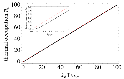
Figure 5: (color online). Thermal occupation $\bar{n}_{\mathrm{th}}=(\mathrm{exp}\left[\hbar\omega_{c}/k_{B}T\right]-1)^{-1}$ (black solid line) and high-temperature approximate result $\bar{n}_{\mathrm{th}}\approx k_{B}T/\hbar\omega_{c}$ (red dashed line). For $T=4\mathrm{K}$ and $\omega_{c}/2\pi=1\mathrm{GHz}$ ($\omega_{c}/2\pi=10\mathrm{GHz}$), we have $k_{B}T/\hbar\omega_{c}\approx 80$ ($k_{B}T/\hbar\omega_{c}\approx 8$). For $T=1\mathrm{K}$ and $\omega_{c}/2\pi=1\mathrm{GHz}$ ($\omega_{c}/2\pi=10\mathrm{GHz}$), we have $\bar{n}_{\mathrm{th}}\approx 20$ ($\bar{n}_{\mathrm{th}}\approx 2$).

Appendix B Polaron vs. Lab Frame

In this Appendix we show that for stroboscopic times the ideal time evolution in the lab frame fully coincides with the one in the polaron frame.

In the ideal (noise-free) scenario, the evolution of the system in the lab frame, comprising both spin and resonator degrees of freedom, is described by Schrödinger’s equation

$$i\frac{d}{dt}\left|\psi\right\rangle_{t}=H\left|\psi\right\rangle_{t}.$$ (11)

In the polaron frame, the time evolution is governed by

$$i\frac{d}{dt}\tilde{\left|\psi\right\rangle}_{t}=H_{0}\tilde{\left|\psi\right\rangle}_{t},$$ (12)

where $\tilde{\left|\psi\right\rangle}_{t}=U^{\dagger}\left|\psi\right\rangle_{t}$, $U=\exp\left[\mu S\left(a-a^{\dagger}\right)\right]$, and $H_{0}=U^{\dagger}HU=\omega_{c}a^{\dagger}a-\frac{g^{2}}{\omega_{c}}\mathcal{S}^{2}$; the polaron transformation $U$ entangles spin with resonator degrees of freedom. The solution to Eq.(12) reads $\tilde{\left|\psi\right\rangle}_{t}=\exp\left[-iH_{0}t\right]\tilde{\left|\psi\right\rangle}_{0}$. Using the relation $\exp\left[-i\omega_{c}ta^{\dagger}a\right]=\exp\left[-i2\pi ma^{\dagger}a\right]=\mathds{1}$ for stroboscopic times ($\omega_{c}t_{m}=2\pi m$, with $m$ integer), full time evolution in the polaron frame reduces to

$$\tilde{\left|\psi\right\rangle}_{t_{m}}=e^{i2\pi m\mu^{2}\mathcal{S}^{2}}\tilde{\left|\psi\right\rangle}_{0}.$$ (13)

Transforming back to the lab frame with $\tilde{\left|\psi\right\rangle}_{t}=U^{\dagger}\left|\psi\right\rangle_{t}$, and using that $U$ commutes with the propagator $\exp\left[i2\pi m\mu^{2}\mathcal{S}^{2}\right]$, we obtain the (stroboscopic) solution in the lab frame, $\left|\psi\right\rangle_{t_{m}}=e^{i2\pi m\mu^{2}\mathcal{S}^{2}}\left|\psi\right\rangle_{0}$, which fully coincides with the one in the polaron frame.

Appendix C Gate Time

Ideally, the gate time $t_{\mathrm{gate}}$ has to fulfill two conditions: (i) it has to be chosen stroboscopically, that is $\omega_{c}t_{\mathrm{gate}}=2\pi m$, with $m=1,2,\dots$ with (ii) the parameters such that $m\mu^{2}=1/16$ in order to obtain a maximally-entangling gate (in the absence of noise). Combination of (i) and (ii) then yields the ideal gate time

$$t_{\mathrm{max}}=\frac{\pi}{8g_{\mathrm{eff}}},$$ (14)

as given in the main text. The gate time $t_{\mathrm{max}}$ should be short compared to the relevant noise timescales, which yields the requirement $g_{\mathrm{eff}}\gg\kappa_{\mathrm{eff}},\Gamma$. In principle, large values of $g_{\mathrm{eff}}=g^{2}/\omega_{c}$ can be obtained by choosing the resonator frequency $\omega_{c}$ sufficiently small, provided that $\omega_{c}$ can be tuned independently of $g$. This can be done up to the lower bound $\omega_{c}\geq 4g$ which follows directly from the requirement $m=1/\left(16\mu^{2}\right)\geq 1$.

Appendix D Time-dependent Control of the Spin-Resonator Coupling

In this Appendix we discuss in detail a prototypical implementation of a spin-resonator system that allows for time-dependent control of the spin-resonator coupling $g=g\left(t\right)$, as required for the faithful realization of the proposed hot gate. Here, we first focus on a charge qubit embedded in a lithographically defined double quantum dot (DQD) containing a single electron, and then extend our analysis to a singlet-triplet spin qubit made out two electrons in such a DQD. Based on the electric dipole interaction, this type of device may be coupled either to a microwave transmission line resonator in a circuit-QED-like setup, as investigated theoretically and experimentally in (for example) Refs.frey12 ; petersson12 ; viennot14 , or a surface-acoustic-wave resonator, as described in Refs.schuetz15 ; chen15 . Our approach then employs standard all-electrical manipulation strategies, in which external, tunable gate voltages are used for (basically) in-situ control of the effective spin-resonator coupling childress04 , provided that standard adiabaticity conditions are fulfilled beaudoin16 , with the additional requirement of having a relatively small qubit transition frequency $\omega_{q}$ when the (hot) gate is turned on; as shown in Sec.H, this condition can be dropped, however, for longitudinal spin-resonator coupling.

D.1 Double Quantum Dot Charge Qubit

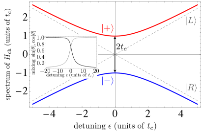
Figure 6: (color online). Spectrum of the DQD Hamiltonian in the single-electron regime, $H_{\mathrm{ch}}=\frac{\epsilon}{2}\tau^{z}+t_{c}\tau^{x}$, as a function of the interdot detuning parameter $\epsilon$. Inset: Mixing parameters $\sin\theta$ (black solid) and $\cos\theta$ (gray dashed) as a function of the interdot detuning parameter $\epsilon$.

The Hamiltonian describing a tunnel-coupled DQD in the single-electron regime coupled to a cavity of frequency $\omega_{c}$ is given by jin11 ; kulkarni14 ; gullans15

$$H=\frac{\epsilon}{2}\tau^{z}+t_{c}\tau^{x}+\omega_{c}a^{\dagger}a+g_{\mathrm{ch}}\tau^{z}\otimes\left(a+a^{\dagger}\right),$$ (15)

where $\epsilon$ is the (tunable) level detuning between the dots, $t_{c}$ gives the (tunable) tunnel coupling, and $g_{\mathrm{ch}}$ refers to the single photon (phonon) coupling strength between the resonator and the DQD. The electron charge state is described in terms of orbital Pauli operators defined as $\tau^{z}=\left|L\right\rangle\left\langle L\right|-\left|R\right\rangle\left\langle R\right|$ and $\tau^{x}=\left|L\right\rangle\left\langle R\right|+\left|R\right\rangle\left\langle L\right|$, respectively, with $\left|L\right\rangle\left(\left|R\right\rangle\right)$ corresponding to the state where the electron is localized in the left (right) dot, while $a^{\dagger}\left(a\right)$ are the standard resonator creation (annihilation) operators.

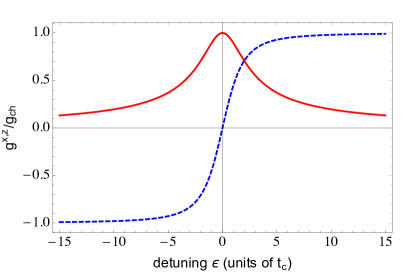
Figure 7: (color online). Effective spin-resonator coupling $g^{x}$ (solid) and $g^{z}$ (dashed) as a function of the interdot detuning parameter $\epsilon$.

Diagonalization of the first two terms in the Hamiltonian $H$, that is $H_{\mathrm{ch}}=\frac{\epsilon}{2}\tau^{z}+t_{c}\tau^{x}$, yields the electronic charge eigenstates

$$\left|+\right\rangle = \cos\theta\left|L\right\rangle+\sin\theta\left|R\right\rangle,$$ (16)

$$\left|-\right\rangle = -\sin\theta\left|L\right\rangle+\cos\theta\left|R\right\rangle,$$ (17)

where the mixing angle is given by $\tan\theta=2t_{c}/\left(\epsilon+\omega_{q}\right)$, and $\omega_{q}=\sqrt{\epsilon^{2}+4t_{c}^{2}}$ refers to the energy splitting between the eigenstates $\left|\pm\right\rangle$; compare Fig.6. The logical qubit basis is (by definition) given by the superposition states $\left|\pm\right\rangle=\left(\left|L\right\rangle\pm\left|R\right\rangle\right)/\sqrt{2}$ at the charge degeneracy point $\left(\epsilon=0\right)$, where to first order the qubit is insensitive to charge fluctuations $\left(d\omega_{q}/d\epsilon=0\right)$. In the eigenbasis of $H_{\mathrm{ch}}$, and after a simple gauge transformation $\left(a\rightarrow-a,a^{\dagger}\rightarrow-a^{\dagger}\right)$, the spin-resonator Hamiltonian given in Eq.(15) can be rewritten as

$$H = \frac{\omega_{q}}{2}\sigma^{z}+\omega_{c}a^{\dagger}a+\left(g^{x}\sigma^{x}-g^{z}\sigma^{z}\right)\otimes\left(a+a^{\dagger}\right).$$ (18)

Here, we have introduced the Pauli operators as $\sigma^{z}=\left(\left|+\right\rangle\left\langle+\right|-\left|-\right\rangle\left\langle-\right|\right)$, and $\sigma^{x}=\left(\left|+\right\rangle\left\langle-\right|+\left|-\right\rangle\left\langle+\right|\right)$; the transversal and longitudinal coupling parameters are given by

$$g^{x} = g_{\mathrm{ch}}\frac{2t_{c}}{\omega_{q}},$$ (19)

$$g^{z} = g_{\mathrm{ch}}\frac{\epsilon}{\omega_{q}}.$$ (20)

By redefining the interdot detuning parameter as $\epsilon\rightarrow-\epsilon$ (or, equivalently by relabeling $\left|L\right\rangle\leftrightarrow\left|R\right\rangle$), the spin-resonator Hamiltonian $H$ may be expressed as childress04 ; gullans15

$$H=\frac{\omega_{q}}{2}\sigma^{z}+\omega_{c}a^{\dagger}a+\left(g^{x}\sigma^{x}+g^{z}\sigma^{z}\right)\otimes\left(a+a^{\dagger}\right).$$ (21)

Both, the effective transversal coupling parameter $g^{x}$ as well as the longitudinal coupling parameter $g^{z}$ can be controlled via rapid all-electrical tuning of either the interdot detuning parameter $\epsilon$ and/or the tunnel splitting $t_{c}$ (recall $\omega_{q}=\sqrt{\epsilon^{2}+4t_{c}^{2}}$) beaudoin16 ; childress04 ; frey12 ; gullans15 ; kulkarni14 ; trif08 . As shown in Fig.7, the transversal coupling parameter $g^{x}$ is maximized around $\epsilon=0$ (that is, when the electron is delocalized in both dots), while it is strongly suppressed for $\left|\epsilon\right|\gg t_{c}$. Conversely, the longitudinal coupling parameter $g^{z}$ is maximized for $\left|\epsilon\right|\gg t_{c}$, while it is strongly suppressed for small detuning $\left|\epsilon\right|\ll t_{c}$. Note that, outside of our regime of interest, in the limit where $\delta,g_{\mathrm{ch}}\ll\omega_{c}$ (with $\delta=\omega_{q}-\omega_{c}$) one can perform a rotating-wave approximation yielding the standard Jaynes-Cummings Hamiltonian, as widely discussed in the literature (see e.g. Refs.frey12 ; trif08 ; schuetz15 ; childress04 ; jin11 ; kulkarni14 ).

Then, since the parameters $\epsilon\left(t\right)$ and $t_{c}\left(t\right)$ can be tuned all-electrically on very fast timescales, the protocol for the proposed hot gate proceeds as follows: (i) For $\epsilon\sim 0$, the hot gate is turned on, with $g^{x}\approx g_{\mathrm{ch}}$ and $g^{z}\sim 0$ (corresponding to purely transversal spin-resonator coupling as discussed extensively in the main text). In this regime, the qubit level splitting is set by the (highly tunable) tunnel-coupling, according to $\omega_{q}\approx 2t_{c}$, which should be chosen to be much smaller than the cavity frequency $\left(t_{c}\ll\omega_{c}\right)$ in order to satisfy the requirements of the proposed hot gate. (ii) After some well-controlled (stroboscopic) time $t_{m}=2\pi m/\omega_{c}$, the hot gate can be turned off by sweeping $\epsilon$ to large detuning values $\epsilon\gg t_{c}$.

Both regimes are readily achievable in the quantum dot setting: Due to the exponential dependence of tunnel coupling strength $t_{c}$ on gate voltage, the interdot barrier characterized by $t_{c}$ can be varied from about $100\mu\mathrm{eV}$ (verified by the broadening of the time-averaged charge transition; note that for much larger tunnel couplings, two neighboring dots become one single dot) all the way down to less than $10^{-12}\mathrm{eV}\sim 10^{-6}\mathrm{GHz}$ (corresponding to a millisecond timescale, as verified by real-time detection of single charges hopping on or off the dot) hanson07-sm , which is five to six orders of magnitude smaller than realistic cavity frequencies. Similarly, the detuning $\epsilon$ between the dots can be varied anywhere between zero and a positive or negative detuning equal to the addition energy, at which point additional electrons are pulled into the dot. The typical energy scale for the addition energy is very large $\left(\sim 1-3\mathrm{meV}\right)$ hanson07-sm .

Note that in the proposed off-setting [step (ii)] the qubits and the cavity are not strictly decoupled due to the non-vanishing longitudinal term (compare Fig.7). For $g_{\mathrm{ch}}\ll\omega_{c}$, this coupling is usually neglected within a rotating-wave approximation childress04 ; frey12 ; jin11 . However, here we provide an exact treatment, that takes into account the energy shifts and couplings arising from the (fast rotating) qubit-cavity coupling term. For $g^{x}=0$, the Hamiltonian $H$ can be diagonalized exactly, yielding the eigenstates $\left|\sigma\right\rangle\otimes D^{\dagger}(\sigma\frac{g^{z}}{\omega_{c}})\left|n\right\rangle$ with the corresponding eigenenergies $\epsilon\left(\sigma,n\right)=\sigma\omega_{q}/2-g_{z}^{2}/\omega_{c}+n\omega_{c}$, with $\sigma=\pm$ for spin-up and spin-down, respectively, the displacement operator $D\left(\alpha\right)=\exp\left[\alpha a^{\dagger}-\alpha^{*}a\right]$ and $\left|n\right\rangle$ denoting the usual Fock states. This treatment can be extended straightforwardly to more than one qubit.

While the analysis above has focused on a single charge qubit, in the following we consider two qubits of this type, coupled to a common resonator mode. Then, for two qubits and purely longitudinal spin-resonator coupling, in the presence of a non-zero (and potentially large, $\omega_{q}\sim\left|\epsilon\right|$) level splitting $\omega_{q}$ the time-evolution generated by the Hamiltonian $H$ reads

$$U\left(t_{m}\right)=e^{-iHt_{m}}=e^{-i\frac{\omega_{q}}{2}S^{z}t_{m}}U_{\mathrm{id}}^{z}\left(t_{m}\right),$$ (22)

with the ideal evolution $U_{\mathrm{id}}^{z}\left(t_{m}\right)=\exp\left[i4\pi m\mu^{2}\sigma_{1}^{z}\sigma_{2}^{z}\right]$, up to an irrelevant global phase. Therefore, in the regime $\left|\epsilon\right|\gg t_{c}$, a general two-qubit state $\left|\Psi_{2q}\right\rangle=c_{00}\left|\Downarrow\Downarrow\right\rangle+c_{01}\left|\Downarrow\Uparrow\right\rangle+c_{10}\left|\Uparrow\Downarrow\right\rangle+c_{11}\left|\Uparrow\Uparrow\right\rangle$ evolves as

$$U\left(t_{m}\right)\left|\Psi_{2q}\right\rangle = e^{+2im\pi\frac{\omega_{q}}{\omega_{c}}}c_{00}\left|\Downarrow\Downarrow\right\rangle+e^{-2im\pi\frac{\omega_{q}}{\omega_{c}}}c_{11}\left|\Uparrow\Uparrow\right\rangle$$ (23)

$$+e^{-8im\pi\mu^{2}}\left(c_{01}\left|\Downarrow\Uparrow\right\rangle+c_{10}\left|\Uparrow\Downarrow\right\rangle\right)$$

When tuning the qubit level splitting on resonance $\left(\omega_{q}\approx\left|\epsilon\right|=\omega_{c}\right)$, such that $\exp\left[\pm 2im\pi\omega_{q}/\omega_{c}\right]=1$ for all $m=1,2,3\dots$, for certain times $t^{\star}=2\pi m^{\star}/\omega_{c}=\pi/2g_{\mathrm{eff}}$, this unitary returns the original state, since $U_{\mathrm{id}}^{z}\left(t^{\star}\right)=\mathds{1}$, and therefore, absent any other noise sources, leaves the (typically entangled) state prepared by the first step (i) with $g^{x}=g_{\mathrm{ch}}$, $g^{z}=0$ unaffected; recall that $\mu=g_{\mathrm{ch}}/\omega_{c}=1/4,1/8,\dots$ is chosen commensurately. While this statement holds for any two qubit state $\left|\Psi_{2q}\right\rangle$, this effect becomes even simpler to see when the qubits are initialized in any of the four computational basis states $\left\{\left|\sigma,\sigma^{\prime}\right\rangle\right\}$. Here, the ideal transversal gate (i) first prepares maximally entangled states, according to

$$\left|\Downarrow,\Downarrow\right\rangle \rightarrow \frac{1}{\sqrt{2}}\left(\left|\Downarrow,\Downarrow\right\rangle+i\left|\Uparrow\Uparrow\right\rangle\right),$$ (24)

$$\left|\Uparrow,\Uparrow\right\rangle \rightarrow \frac{1}{\sqrt{2}}\left(\left|\Uparrow\Uparrow\right\rangle+i\left|\Downarrow,\Downarrow\right\rangle\right),$$ (25)

$$\left|\Uparrow,\Downarrow\right\rangle \rightarrow \frac{1}{\sqrt{2}}\left(\left|\Uparrow,\Downarrow\right\rangle+i\left|\Downarrow\Uparrow\right\rangle\right),$$ (26)

$$\left|\Downarrow,\Uparrow\right\rangle \rightarrow \frac{1}{\sqrt{2}}\left(\left|\Downarrow\Uparrow\right\rangle+i\left|\Uparrow,\Downarrow\right\rangle\right),$$ (27)

which subsequently in stage (ii) where $\left(g^{x}=0,g^{z}=g_{\mathrm{ch}}\right)$ are left invariant $\forall m=1,2,\dots$; Eqs.(26) and (27) even hold independently of $\omega_{q}$.

The charge-qubit-based scheme discussed above can be extended to (switchable) coupling between the resonator mode and the electron’s spin, by making use of various mechanisms which hybridize spin and charge degrees of freedom, as provided by spin-orbit interaction or inhomogeneous magnetic fields hu12 ; viennot15 ; beaudoin16 ; trif08 . Such an implementation that easily generalizes to $N$ qubits and would allow to fully turn off any coupling to the cavity mode (and to do so selectively for any chosen subset of qubits) is discussed in the next section.

D.2 Double Quantum Dot Spin Qubit

Let us now extend our treatment to singlet-triplet spin qubits in quantum dots, where logical qubits are encoded in a two-dimensional subspace of a higher-dimensional two-electron spin system, as investigated theoretically and experimentally (for example) in Refs.hanson07-sm ; levy02 . This approach successfully combines spin and charge manipulation, making use of the very long coherence times associated with spin states and, at the same time, enabling efficient readout and coherent manipulation of coupled spin states based on intrinsic interactions taylor06 .

In contrast to the charge qubit setting discussed above (where the electron’s charge will always couple to the resonator mode with the type of coupling depending on the particular parameter regime), in this setting the coupling to the cavity mode can be turned off completely, since the dipole-moment associated with the singlet-triplet qubit (which in this case determines the spin-resonator coupling) vanishes in the so-called $\left(1,1\right)$ regime; here, $\left(m,n\right)$ refers to a configuration with $m(n)$ electrons in the left (right) dot, respectively.

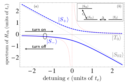
Figure 8: (color online). (a) Spectrum of the DQD Hamiltonian in the two-electron regime, as given in Eq.(28), as a function of the interdot detuning parameter $\epsilon$ for $\Delta=0$. Tunnel coupling between the singlet states $\left|S_{11}\right\rangle$ with (1,1) charge occupation and $\left|S_{02}\right\rangle$ with (0,2) charge occupation yields the hybridized singlet states $\left|S_{\pm}\right\rangle$. The ellipse refers to the qubit subspace, spanned by $\left|T_{0}\right\rangle$ and $\left|S_{-}\right\rangle$, while the dotted line (red) refers to the effective exchange coupling $J\left(\epsilon\right)=t_{c}^{2}/4\epsilon$. The arrows indicate schematically how to turn on and off the effective spin resonator coupling, by changing the effective dipole moment associated with the qubit. Inset (b): Relevant level diagram in the subspace $\left\{\left|T_{0}\right\rangle,\left|S_{11}\right\rangle,\left|S_{02}\right\rangle\right\}$.

We focus on the typical regime of interest, where (following the standard notation) the relevant electronic levels are given by the triplet states $\left|T_{+}\right\rangle=\left|\Uparrow\Uparrow\right\rangle$, $\left|T_{-}\right\rangle=\left|\Downarrow\Downarrow\right\rangle$, and $\left|T_{0}\right\rangle=\left(\left|\Uparrow\Downarrow\right\rangle+\left|\Downarrow\Uparrow\right\rangle\right)/\sqrt{2}$, as well as the singlet states $\left|S_{11}\right\rangle=\left(\left|\Uparrow\Downarrow\right\rangle-\left|\Downarrow\Uparrow\right\rangle\right)/\sqrt{2}$ and $\left|S_{02}\right\rangle=d_{R\uparrow}^{\dagger}d_{R\downarrow}^{\dagger}\left|0\right\rangle$ with $\left|\sigma\sigma^{\prime}\right\rangle=d_{L\sigma}^{\dagger}d_{R\sigma^{\prime}}^{\dagger}\left|0\right\rangle$; the fermionic creation (annihilation) operators $d_{i\sigma}^{\dagger}\left(d_{i\sigma}\right)$ create (annihilate) an electron with spin $\sigma=\uparrow,\downarrow$ in the orbital $i=L,R$. For sufficiently large magnetic field $B$, the levels $\left|T_{+}\right\rangle$ and $\left|T_{-}\right\rangle$ are far detuned and can be neglected for the remainder of the discussion. Therefore, in the following, we restrict ourselves to the subspace $\left\{\left|T_{0}\right\rangle,\left|S_{11}\right\rangle,\left|S_{02}\right\rangle\right\}$, as schematically depicted in the inset of Fig.8. In the relevant regime of interest, the electronic DQD system is described by the Hamiltonian taylor06

$$H_{\mathrm{DQD}} = \frac{t_{c}}{2}\left(\left|S_{02}\right\rangle\left\langle S_{11}\right|+\mathrm{h.c.}\right)+\Delta\left(\left|T_{0}\right\rangle\left\langle S_{11}\right|+\mathrm{h.c.}\right)$$ (28)

$$-\epsilon\left|S_{02}\right\rangle\left\langle S_{02}\right|,$$

where (as before) $t_{c}$ refers to the interdot tunneling amplitude, $\epsilon$ is the interdot detuning parameter, and $\Delta$ is a static magnetic field gradient between the two dots which couples singlet and triplet states. State preparation, measurement, single-qubit gates and local two-qubit gates can be achieved by tuning the bias $\epsilon$ hanson07-sm . Tunnel coupling between the singlet states $\left|S_{11}\right\rangle$ with (1,1) charge occupation and $\left|S_{02}\right\rangle$ with (0,2) charge occupation (here, $\left(m,n\right)$ refers to a configuration with $m(n)$ electrons in the left (right) dot, respectively) yields the hybridized singlet states $\left|S_{\pm}\right\rangle$, given by

$$\left|S_{+}\right\rangle = \cos\theta\left|S_{11}\right\rangle+\sin\theta\left|S_{02}\right\rangle,$$ (29)

$$\left|S_{-}\right\rangle = -\sin\theta\left|S_{11}\right\rangle+\cos\theta\left|S_{02}\right\rangle,$$ (30)

with $\tan\theta=t_{c}/\left(\epsilon+\Omega\right)$, $\Omega=\sqrt{\epsilon^{2}+t_{c}^{2}}$ and the associated eigenenergies $\epsilon_{\pm}=1/2\left(-\epsilon\pm\sqrt{\epsilon^{2}+t_{c}^{2}}\right)$. For large, negative detuning values ($\left|\epsilon\right|\gg t_{c}$), the splitting between the triplet $\left|T_{0}\right>$ and the hybridized singlet $\left|S_{-}\right\rangle$ can be approximated very well by the effective (tunable) exchange splitting $J\left(t_{c},\epsilon\right)=t_{c}^{2}/4\epsilon$; compare Fig.8. As schematically denoted by the ellipse in Fig.8, we focus on the regime where the singlet $\left|S_{+}\right\rangle$ is far off-resonance, yielding the effective qubit subspace $\left\{\left|T_{0}\right\rangle,\left|S_{-}\right\rangle\right\}$ with a qubit level splitting $\omega_{q}\approx J\left(t_{c},\epsilon\right)$.

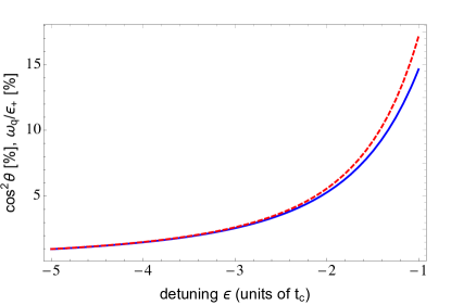
Figure 9: (color online). Effective spin resonator coupling $g_{\mathrm{sp}}/g_{0}=\cos^{2}\theta$ (solid blue line) and qubit level splitting $\omega_{q}\approx\left|J\right|$ relative to $\epsilon_{+}$ (dashed red line) as a function of the interdot detuning parameter $\epsilon$. The spin resonator coupling may reach a few percent of the bare charge resonator coupling $g_{0}$, with a qubit frequency $\omega_{q}$ that is much smaller than the energy of the level $\left|S_{+}\right\rangle$.

Again we consider a resonator with a single relevant mode of frequency $\omega_{c}$, as modeled by the Hamiltonian

$$H_{\mathrm{cav}}=\omega_{c}a^{\dagger}a.$$ (31)

In order to couple the electric field associated with the resonator mode to the electron spin states, the essential idea is to make use of an effective electric dipole moment associated with the exchange-coupled spin states of the DQD taylor06 . The resonator mode interacts capacitively with the double quantum dot taylor06 , as described by the interaction Hamiltonian $H_{I}=g_{0}\left|S_{02}\right\rangle\left\langle S_{02}\right|\otimes\left(a+a^{\dagger}\right)$. Projection onto the electronic low-energy subspace $\left\{\left|T_{0}\right\rangle,\left|S_{-}\right\rangle\right\}$ (i.e., projecting out the high-energy level $\left|S_{+}\right\rangle$) then leads (to lowest order in $\sim g_{0}/\epsilon_{+}$) to the effective spin resonator system

$$H = J\left|S_{-}\right\rangle\left\langle S_{-}\right|-\Delta\sin\theta\left(\left|T_{0}\right\rangle\left\langle S_{-}\right|+\mathrm{h.c.}\right)+\omega_{c}a^{\dagger}a$$ (32)

$$+g_{0}\cos^{2}\theta\left|S_{-}\right\rangle\left\langle S_{-}\right|\otimes\left(a+a^{\dagger}\right),$$

which includes a tunable spin resonator coupling, explicitly given by

$$g_{\mathrm{sp}}/g_{0}=\cos^{2}\theta=\frac{1}{2}\left(1+\frac{\epsilon}{\sqrt{\epsilon^{2}+t_{c}^{2}}}\right).$$ (33)

As demonstrated in Fig.9, the effective coupling $g_{\mathrm{sp}}$ may be turned on and off by sweeping the detuning parameter $\epsilon$ (closely following the functional dependence of $\omega_{q}/\epsilon_{+}$), i.e. by controlling the admixture of $\left|S_{02}\right\rangle$ to the hybridized singlet level $\left|S_{-}\right\rangle$. For large, negative values of $\epsilon$ this admixture vanishes $\left(\cos^{2}\theta\rightarrow 0\right)$, such that the effective dipole moment associated with the qubit vanishes and therefore the spin-resonator coupling is switched off. The type of spin-resonator coupling (transversal versus longitudinal) may be controlled by the magnetic gradient $\Delta$, as can be done using e.g. a nanomagnet or nuclear Overhauser fields hanson07-sm ; beaudoin16 . While for longitudinal spin-resonator coupling the resonator frequency $\omega_{c}$ may be comparable or even smaller than the effective qubit level splitting $J$ (see Sec.H for details), in the case of transversal coupling the effective qubit level splitting needs to be much smaller than the cavity frequency, that is $|J\left(t_{c},\epsilon\right)|\approx|t_{c}^{2}/4\epsilon|\ll\omega_{c}$, but, at the same time, $\epsilon_{+}\approx\left|\epsilon\right|+t_{c}^{2}/4\left|\epsilon\right|\gg\omega_{c}$ should be fulfilled in order to neglect the high-energy level $\left|S_{+}\right\rangle$. Still, both requirements can be satisfied by choosing the parameters as $t_{c},\omega_{c}\ll\left|\epsilon\right|$.

Appendix E Spin-Spin Coupling in Dispersive Regime

We consider two identical spins homogeneously coupled to a common resonator mode. The dynamics are assumed to be governed by the Jaynes-Cummings Hamiltonian

$$H=\Delta\left(S_{1}^{z}+S_{2}^{z}\right)+g\left[a\left(S_{1}^{+}+S_{2}^{+}\right)+a^{\dagger}\left(S_{1}^{-}+S_{2}^{-}\right)\right],$$ (34)

which is valid within the rotating-wave approximation for $\sqrt{\bar{n}_{\mathrm{th}}}g,\Delta\ll\omega_{c}$, with the detuning $\Delta=\omega_{q}-\omega_{c}$. In the following we consider the dispersive regime, where the spin-resonator coupling is strongly detuned $\left(\sqrt{\bar{n}_{\mathrm{th}}}g\ll\Delta\right)$. In this regime, the spin-resonator coupling can be treated perturbatively. To stress the perturbative treatment we write

$$H = H_{0}+H_{1},$$ (35)

$$H_{0} = \Delta S^{z},$$ (36)

$$H_{1} = g\left(aS^{+}+a^{\dagger}S^{-}\right),$$ (37)

where $S^{\alpha}=S_{1}^{\alpha}+S_{2}^{\alpha}$ (for $\alpha=\pm,z$) are collective spin operators. We perform a standard Schrieffer-Wolff transformation

$$\tilde{H} = e^{A}He^{-A}$$ (38)

$$\approx H_{0}+H_{1}+\left[A,H_{0}+H_{1}\right]+\frac{1}{2}\left[A,\left[A,H_{0}\right]\right],$$ (39)

where the operator $A$ (with $A^{\dagger}=-A$) is assumed to have a perturbative expansion in $g$, i.e., $A=0+\mathcal{O}\left(g\right)+\dots$ By choosing

$$\left[A,H_{0}\right]=-H_{1},$$ (40)

one obtains a Hamiltonian $\tilde{H}$ without linear coupling in $g$,

$$\tilde{H}\approx H_{0}+\frac{1}{2}\left[A,H_{1}\right].$$ (41)

For the Hamiltonian given in Eq.(35), the condition in Eq.(40) is fulfilled by the choice

$$A=\frac{g}{\Delta}\left(aS^{+}-a^{\dagger}S^{-}\right),$$ (42)

which yields the Hamiltonian

$$\tilde{H}\approx\left(\Delta+\frac{g^{2}}{\Delta}+2\frac{g^{2}}{\Delta}a^{\dagger}a\right)S^{z}+\frac{g^{2}}{\Delta}\left(S_{1}^{+}S_{2}^{-}+S_{1}^{-}S_{2}^{+}\right).$$ (43)

Here, the last two terms describe a cavity-state dependent dispersive shift of the qubit transition frequencies and spin-spin coupling via virtual occupation of the cavity mode, respectively. The strength of the effective spin-spin coupling is given by

$$g_{\mathrm{eff}}=\frac{g^{2}}{\Delta}=\frac{\epsilon}{\sqrt{\bar{n}_{\mathrm{th}}}}g,$$ (44)

where we have set $\sqrt{\bar{n}_{\mathrm{th}}}g/\Delta=\epsilon\ll 1$ in order to reach the regime of validity for Eq.(43), given by

$$\sqrt{\bar{n}_{\mathrm{th}}}g\ll\Delta\ll\omega_{c}.$$ (45)

By transforming the Hamiltonian given in Eq.(43) back into the lab-frame, we recover the result presented in Ref.blais04 , namely

$$H \approx \left[\omega_{c}+2\frac{g^{2}}{\Delta}\left(S_{1}^{z}+S_{2}^{z}\right)\right]a^{\dagger}a+\left(\omega_{q}+\frac{g^{2}}{\Delta}\right)\left(S_{1}^{z}+S_{2}^{z}\right)$$ (46)

$$+\frac{g^{2}}{\Delta}\left(S_{1}^{+}S_{2}^{-}+S_{1}^{-}S_{2}^{+}\right).$$

Here, spins and cavity mode are still coupled by the ac Stark shift term $\sim a^{\dagger}a$. Accordingly, one obtains an effective pure spin Hamiltonian with flip-flop interactions provided that one can neglect any fluctuations of the photon number $a^{\dagger}a\rightarrow\bar{n}=\left\langle a^{\dagger}a\right\rangle$, where $\bar{n}$ is the average number of photons in the cavity mode trif08 .

Since the operator $S^{z}a^{\dagger}a$ in Eq.(43) has an integer spectrum, one may wonder whether for stroboscopic times the spins disentangle from the resonator mode here as well. Thus, let us consider the full time evolution generated by Eq.(34)

$$e^{-iHt} = e^{-iU^{\dagger}\tilde{H}Ut}=U^{\dagger}e^{-i\tilde{H}t}U$$ (47)

$$\approx U^{\dagger}\left[\exp\left[-it\left(\delta+\tilde{\delta}a^{\dagger}a\right)S^{z}\right.\right.$$

$$\left.\left.-i\tilde{g}t\left(S_{1}^{+}S_{2}^{-}+S_{1}^{-}S_{2}^{+}\right)\right]\right]U,$$

with $U=\exp\left(A\right)$, $\delta=\Delta+g^{2}/\Delta$, $\tilde{\delta}=2g^{2}/\Delta$ and $\tilde{g}=g^{2}/\Delta$. Note that Eq.(E) is an approximate statement, relying on a perturbative expansion in the coupling $g$. Since the flip-flop interaction conserves $S^{z}$, we find

$$e^{-iHt}\approx U^{\dagger}e^{-i\delta tS^{z}}e^{-i\tilde{\delta}tS^{z}a^{\dagger}a}e^{-i\tilde{g}t\left(S_{1}^{+}S_{2}^{-}+S_{1}^{-}S_{2}^{+}\right)}U.$$ (49)

For stroboscopic times $\tilde{\delta}t=2\pi m$, $e^{-i\tilde{\delta}tS^{z}a^{\dagger}a}=\mathds{1}$, yielding

$$e^{-iHt}\approx U^{\dagger}e^{-iH_{\mathrm{spin}}t}U,$$ (50)

where $H_{\mathrm{spin}}=\delta S^{z}+\tilde{g}\left(S_{1}^{+}S_{2}^{-}+S_{1}^{-}S_{2}^{+}\right)$ is a pure spin Hamiltonian, without any coupling to the resonator mode. However, in contrast to our scheme presented in the main text, the full time evolution does not reduce to a pure spin problem, since the Schrieffer-Wolff transformation $U=\exp\left[\frac{g}{\Delta}\left(aS^{-}-a^{\dagger}S^{+}\right)\right]$ does not commute with $e^{-iH_{\mathrm{spin}}t}$, but rather entangles the qubits with the resonator mode.

Appendix F Schrieffer-Wolff Transformation

If one restricts oneself to the regime $g\ll\omega_{c}$, the result stated in Eqn.(6) may also be derived in the perturbative framework of a Schrieffer-Wolff transformation. For concreteness, assuming $\omega_{q}=0$, we consider the Hamiltonian

$$H=\underset{H_{0}}{\underbrace{\omega_{c}a^{\dagger}a}}+\underset{V}{\underbrace{gS^{x}\otimes\left(a+a^{\dagger}\right)}},$$ (51)

where $S^{x}=\sum_{i}\eta_{i}^{x}\sigma_{i}^{x}$ is a collective operator. In the following, and contrary to our general analysis in the main text, we restrict ourselves to the regime where the spin-resonator coupling $V$ can be treated perturbatively with respect to $H_{0}$, that is $g\ll\omega_{c}$. Performing a Schrieffer-Wolff transformation $\tilde{H}=e^{A}He^{-A}$ as presented in Sec. E, with $A=-\frac{g}{\omega_{c}}S^{x}\left(a-a^{\dagger}\right)$, we obtain an effective Hamiltonian $\tilde{H}$ where the slow subspace is decoupled from the fast subspace up to second order in $g$. Explicitly it reads [compare Eq.(5)]

$$\tilde{H}\approx\omega_{c}a^{\dagger}a-\frac{g^{2}}{\omega_{c}}S_{x}^{2}.$$ (52)

Appendix G Non-Zero Qubit Level Splitting

In our derivation of Eq.(5), starting from the generic spin-resonator Hamiltonian given in Eq.(1), we have assumed $\omega_{q}=0$. As demonstrated also numerically in Section K below, small level splittings with $\omega_{q}\approx 0.1\omega_{c}$ may still be tolerated without a significant loss in the amount of generated entanglement and the fidelity with the maximally entangled target state.

In this Appendix we investigate analytically the effects associated with a finite splitting $\omega_{q}>0$. In this case, Eq.(3) can be generalized straightforwardly to

$$H=U[\underset{H_{0}}{\underbrace{\omega_{c}a^{\dagger}a-\frac{g^{2}}{\omega_{c}}\mathcal{S}^{2}}}+\frac{\omega_{q}}{2}\tilde{S}^{z}]U^{\dagger},$$ (53)

where $\tilde{S}^{z}=U^{\dagger}S^{z}U$, with $U=\exp\left[\frac{g}{\omega_{c}}\mathcal{S}\left(a-a^{\dagger}\right)\right]$. In what follows, we restrict ourselves to the (experimentally) most relevant regime where $\mu=g/\omega_{c}\ll 1$, which allows for a simple perturbative treatment. Expansion in the small parameter $\mu$ yields

$$\tilde{S}^{z}\approx S^{z}-\mu\left(a-a^{\dagger}\right)\left[\mathcal{S},S^{z}\right]+\frac{\mu^{2}}{2}\left(a-a^{\dagger}\right)^{2}\left[\mathcal{S},\left[\mathcal{S},S^{z}\right]\right].$$ (54)

Specifically, for $\mathcal{S}=\sum_{i}\sigma_{i}^{x}$ (as considered in the main text) we then obtain

$$\tilde{S}^{z}\approx S^{z}+2i\frac{g}{\omega_{c}}S^{y}\left(a-a^{\dagger}\right)+2\left(\frac{g}{\omega_{c}}\right)^{2}S^{z}\left(a-a^{\dagger}\right)^{2},$$ (55)

which leads to an additional (undesired) contribution in Eq.(53) of the form

$$\frac{\omega_{q}}{2}\tilde{S}^{z}\approx\frac{\omega_{q}}{2}S^{z}+\epsilon\left[igS^{y}\left(a-a^{\dagger}\right)+\frac{g^{2}}{\omega_{c}}S^{z}\left(a-a^{\dagger}\right)^{2}\right].$$ (56)

Here, in contrast to the ideal Hamiltonian $H_{0}$ in Eq.(53) the spins are not decoupled from the (hot) resonator mode. However, apart from being detuned by at least $\omega_{c}-\omega_{q}$, the undesired terms—that lead to entanglement of the spins with the (hot) resonator mode—are suppressed by the small parameter $\epsilon=\omega_{q}/\omega_{c}\ll 1$. In the limit $\omega_{q}\rightarrow 0$ $\left(\epsilon\rightarrow 0\right)$ we recover the ideal dynamics.

Appendix H Errors due to Non-Zero Qubit-Level Splitting

In this Appendix we analyze errors induced by a non-zero qubit level splitting $\left(\omega_{q}/\omega_{c}>0\right)$. In the case of longitudinal spin-resonator coupling, we show that controlled phase gates can be implemented (as described in the main text for $\omega_{q}=0$), even in the presence of non-zero and inhomogeneous qubit level splittings $\left(\omega_{q}>0\right)$, when applying either fast local single qubit gates (to correct the effect of known $\omega_{q}\neq 0$) or standard spin-echo techniques (to compensate unknown detunings); see section H.1. Therefore, for longitudinal spin-resonator coupling, our approach yields a high-fidelity hot gate, that is independent of the qubit level splitting $\omega_{q}/\omega_{c}\geq 0$. As detailed in section H.2, this is not the case for transversal coupling, where $\omega_{q}\neq 0$ causes second order errors, which, however, are suppressed in certain decoherence-free subspaces. Thus, as opposed to the limiting regime where $\omega_{q}=0$, the distinction between longitudinal and transversal spin-resonator coupling indeed becomes meaningful.

The model.—In the absence of other error sources $\left(\kappa=\Gamma=0\right)$, the system’s dynamics are governed by the Hamiltonian

$$H = H_{0}+V,$$ (57)

$$H_{0} = \omega_{c}a^{\dagger}a+g\mathcal{S}\otimes\left(a+a^{\dagger}\right),$$ (58)

$$V = \frac{\omega_{q}}{2}S^{z},$$ (59)

with $S^{z}=\sum_{i}\sigma_{i}^{z}$ and $\mathcal{S}=\sum_{i,\alpha}\eta_{i}^{\alpha}\sigma_{i}^{\alpha}$. Below, we will set $S^{\alpha}=S_{\alpha}$ $\left(\alpha=x,z\right)$ interchangeably. Also, note that $S^{x},S^{z}$ as defined here refer to the usual spin operators muliplied by 2.

H.1 Longitudinal Spin-Resonator Coupling

Controlled phase gate.—Let us first focus on the case of longitudinal spin-resonator coupling, where $\mathcal{S}=\sum_{i}\sigma_{i}^{z}=S^{z}$ and accordingly $\left[H_{0},V\right]=0$. In this scenario, controlled phase gates can be implemented (as described in the main text for $\omega_{q}=0$), even in the presence of non-zero qubit level splittings $\left(\omega_{q}>0\right)$, when applying either fast local single qubit phase-gates (to correct the effect of known $\omega_{q}\neq 0$) or standard spin-echo techniques (to compensate unknown detunings). By flipping the qubits (for example) halfway the evolution and at the end of the gate, the effect of $V$ is canceled exactly. Denoting such a global flip of all qubits around the axis $\alpha=x,y,z$ as $U_{\alpha}\left(\varphi\right)=\exp\left[-i\varphi/2\sigma_{1}^{\alpha}\right]\dots\exp\left[-i\varphi/2\sigma_{N}^{\alpha}\right]=\exp\left[-i\varphi/2\sum\sigma_{i}^{\alpha}\right]$, for two qubits the full evolution (in the computational basis {$\left|00\right\rangle,\left|10\right\rangle,\left|01\right\rangle,\left|11\right\rangle$}), intertwined by spin echo pulses, reads

$$U\left(2t_{m}\right) = U_{x}\left(\pi\right)e^{-iHt_{m}}U_{x}\left(\pi\right)e^{-iHt_{m}},$$ (60)

$$= \mathrm{diag}\left(e^{i\phi},1,1,e^{i\phi}\right),$$ (61)

with $\phi=16m\pi\mu^{2}$. The gate $U\left(2t_{m}\right)$ is independent of the resonator mode and, as a consequence of the spin-echo $\pi$-pulses $U_{x}\left(\pi\right)$, independent of $\omega_{q}$; accordingly, the qubit level splittings do not have to be necessarily small. When complementing the propagator $U\left(2t_{m}\right)$ with local unitaries, such that $\left|0\right\rangle_{i}\rightarrow e^{-i\phi/2}\left|0\right\rangle_{i}$ and $\left|1\right\rangle_{i}\rightarrow e^{i\phi/2}\left|1\right\rangle_{i}$, we obtain

$$U_{\mathrm{Cphase}} = U_{z}\left(-\phi\right)U_{x}\left(\pi\right)e^{-iHt_{m}}U_{x}\left(\pi\right)e^{-iHt_{m}}$$ (62)

$$= \mathrm{diag}\left(1,1,1,e^{2i\phi}\right),$$ (63)

which yields a controlled phase gate for $\phi=\pi/2$ (corresponding to a gate time $t_{\max}=\pi/16g_{\mathrm{eff}}$), that is insensitive to the qubit level splittings $\omega_{q}>0$.

For longitudinal spin-resonator coupling, Eq.(5) of the main text simply reads

$$e^{-iHt_{m}}=\exp\left[i2\pi m\mu^{2}\tilde{\mathcal{S}}^{2}\right],$$ (64)

with (the generalized expression) $\tilde{\mathcal{S}}^{2}=\mathcal{S}^{2}-\left(\omega_{q}/2g_{\mathrm{eff}}\right)S^{z}$, where $\mathcal{S}=\sum_{i}\eta_{i}\sigma_{i}^{z}$, while the operator $S^{z}$ can also be generalized to account for possible inhomogeneities in the qubit level splittings (with $\omega_{q,i}=\delta_{i}\omega_{q}$), i.e. $S^{z}\rightarrow\sum\delta_{i}\sigma_{i}^{z}$. This gate differs from the ideal one ($\exp\left[i2\pi m\mu^{2}\mathcal{S}^{2}\right]$) only by the local phases $\exp\left[-it_{m}(\omega_{q}/2)S^{z}\right]$ and thus has the same computational power.

H.2 Transversal Spin-Resonator Coupling

Transversal spin-resonator coupling.—In the following we turn to systems with transversal spin resonator coupling, where $\mathcal{S}=S^{x}=\sum_{i}\sigma_{i}^{x}$. In this case, the theoretical treatment is more involved as compared to our previous discussion on longitudinal spin resonator coupling, because the ideal free evolution does not commute with the perturbation ($\left[H_{0},V\right]\neq 0$). We use perturbative techniques to derive an analytic expression for the error $\xi_{q}$ induced by non-zero qubit splittings $\omega_{q}>0$. For the sake of readability, here we restrict ourselves to two qubits, while our analysis can be generalized readily to more than two qubits.

Perturbative series.—Up to second order in the perturbation $V$, the unitary evolution operator associated with $H$ is approximately given by

$$U\left(t\right) \approx e^{-iH_{0}t}\left[\mathbb{1}-i\int_{0}^{t}d\tau\tilde{V}\left(\tau\right)\right.$$ (65)

$$\left.-\int_{0}^{t}d\tau_{2}\int_{0}^{\tau_{2}}d\tau_{1}\tilde{V}\left(\tau_{2}\right)\tilde{V}\left(\tau_{1}\right)\right],$$

with

$$\tilde{V}\left(\tau\right)=e^{iH_{0}\tau}Ve^{-iH_{0}\tau}.$$ (66)

Initially, the resonator mode is assumed to be in a thermal state $\rho_{\mathrm{th}}=\rho_{\mathrm{th}}\left(T\right)=Z^{-1}\exp\left[-\beta\omega_{c}a^{\dagger}a\right]$. Then, starting from the initial state $\rho\left(0\right)=\varrho\left(0\right)\otimes\rho_{\mathrm{th}}$, the system (comprising both spin and resonator degrees of freedom) evolves as

$$\rho\left(t\right)=U\left(t\right)\varrho\left(0\right)\rho_{\mathrm{th}}U^{\dagger}\left(t\right).$$ (67)

Inserting the perturbative expansion given in Eq.(65), up to second order in $V$ we obtain

$$\rho\left(t\right) \approx e^{-iH_{0}t}\left\{\rho\left(0\right)-i\int_{0}^{t}d\tau\left[\tilde{V}\left(\tau\right),\rho\left(0\right)\right]\right.$$ (68)

$$+\int_{0}^{t}d\tau\int_{0}^{t}d\tau^{\prime}\tilde{V}\left(\tau\right)\rho\left(0\right)\tilde{V}\left(\tau^{\prime}\right)$$

$$-\int_{0}^{t}d\tau_{2}\int_{0}^{\tau_{2}}d\tau_{1}\tilde{V}\left(\tau_{2}\right)\tilde{V}\left(\tau_{1}\right)\rho\left(0\right)$$

$$\left.-\int_{0}^{t}d\tau_{2}\int_{0}^{\tau_{2}}d\tau_{1}\rho\left(0\right)\tilde{V}\left(\tau_{1}\right)\tilde{V}\left(\tau_{2}\right)\right\}e^{iH_{0}t}.$$

Eigensystem of unperturbed Hamiltonian.—In the first step, it it instructive to find the eigensystem of $H_{0}$. Following the same strategy as outlined in the main text, $H_{0}$ can be written as

$$H_{0}=D^{\dagger}(\mu S^{x})\left[\omega_{c}a^{\dagger}a-g_{\mathrm{eff}}S_{x}^{2}\right]D(\mu S^{x}),$$ (69)

where $\mu=g/\omega_{c}$, $g_{\mathrm{eff}}=g^{2}/\omega_{c}=\mu^{2}\omega_{c}$ and $D\left(\alpha\right)=\exp\left[\alpha a^{\dagger}-\alpha^{*}a\right]$ is a displacement operator. Accordingly, the eigensystem of $H_{0}$ is found to be

$$H_{0}\widetilde{\left|n,\vec{\sigma}_{x}\right\rangle}=E_{n,s}\widetilde{\left|n,\vec{\sigma}_{x}\right\rangle},$$ (70)

where the eigenvectors are given by product states of spins aligned along the transversal direction $x$ and displaced resonator states with a displacement proportional to the total spin projection $s$ along $x$,

$$\widetilde{\left|n,\vec{\sigma}_{x}\right\rangle}=D^{\dagger}\left(\mu s\right)\left|n\right\rangle\otimes\left|\vec{\sigma}_{x}\right\rangle,$$ (71)

with $s=s_{1}^{x}+s_{2}^{x}$, $S^{x}\left|\vec{\sigma}_{x}\right\rangle=\left(s_{1}^{x}+s_{2}^{x}\right)\left|\vec{\sigma}_{x}\right\rangle$ and $\left|n\right\rangle$ denoting the usual Fock states. The corresponding eigenenergies

$$E_{n,s}=n\omega_{c}-s^{2}g_{\mathrm{eff}},$$ (72)

refer to manifolds with fixed resonator excitation number $n=0,1,2,\dots$ and two-qubit spin states with a resonator-induced splitting of $4g_{\mathrm{eff}}$ between the states $\left\{\left|\uparrow_{x},\downarrow_{x}\right\rangle,\left|\downarrow_{x},\uparrow_{x}\right\rangle\right\}$ with $s^{2}=0$ and $\left\{\left|\uparrow_{x},\uparrow_{x}\right\rangle,\left|\downarrow_{x},\downarrow_{x}\right\rangle\right\}$ with $s^{2}=4$, respectively.

Perturbation in the interaction picture.—In the following we focus on the perturbative regime where the perturbation $\sim\omega_{q}$ is small compared to the resonator-induced splitting of $S_{x}^{2}$-eigenstates, that is $\omega_{q}\ll 8g_{\mathrm{eff}}=8\mu^{2}\omega_{c}$. Rewriting the perturbation in the unperturbed eigenbasis yields

$$V=\sum_{n,n^{\prime}}\sum_{\vec{\sigma},\vec{\sigma}^{\prime}}\left<n^{\prime}|D\left[\mu\left(s^{\prime}-s\right)\right]|n\right>\left<\vec{\sigma}_{x}^{\prime}|V|\vec{\sigma}_{x}\right>\widetilde{\left|n^{\prime},\vec{\sigma}^{\prime}_{x}\right\rangle}\widetilde{\left\langle n,\vec{\text{$\sigma$}}_{x}\right|}.$$ (73)

Using the relation cahill69

$$\left<m|D\left[\alpha\right]|n\right>=\sqrt{\frac{n!}{m!}}\alpha^{m-n}e^{-\left|\alpha\right|^{2}/2}L_{n}^{(m-n)}\left(\left|\alpha\right|^{2}\right),$$ (74)

with $L_{n}^{(m-n)}$ denoting the associated Laguerre polynominals, in the experimentally most relevant regime of weak spin-resonator coupling (that is, $\mu\ll 1$) we can neglect the off-diagonal contributions where $n\neq m$, since eigenstates with different boson number are very weakly coupled $\left(\sim\omega_{q}\mu^{|n-m|}\right)$ and far off-resonance $\left(\omega_{q}\ll 8g_{\mathrm{eff}}\ll\omega_{c}\right)$, with rapidly decaying contributions as the number difference increases. In this limit, the perturbation in the interaction picture [compare Eq.(66)] reads

$$\tilde{V}\left(\tau\right) \approx \tilde{V}_{q}\left(\tau\right)\otimes\sum_{n}\chi_{n}\left(\mu\right)\left|n\right\rangle\left\langle n\right|,$$ (75)

$$\tilde{V}_{q}\left(\tau\right) = \frac{\omega_{q}}{2}\left[e^{i4g_{\mathrm{eff}}\tau}Q+e^{-i4g_{\mathrm{eff}}\tau}Q^{\dagger}\right],$$ (76)

where

$$\chi_{n}\left(\mu\right)=\left<n|D\left[\pm 2\mu\right]|n\right>=e^{-2\mu^{2}}L_{n}^{(0)}\left(4\mu^{2}\right),$$ (77)

Since the perturbation $\sim S^{z}$ is purely off-diagonal in the $S^{x}$ eigenbasis, the operator

$$Q = \left|\uparrow_{x}\downarrow_{x}\right\rangle\left\langle\downarrow_{x}\downarrow_{x}\right|+\left|\downarrow_{x}\uparrow_{x}\right\rangle\left\langle\downarrow_{x}\downarrow_{x}\right|$$ (78)

$$+\left|\uparrow_{x}\downarrow_{x}\right\rangle\left\langle\uparrow_{x}\uparrow_{x}\right|+\left|\downarrow_{x}\uparrow_{x}\right\rangle\left\langle\uparrow_{x}\uparrow_{x}\right|,$$

describes only transitions from the $s=\pm 2$ subspace to the $s=0$ subspace (and vice versa for the Hermitian conjugate operator $Q^{\dagger}$), which in the interaction picture underlying Eq.(76) rotate with the corresponding transition frequency $\pm 4g_{\mathrm{eff}}$. While Eq.(75) is purely off-diagonal in spin-space, in the limit $\mu\ll 1$ it is (approximately) diagonal in the excitation number $\left|n\right\rangle$, as the coupling $V$ between different $n$-subspaces is strongly detuned by the corresponding large energy splitting $\sim\omega_{c}$.

Quasi-decoherence-free subspace.—In our numerical simulations, the initial qubit states have been chosen to be aligned along the $z$-direction, defining the computational basis states and corresponding to eigenstates of the perturbation $V\sim S^{z}$. Therefore, it is didactic to rewrite $\tilde{V}\left(\tau\right)$ in the eigenbasis of $S^{z}$. With $\left|\uparrow_{x}\right\rangle=\left(\left|\uparrow_{z}\right\rangle+\left|\downarrow_{z}\right\rangle\right)/\sqrt{2}$, and $\left|\downarrow_{x}\right\rangle=\left(\left|\uparrow_{z}\right\rangle-\left|\downarrow_{z}\right\rangle\right)/\sqrt{2}$, we obtain

$$Q = \left|\uparrow_{z}\uparrow_{z}\right\rangle\left\langle\uparrow_{z}\uparrow_{z}\right|-\left|\downarrow_{z}\downarrow_{z}\right\rangle\left\langle\downarrow_{z}\downarrow_{z}\right|$$ (79)

$$+\left|\uparrow_{z}\uparrow_{z}\right\rangle\left\langle\downarrow_{z}\downarrow_{z}\right|-\left|\downarrow_{z}\downarrow_{z}\right\rangle\left\langle\uparrow_{z}\uparrow_{z}\right|.$$

As can be seen readily from this expression, the subspace $\left\{\left|\uparrow_{z}\downarrow_{z}\right\rangle,\left|\downarrow_{z}\uparrow_{z}\right\rangle\right\}$ with $S^{z}=0$ defines a decoherence-free subspace, since $Q$ and $Q^{\dagger}$ [and therefore $\tilde{V}\left(\tau\right)$] vanish on this subspace, with $Q\left|\uparrow_{z}\downarrow_{z}\right\rangle=Q\left|\downarrow_{z}\uparrow_{z}\right\rangle=0$. In the following this finding is elaborated in more detail: To do so, we first rewrite $\tilde{V}\left(\tau\right)$ as

$$\tilde{V}\left(\tau\right) = \frac{\omega_{q}}{2}D^{\dagger}(\mu S^{x})e^{i\omega_{c}a^{\dagger}a\tau}e^{-ig_{\mathrm{eff}}\tau S_{x}^{2}}D(\mu S^{x})S^{z}$$ (80)

$$\times D^{\dagger}(\mu S^{x})e^{-i\omega_{c}a^{\dagger}a\tau}e^{ig_{\mathrm{eff}}\tau S_{x}^{2}}D(\mu S^{x}).$$

This expression is exact. Defining triplet and singlet states in the spin-eigenbasis of $H_{0}$ as

$$\left|T_{+}^{x}\right\rangle = \left|\uparrow_{x}\uparrow_{x}\right\rangle,$$ (81)

$$\left|T_{0}^{x}\right\rangle = \left(\left|\uparrow_{x}\downarrow_{x}\right\rangle+\left|\downarrow_{x}\uparrow_{x}\right\rangle\right)/\sqrt{2},$$ (82)

$$\left|T_{-}^{x}\right\rangle = \left|\downarrow_{x}\downarrow_{x}\right\rangle,$$ (83)

$$\left|S^{x}\right\rangle = \left(\left|\uparrow_{x}\downarrow_{x}\right\rangle-\left|\downarrow_{x}\uparrow_{x}\right\rangle\right)/\sqrt{2},$$ (84)

the (by definition) computational basis states (taken as initial states in our numerical simulations) are given by

$$\left|\uparrow_{z}\uparrow_{z}\right\rangle = \frac{1}{2}\left[\left|T_{+}^{x}\right\rangle+\sqrt{2}\left|T_{0}^{x}\right\rangle+\left|T_{-}^{x}\right\rangle\right],$$ (85)

$$\left|\uparrow_{z}\downarrow_{z}\right\rangle = \frac{1}{2}\left[\left|T_{+}^{x}\right\rangle-\sqrt{2}\left|S^{x}\right\rangle-\left|T_{-}^{x}\right\rangle\right],$$ (86)

$$\left|\downarrow_{z}\uparrow_{z}\right\rangle = \frac{1}{2}\left[\left|T_{+}^{x}\right\rangle+\sqrt{2}\left|S^{x}\right\rangle-\left|T_{-}^{x}\right\rangle\right],$$ (87)

$$\left|\downarrow_{z}\downarrow_{z}\right\rangle = \frac{1}{2}\left[\left|T_{+}^{x}\right\rangle-\sqrt{2}\left|T_{0}^{x}\right\rangle+\left|T_{-}^{x}\right\rangle\right].$$ (88)

For a general resonator state $\left|\mathrm{cav}\right\rangle$, the first-order error term will be proportional to

$$\tilde{V}\left(\tau\right)\left|T_{+}^{x}\right\rangle\left|\mathrm{cav}\right\rangle = \frac{\omega_{q}}{\sqrt{2}}e^{4ig_{\mathrm{eff}}\tau}\left|T_{0}^{x}\right\rangle\otimes e^{i\omega_{c}a^{\dagger}a\tau}D^{\dagger}(2\mu)e^{-i\omega_{c}a^{\dagger}a\tau}D(2\mu)\left|\mathrm{cav}\right\rangle,$$ (89)

$$\tilde{V}\left(\tau\right)\left|T_{0}^{x}\right\rangle\left|\mathrm{cav}\right\rangle = \frac{\omega_{q}}{\sqrt{2}}e^{-4ig_{\mathrm{eff}}\tau}\left[\left|T_{+}^{x}\right\rangle\otimes D^{\dagger}(2\mu)e^{i\omega_{c}a^{\dagger}a\tau}D(2\mu)e^{-i\omega_{c}a^{\dagger}a\tau}\left|\mathrm{cav}\right\rangle\right.$$ (90)

$$\left.+\left|T_{-}^{x}\right\rangle\otimes D^{\dagger}(-2\mu)e^{i\omega_{c}a^{\dagger}a\tau}D(-2\mu)e^{-i\omega_{c}a^{\dagger}a\tau}\left|\mathrm{cav}\right\rangle\right],$$

$$\tilde{V}\left(\tau\right)\left|T_{-}^{x}\right\rangle\left|\mathrm{cav}\right\rangle = \frac{\omega_{q}}{\sqrt{2}}e^{4ig_{\mathrm{eff}}\tau}\left|T_{0}^{x}\right\rangle\otimes e^{i\omega_{c}a^{\dagger}a\tau}D^{\dagger}(-2\mu)e^{-i\omega_{c}a^{\dagger}a\tau}D(-2\mu)\left|\mathrm{cav}\right\rangle$$ (91)

$$\tilde{V}\left(\tau\right)\left|S^{x}\right\rangle\left|\mathrm{cav}\right\rangle = 0.$$ (92)

In the spirit of our previous discussion [recall Eq.(74) with $D^{\dagger}\left(\alpha\right)=D\left(-\alpha\right)$], these exact statements can be simplified in the limit $\mu\ll 1$ as

$$e^{i\omega_{c}a^{\dagger}a\tau}D^{\dagger}(\pm 2\mu)e^{-i\omega_{c}a^{\dagger}a\tau} = \sum_{n,n^{\prime}}e^{i\omega_{c}\tau\left(n^{\prime}-n\right)}\left<n^{\prime}|D^{\dagger}\left(\pm 2\mu\right)|n\right>\left|n^{\prime}\right\rangle\left\langle n\right|,$$ (93)

$$\approx \sum_{n}\chi_{n}\left(\mu\right)\left|n\right\rangle\left\langle n\right|,$$ (94)

yielding the approximate results [for a Fock state $\left|\mathrm{cav}\right\rangle=\left|n\right\rangle$]

$$\tilde{V}\left(\tau\right)\left|T_{+}^{x}\right\rangle\left|n\right\rangle \approx \frac{\omega_{q}}{\sqrt{2}}e^{4ig_{\mathrm{eff}}\tau}\chi_{n}^{2}\left(\mu\right)\left|T_{0}^{x}\right\rangle\left|n\right\rangle,$$ (95)

$$\tilde{V}\left(\tau\right)\left|T_{0}^{x}\right\rangle\left|n\right\rangle \approx \frac{\omega_{q}}{\sqrt{2}}e^{-4ig_{\mathrm{eff}}\tau}\chi_{n}^{2}\left(\mu\right)\left[\left|T_{+}^{x}\right\rangle+\left|T_{-}^{x}\right\rangle\right]\left|n\right\rangle,$$ (96)

$$\tilde{V}\left(\tau\right)\left|T_{-}^{x}\right\rangle\left|n\right\rangle \approx \frac{\omega_{q}}{\sqrt{2}}e^{4ig_{\mathrm{eff}}\tau}\chi_{n}^{2}\left(\mu\right)\left|T_{0}^{x}\right\rangle\left|n\right\rangle.$$ (97)

With these (approximate) relations, one can readily verify $\tilde{V}\left(\tau\right)\left|\uparrow_{z}\downarrow_{z}\right\rangle\left|n\right\rangle\approx 0$ and $\tilde{V}\left(\tau\right)\left|\downarrow_{z}\uparrow_{z}\right\rangle\left|n\right\rangle\approx 0$, in agreement with our result based on Eq.(79), while the subspace $\left\{\left|\uparrow_{z}\uparrow_{z}\right\rangle,\left|\downarrow_{z}\downarrow_{z}\right\rangle\right\}$ is directly affected by the perturbation $\tilde{V}\left(\tau\right)$. As long as transitions between different $n$-subspaces can be neglected, the bosonic part of the Hamiltonian can be ignored and the free part of the Hamiltonian reduces to $H_{0}\approx-g_{\mathrm{eff}}S_{x}^{2}$. Then, since the perturbation $V=(\omega_{q}/2)S^{z}$ leaves the subspace $\left\{\left|\uparrow_{z}\downarrow_{z}\right\rangle,\left|\downarrow_{z}\uparrow_{z}\right\rangle\right\}$ invariant, $V$ cannot induce errors, since it vanishes on this subspace. As a perspective, this finding opens up the possibility to define a logical qubit in the quasi-decoherence-free subspace $\left\{\left|\uparrow_{z}\downarrow_{z}\right\rangle,\left|\downarrow_{z}\uparrow_{z}\right\rangle\right\}$ as $\left|\mathrm{qubit}\right\rangle=\alpha\left|\uparrow_{z}\downarrow_{z}\right\rangle+\beta\left|\downarrow_{z}\uparrow_{z}\right\rangle$, which is largely protected from splitting-induced errors in the limit $\mu\ll 1$ (provided that the perturbative condition $\omega_{q}\ll 8g_{\mathrm{eff}}$ is still satisfied).

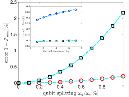
Figure 10: (color online). The error $\xi_{q}$ induced by a non-zero qubit splitting $\omega_{q}>0$, for $\mathcal{S}=S^{x}=\sum_{i}\sigma_{i}^{x}$ (transversal coupling), and for different initial qubit states $\left|\Psi(0)\right\rangle=\left|\uparrow_{z}\downarrow_{z}\right\rangle$ (red circles) and $\left|\Psi(0)\right\rangle=\left|\downarrow_{z}\downarrow_{z}\right\rangle$ (black squares); here, $g/\omega_{c}=1/8$ and $k_{B}T/\omega_{c}=1$. Quadratic fits (cyan, dash-dotted lines) verify a quadratic error scaling $\sim\omega_{q}^{2}$, with the numerical pre-factor $\alpha_{q}$ depending on both the spin-resonator coupling $g$ and temperature $T$. Inset: The error $\xi_{q}$ as a function of the thermal occupation number $\bar{n}_{\mathrm{th}}$ for $g/\omega_{c}=1/8$ (black squares) and $g/\omega_{c}=1/\left(8\sqrt{2}\right)$ (blue circles) for $\left|\Psi(0)\right\rangle=\left|\uparrow_{z}\downarrow_{z}\right\rangle$ and $\omega_{q}/\omega_{c}=0.5\%$. Other numerical parameters: $\Gamma=\kappa=0$.

Splitting-induced error.—Based on Eqs.(68) and (75), in the following we derive an approximate analytic expression for the splitting-induced error $\xi_{q}$. Taking the trace over the resonator mode, for stroboscopic times $t_{m}=2\pi m/\omega_{c}$ (where the ideal evolution reduces to a pure spin gate, leaving the resonator mode unaffected) the fidelity $\mathcal{F}$ with the target qubit state $\left|\Psi_{\mathrm{tar}}\right\rangle=\exp\left[-iH_{0}t_{m}\right]\left|\Psi(0)\right\rangle$ is found to be

$$\mathcal{F}\left(t_{m}\right)=1-\left<\Psi_{\mathrm{tar}}\right|\varrho^{(2)}\left(t_{m}\right)\left|\Psi_{\mathrm{tar}}\right>,$$ (98)

where we have used that first-order terms vanish; moreover, we have introduced the second-order contribution

$$\varrho^{(2)} = -\varUpsilon{}_{q}e^{-iH_{0}t_{m}}\left\{\int_{0}^{t_{m}}d\tau\int_{0}^{t_{m}}d\tau^{\prime}\tilde{V}_{q}\left(\tau\right)\varrho\left(0\right)\tilde{V}_{q}\left(\tau^{\prime}\right)\right.$$

$$-\int_{0}^{t_{m}}d\tau_{2}\int_{0}^{\tau_{2}}d\tau_{1}\tilde{V}_{q}\left(\tau_{2}\right)\tilde{V}_{q}\left(\tau_{1}\right)\varrho\left(0\right)$$

$$\left.-\int_{0}^{t_{m}}d\tau_{2}\int_{0}^{\tau_{2}}d\tau_{1}\varrho\left(0\right)\tilde{V}_{q}\left(\tau_{1}\right)\tilde{V}_{q}\left(\tau_{2}\right)\right\}e^{iH_{0}t_{m}},$$

with $\varrho\left(0\right)=\left|\Psi(0)\right\rangle\left\langle\Psi(0)\right|$ and the pre-factor

$$\varUpsilon{}_{q}=\varUpsilon{}_{q}\left(\mu,k_{B}T\right)=\frac{1}{Z}\sum_{n}e^{-\beta\omega_{c}n}\chi_{n}^{2}\left(\mu\right).$$ (99)

The latter depends on both the spin-resonator coupling $\mu=g/\omega_{c}$ and temperature $T$ (with $\beta=1/k_{B}T$) and can be readily evaluated numerically. After some manipulations, we then arrive at an analytic expression for the error $\xi_{q}=1-\mathcal{F}\left(t_{\mathrm{max}}\right)$ at the (nominally) optimal time $t_{\mathrm{max}}=\pi/8g_{\mathrm{eff}}$. For $\left|\Psi(0)\right\rangle\in\left\{\left|\uparrow_{z}\uparrow_{z}\right\rangle,\left|\downarrow_{z}\downarrow_{z}\right\rangle\right\}$, it reads explicitly

$$\xi_{q} = \varUpsilon{}_{q}\left(\mu,k_{B}T\right)\frac{\omega_{q}^{2}}{16g_{\mathrm{eff}}^{2}},$$ (100)

$$= \alpha{}_{q}\times\left(\omega_{q}/\omega_{c}\right)^{2},$$ (101)

showing a quadratic scaling with the splitting $\sim\omega_{q}^{2}$. In the last step, we have introduced the pre-factor $\alpha{}_{q}=\varUpsilon{}_{q}\left(\mu,k_{B}T\right)/\left(16\mu^{4}\right)$.

Numerical results.—As shown in Fig.10, we have numerically verified our analytical results (as discussed above): (i) The error $\xi_{q}$ scales quadratically with the qubit splitting, i.e., $\xi_{q}\sim\left(\omega_{q}/\omega_{c}\right)^{2}$, with (ii) a numerical pre-factor $\alpha_{q}$ depending on both the spin-resonator coupling $g$ and temperature $T$, and (iii) (all other parameters equal) the error $\xi_{q}$ is found to be significantly smaller for initial states in the quasi-decoherence-free subspace $\left\{\left|\uparrow_{z}\downarrow_{z}\right\rangle,\left|\downarrow_{z}\uparrow_{z}\right\rangle\right\}$ than for initial qubit states in the orthogonal subspace $\left\{\left|\uparrow_{z}\uparrow_{z}\right\rangle,\left|\downarrow_{z}\downarrow_{z}\right\rangle\right\}$.

Appendix I SAW-based Spin-Resonator System

Here, we provide further details on how to implement experimental candidate systems governed by the class of Hamiltonians given in Eq.(1), using quantum dots embedded in high-quality surface acoustic wave (SAW) resonators chen15 ; schuetz15 . For similar considerations based on (for example) transmission-line resonators or nanomechanical oscillators, we refer to Refs.hu12 and rabl10 , respectively.

Charge qubit.—A single electron in a double quantum dot (DQD) coupled to a SAW resonator can be described by

$$H_{\mathrm{charge}}=\frac{\epsilon}{2}\sigma^{z}+t_{c}\sigma^{x}+\omega_{c}a^{\dagger}a+g_{\mathrm{ch}}\sigma^{z}\otimes\left(a+a^{\dagger}\right),$$ (102)

where $\epsilon$ is the interdot detuning parameter, $t_{c}$ the tunnel coupling between the dots, $g_{\mathrm{ch}}=e\phi_{0}\mathcal{F}\left(kd\right)\sin\left(kl/2\right)$ the bare single-phonon coupling strength (assuming a sine-like mode function of the piezoelectric potential, with a node tuned between the two dots separated by a distance $l$), and the (orbital) Pauli operators are defined as $\sigma^{z}=\left|L\right\rangle\left\langle L\right|-\left|R\right\rangle\left\langle R\right|$ and $\sigma^{x}=\left|L\right\rangle\left\langle R\right|+\left|R\right\rangle\left\langle L\right|$, respectively schuetz15 . In our expression for $g_{\mathrm{ch}}$, $e$ refers to the electron’s charge, and $\phi_{0}$ to the piezoelectric potential associated with a single SAW phonon; the decay of the SAW resonator mode into the bulk is captured by the factor $\mathcal{F}\left(kd\right)$, where $d$ is the distance between the DQD and the surface and $k=2\pi/\lambda_{c}$ the wavenumber of the resonator mode schuetz15 . In the computational basis, where the dot Hamiltonian $H_{\mathrm{dot}}=\frac{\epsilon}{2}\sigma^{z}+t_{c}\sigma^{x}$ is diagonal, with the electronic eigenstates

$$\left|+\right\rangle = \cos\theta\left|L\right\rangle+\sin\theta\left|R\right\rangle,$$ (103)

$$\left|-\right\rangle = -\sin\theta\left|L\right\rangle+\cos\theta\left|R\right\rangle,$$ (104)

where the mixing angle is given by $\tan\theta=2t_{c}/\left(\epsilon+\Omega\right)$, $\Omega=\sqrt{\epsilon^{2}+4t_{c}^{2}}$, the spin-resonator Hamiltonian given in Eq.(102) can be rewritten as

$$H_{\mathrm{charge}} = \frac{\Omega}{2}S^{z}+\omega_{c}a^{\dagger}a+g^{x}S^{x}\otimes\left(a+a^{\dagger}\right)$$ (105)

$$+g^{z}S^{z}\otimes\left(a+a^{\dagger}\right),$$

where the Pauli operators in the logical qubit basis are $S^{z}=\left(\left|+\right\rangle\left\langle+\right|-\left|-\right\rangle\left\langle-\right|\right)$, $S^{x}=\left(\left|+\right\rangle\left\langle-\right|+\left|-\right\rangle\left\langle+\right|\right)$ and

$$g^{x} = g_{\mathrm{ch}}\frac{2t_{c}}{\Omega},$$ (106)

$$g^{z} = -g_{\mathrm{ch}}\frac{\epsilon}{\Omega}.$$ (107)

In the last step, we have made use of the relations $2\sin\theta\cos\theta=\sin\left(2\theta\right)=2t_{c}/\Omega$ and $\cos^{2}\theta-\sin^{2}\theta=\cos\left(2\theta\right)=\epsilon/\Omega$. In the limit where $\delta,g_{\mathrm{ch}}\ll\omega_{c}$, with $\delta=\Omega-\omega_{c}$, one can perform a rotating-wave approximation yielding the standard Jaynes-Cummings Hamiltonian frey12 . Finally, the spin-resonator Hamiltonian given in Eq.(105) belongs to the general class of Hamiltonians defined in Eq.(1). In particular, at the charge degeneracy point $\epsilon=0$, where $\sin\theta=\cos\theta=1/\sqrt{2}$, the Hamiltonian given in Eq.(105) reduces to

$$H_{\mathrm{charge}}=t_{c}S^{z}+\omega_{c}a^{\dagger}a+g_{\mathrm{ch}}S^{x}\otimes\left(a+a^{\dagger}\right).$$ (108)

Accordingly, the (pseudo-) spin-resonator coupling is maximized at this charge-degeneracy point, i.e., when there is no bias between the two dots, and decreases as one moves away from this point frey12 ; jin11 ; hu12 .

Coupling strength.—Following Ref.chen15 , the single phonon coupling strength $g_{\mathrm{ch}}$ may be expressed as

$$\text{$\frac{g_{\mathrm{ch}}}{\omega_{c}}$=$\zeta_{\mathrm{ch}}$=$\sqrt{\alpha_{\mathrm{eff}}}$}\sqrt{\frac{l^{2}\lambda}{V}},$$ (109)

where $V$ is the mode volume associated with the resonator mode and $\alpha_{\mathrm{eff}}=\alpha K^{2}c/v_{s}\epsilon_{r}$ is an effective fine-structure constant, defined in terms of the fine structure constant $\alpha\sim 1/137$, the (material-specific) electromechanical coupling coefficient $K^{2}$ (as a widely used measure to quantify the piezoelectric coupling strength), the speed of light $c$, the SAW speed of sound $v_{s}$ and the relative dielectric constant $\epsilon_{r}$. The coupling parameter $K^{2}$ describes piezoelectric stiffening and may be expressed as $K^{2}=e_{14}^{2}/\underline{c}\epsilon$, where $e_{14}$, $\underline{c}$, and $\epsilon$ refer to representative values of the piezoelectric, the elasticity and the dielectric tensor, respectively. Typical values for $\alpha_{\mathrm{eff}}/\alpha$ range from $\alpha_{\mathrm{eff}}/\alpha\sim 10$ for GaAs up to $\alpha_{\mathrm{eff}}/\alpha\gtrsim 100$ for strongly piezoelectric materials such as $\mathrm{LiNbO}_{3}$ or ZnO, underlining the potential of SAW based systems to reach the ultra-strong coupling regime chen15 . For a typical SAW penetration length $\sim 0.3\lambda$ close to the surface, Eq.(109) further simplifies to $g_{\mathrm{ch}}/\omega_{c}\approx\left(0.5-1.5\right)\sqrt{l^{2}/A}$, where $A$ refers to the surface mode area. When expressing $\alpha_{\mathrm{eff}}$ in terms of the fundamental material parameters, Eq.(109) can be rewritten as

$$\frac{g_{\mathrm{ch}}}{\omega_{c}}\approx\frac{ee_{14}}{\epsilon v_{s}}\sqrt{\frac{1}{\rho v_{s}}}\sqrt{\frac{l^{2}\lambda}{V}}.$$ (110)

This estimate also follows from the expression given above, $g_{\mathrm{ch}}=e\phi_{0}\mathcal{F}\left(kd\right)\sin\left(kl/2\right)$, with $\phi_{0}\approx\left(e_{14}/\epsilon\right)\sqrt{\hbar/2\rho V\omega_{c}}$ schuetz15 , close to the surface $\mathcal{F}\left(kd\right)\sim 1$, and with $\sin\left(kl/2\right)\approx kl/2$ for $kl/2\ll 1$ (in the spirit of circuit QED setups).

Spin qubit.—In the two-electron regime of a DQD, one can couple the effective dipole-moment of singlet-triplet subspace to the resonator mode schuetz15 ; taylor06 . Within the two-level subspace (all other levels are far detuned), the dynamics are described by

$$H_{\mathrm{spin}}=\frac{\text{$\Omega$}}{2}\sigma^{z}+\omega_{c}a^{\dagger}a+g^{x}\sigma^{x}\otimes\left(a+a^{\dagger}\right)+g^{z}\sigma^{z}\otimes\left(a+a^{\dagger}\right),$$ (111)

where $\sigma^{z}=\left|1\right\rangle\left\langle 1\right|-\left|0\right\rangle\left\langle 0\right|$, $\sigma^{x}=\left|1\right\rangle\left\langle 0\right|+\left|0\right\rangle\left\langle 1\right|$ and

$$g^{x} = e\phi_{0}\mathcal{F}\left(kd\right)\eta_{\mathrm{geo}}\kappa_{0}\kappa_{1},$$ (112)

$$g^{z} = e\phi_{0}\mathcal{F}\left(kd\right)\eta_{\mathrm{geo}}\left[\kappa_{1}^{2}-\kappa_{0}^{2}\right]/2.$$ (113)

Here, $\eta_{\mathrm{geo}}=\sin\left(kx_{R}\right)-\sin\left(kx_{L}\right)$ accounts for the positioning of the DQD with respect to the piezoelectric mode function. The coupling is reduced by the admixtures of the qubit’s states $\left\{\left|0\right\rangle,\left|1\right\rangle\right\}$ with the localized singlet $\kappa_{n}=\left<n|S_{02}\right>$. Again, for $\Omega\approx\omega_{c}$ and $g^{\alpha}\ll\omega_{c}$, we recover the prototypical Jaynes-Cummings dynamics. Moreover, the spin-resonator Hamiltonian given in Eq.(111) belongs to the general class of Hamiltonians defined in Eq.(1).

Hot gate.—For such a spin qubit a spin-resonator coupling strength of $g_{\mathrm{sp}}/2\pi\equiv g^{x}/2\pi=\left(g_{0}/2\pi\right)\kappa_{0}\kappa_{1}\approx 3.2\mathrm{MHz}$ $\left(g^{z}/2\pi\approx 0.64\mathrm{MHz}\right)$ has been predicted for typical parameters in GaAs schuetz15 . For a typical resonator frequency $\omega_{c}/2\pi\approx 1.5\mathrm{GHz}$, this amounts to a relative coupling strength $\mu_{\mathrm{sp}}=g_{\mathrm{sp}}/\omega_{c}\approx 0.2\%$ and an effective coupling $g_{\mathrm{eff}}/2\pi=\mu_{\mathrm{sp}}g_{\mathrm{sp}}/2\pi\approx 65\mathrm{kHz}$, which could be increased substantially by additionally depositing a strongly piezoelectric material such as $\mathrm{LiNbO}_{3}$ or $\mathrm{ZnO}$ on the GaAs substrate schuetz15 ; chen15 ; gustafsson12-sm . The condition $\omega_{c}\gg\Omega$ can be satisfied by choosing the magnetic gradient $\Delta$ between the dots appropriately, $\Delta\lesssim 0.1\mu\mathrm{eV}$. Recently, SAW resonators with quality-factors approaching $\sim 10^{6}$ have been realized experimentally manenti16-sm . Then, taking an optimistic quality-factor of $Q=10^{6}$, according to the hot-gate requirement $k_{B}T\ll Q\times g_{\mathrm{eff}}$, we find $T\ll 3.1\mathrm{K}$; therefore, for spin qubits coupled to high-quality SAW-resonators, our scheme can tolerate temperatures approaching the Kelvin regime, where the thermal occupation number is much larger than one. For example, for $\omega_{c}/2\pi\approx\left(1.0-1.5\right)\mathrm{GHz}$ and $T\approx 0.5\mathrm{K}$, we have $\bar{n}_{\mathrm{th}}\approx 6.5-10$. The second requirement for small errors, $\Gamma\ll g_{\mathrm{eff}}$, yields $\Gamma/2\pi\ll 65\mathrm{kHz}$, which may be satisfied in GaAs with recently demonstrated echo techniques, where decoherence timescales $T_{2}\approx 1\mathrm{ms}$ have been demonstrated malinowski16-sm . Finally, with $\bar{n}_{\mathrm{th}}/Q\approx 10/10^{6}$ and $\Gamma/\omega_{c}\approx 1\mathrm{kHz}/1.5\mathrm{GHz}$, and using the relation $\xi\approx\alpha_{\kappa}\left(\kappa/\omega_{c}\right)\bar{n}_{\mathrm{th}}+\alpha_{\Gamma}\Gamma/\omega_{c},$ we can estimate the overall gate error as $\xi\approx 4\times 10^{-5}+2.5\times 10^{-2}\approx 2.5\%$, which is largely limited by dephasing-induced errors (for the parameters chosen here). Again, to counteract this source of error, a strongly piezoelectric material such as $\mathrm{LiNbO}_{3}$ may be used on the GaAs substrate. Alternatively, one could also investigate silicon quantum dots: while this setup also requires a more sophisticated heterostructure including some piezoelectric layer, it should benefit from prolonged dephasing times $T_{2}^{\star}>100\mu\mathrm{s}$ veldhorst14 , which is not longer than the dephasing time $T_{2}$ quoted above for GaAs, but relaxes the need for dynamical decoupling.

Appendix J Microscopic Derivation of the Noise Model

In this Appendix we provide a microscopic derivation of the Master equation given in Eq.(7) of our manuscript. Here, we focus on the relevant decoherence processes induced by coupling between the resonator mode and its environment and restrict ourselves to the regime of interest where $\omega_{q}\rightarrow 0$. Our analysis is built upon the master equation formalism, a tool widely used in quantum optics for studying the irreversible dynamics of a quantum system coupled to a macroscopic environment. We detail the assumptions of our approach and discuss in detail the relevant approximations.

J.1 The Model

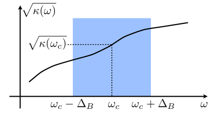
Figure 11: (color online). Schematic illustration of the hierarchy of frequency scales assumed for the derivation of the quantum Master equation. Following the standard treatment yamamoto99 , the reservoir spectral density $\kappa\left(\omega\right)/2\pi$ is taken to be a flat function of $\omega$ within the frequency range of interest $\left[\omega_{c}-\Delta_{B},\omega_{c}+\Delta_{B}\right]$.

We consider a generic linear coupling between the resonator mode and a set of independent harmonic oscillators (representing e.g. the modes of the free electromagnetic field), as described by the following textbook system-bath Hamiltonian

$$H = \underset{=H_{0}}{\underbrace{H_{S}+H_{B}}}+H_{I},$$ (114)

$$H_{S} = \omega_{c}a^{\dagger}a+g\mathcal{S}\otimes\left(a+a^{\dagger}\right),$$ (115)

$$H_{B} = \int_{\omega_{c}-\Delta_{B}}^{\omega_{c}+\Delta_{B}}d\omega\omega b_{\omega}^{\dagger}b_{\omega},$$ (116)

$$H_{I} = \int_{\omega_{c}-\Delta_{B}}^{\omega_{c}+\Delta_{B}}d\omega\sqrt{\frac{\kappa\left(\omega\right)}{2\pi}}\left(a^{\dagger}b_{\omega}+ab_{\omega}^{\dagger}\right),$$ (117)

where $b_{\omega}$ refer to bosonic bath operators obeying standard commutation relations with $[b_{\omega},b_{\omega^{\prime}}^{\dagger}]=\delta\left(\omega-\omega^{\prime}\right)$ etc. and $\Delta_{B}$ denotes the characteristic bandwidth of the bath zollerOnline ; rable14-lecture ; guimond16 . Within a rotating-wave approximation, we have dropped all energy non-conserving terms, which is valid if the system’s characteristic frequency $\omega_{c}$ is the largest frequency in the problem rable14-lecture . The bandwidth $\Delta_{B}$ is the frequency range over which the system-bath coupling is valid; it is closely related to the characteristic memory or correlation time of the bath $\tau_{c}\sim\Delta_{B}^{-1}$, as can be readily seen from the relation

$$\int_{\omega_{c}-\Delta_{B}}^{\omega_{c}+\Delta_{B}}d\omega e^{-i\omega\tau} = 2\Delta_{B}e^{-i\omega_{c}\tau}\mathrm{sinc}\left(\Delta_{B}\tau\right)$$ (118)

$$= 2\pi\delta_{\Delta_{B}}\left(\tau\right)e^{-i\omega_{c}\tau},$$ (119)

as it appears in the standard derivation of the Master equation presented below (if the spectral noise density $\kappa\left(\omega\right)$ and the thermal occupation number $\bar{n}_{\mathrm{th}}\left(\omega\right)$ are evaluated self-consistently at $\omega=\omega_{c}$). Here, the function $\delta_{\Delta_{B}}\left(\tau\right)=\pi^{-1}\Delta_{B}\mathrm{sinc}\left(\Delta_{B}\tau\right)$ is a well-known diffraction-like function with a maximal amplitude $\Delta_{B}/\pi$ at $\tau=0$ and a width of the order of $\tau_{c}\sim 2\pi/\Delta_{B}$ cohen92 . Since the integral equals one, this function is an approximate delta function which tends to $\delta\left(\tau\right)$ in the so-called white-noise limit $\Delta_{B}\rightarrow\infty$ (that is, $\tau_{c}\rightarrow 0$). Intuitively, $\delta_{\Delta_{B}}\left(\tau\right)$ can be seen as a slowly-varying function (on the $\sim\omega_{c}^{-1}$ timescale) that effectively acts as a delta function on timescales of the system evolution (i.e., much slower than $1/\Delta_{B}$). Typically, $\Delta_{B}\ll\omega_{c}$ is assumed zollerOnline ; rable14-lecture , but $\tau_{c}$ is still much shorter than the relevant timescales of the system dynamics $\tau_{\mathrm{sys}}$ (other than the free rotation $\omega_{c}$), that is

$$\omega_{c}\gg\Delta_{B}\gg\tau_{\mathrm{sys}}^{-1}.$$ (120)

In this case, the bandwidth $\Delta_{B}$ can be much larger than the spin-resonator coupling strength $g$ (which implies $g\tau_{c}\ll 1$, as required for the standard master equation treatment discussed below), but still much smaller than the characteristic frequency $\omega_{c}$. The system-reservoir coupling is usually only valid within a bandwidth $2\Delta_{B}\ll\omega_{c}$ around $\omega_{c}$ rable14-lecture . Within this frequency range the coupling strength may be approximated by a constant value as $\kappa\left(\omega\right)\approx\kappa\left(\omega_{c}\right)$, as schematically depicted in Fig.11.

J.2 Microscopic Derivation of the Master Equation

Our analysis is based on the standard Born-Markov framework, where correlations between the system and the bath are neglected (on relevant timescales), since the bath is considered to be very large and the effect of the interaction with the (small) system is negligible. Within this standard Born-Markov approximation gardiner00 ; cohen92 , in the interaction picture the system’s dynamics are described by

$$\dot{\tilde{\rho}}=-\int_{0}^{\infty}d\tau\mathrm{Tr}_{B}\left\{\left[\tilde{H}_{I}\left(t\right),\left[\tilde{H}_{I}\left(t-\tau\right),\tilde{\rho}\left(t\right)\rho_{B}\right]\right]\right\},$$ (121)

with $\tilde{\rho}=e^{iH_{0}t}\rho\left(t\right)e^{-iH_{0}t}$, $\tilde{H}_{I}\left(t\right)=e^{iH_{0}t}H_{I}e^{-iH_{0}t}$ and $\rho_{B}=Z^{-1}\exp\left[-\beta H_{B}\right]$ refers to a thermal state of the bath with the standard thermal correlations functions gardiner00

$$\mathrm{Tr}_{B}\left[b_{\omega}^{\dagger}b_{\omega^{\prime}}\rho_{B}\right]=\bar{n}_{\mathrm{th}}\left(\omega\right)\delta\left(\omega-\omega^{\prime}\right),$$ (122)

etc. Eq.(121) can equivalently be expressed as

$$\dot{\tilde{\rho}} = \int_{0}^{\infty}d\tau\mathrm{Tr}_{B}\{\underset{\leavevmode\hbox to14.18pt{\vbox to14.18pt{\text{[drawing]}}}}{\underbrace{\tilde{H}_{I}\left(t\right)\tilde{\rho}\left(t\right)\rho_{B}\tilde{H}_{I}\left(t-\tau\right)}}-\tilde{H}_{I}\left(t\right)\tilde{H}_{I}\left(t-\tau\right)\tilde{\rho}\left(t\right)\rho_{B}+\mathrm{h.c.}\}$$ (123)

In the interaction picture, the system-bath coupling reads explicitly

$$\tilde{H}_{I}\left(t\right)=\int_{\omega_{c}-\Delta_{B}}^{\omega_{c}+\Delta_{B}}d\omega\sqrt{\frac{\kappa\left(\omega\right)}{2\pi}}\left\{e^{-i\omega t}b_{\omega}\left[e^{i\omega_{c}t}\left(a^{\dagger}+\mu\mathcal{S}\right)-\mu\mathcal{S}\right]+e^{i\omega t}b_{\omega}^{\dagger}\left[e^{-i\omega_{c}t}\left(a+\mu\mathcal{S}\right)-\mu\mathcal{S}\right]\right\},$$ (124)

where we have used the fact that the resonator annihilation operators transform as

$$\tilde{a}\left(t\right)=e^{iH_{S}t}ae^{-iH_{S}t}=e^{-i\omega_{c}t}\left(a+\mu\mathcal{S}\right)-\mu\mathcal{S},$$ (125)

while the bath operators transform simply as $\tilde{b}_{\omega}\left(t\right)=e^{iH_{B}t}b_{\omega}e^{-iH_{B}t}=e^{-i\omega t}b_{\omega}$. Next, let us single out one term explicitly, but all other terms follow analogously. Using the thermal correlation functions as stated in Eq.(122), we then obtain

$$\mathrm{Tr}_{B}\left\{\leavevmode\hbox to14.18pt{\vbox to14.18pt{\text{[drawing]}}}\right\} = \int_{\omega_{c}-\Delta_{B}}^{\omega_{c}+\Delta_{B}}d\omega\frac{\kappa\left(\omega\right)}{2\pi}\bar{n}_{\mathrm{th}}\left(\omega\right)e^{-i\omega\tau}\left[e^{i\omega_{c}t}\left(a^{\dagger}+\mu\mathcal{S}\right)-\mu\mathcal{S}\right]\tilde{\rho}\left(t\right)\left[e^{-i\omega_{c}\left(t-\tau\right)}\left(a+\mu\mathcal{S}\right)-\mu\mathcal{S}\right]$$ (126)

$$+\int_{\omega_{c}-\Delta_{B}}^{\omega_{c}+\Delta_{B}}d\omega\frac{\kappa\left(\omega\right)}{2\pi}\left[\bar{n}_{\mathrm{th}}\left(\omega\right)+1\right]e^{i\omega\tau}\left[e^{-i\omega_{c}t}\left(a+\mu\mathcal{S}\right)-\mu\mathcal{S}\right]\tilde{\rho}\left(t\right)\left[e^{i\omega_{c}\left(t-\tau\right)}\left(a^{\dagger}+\mu\mathcal{S}\right)-\mu\mathcal{S}\right],$$

and similar expressions for the remaining terms in Eq.(121). In the next step, we perform the integration over the past, using the relation carmichael02

$$\int_{0}^{\infty}d\tau e^{\pm i\left(\omega_{c}-\omega\right)\tau}=\pi\delta\left(\omega_{c}-\omega\right)\pm i\mathbb{P}\frac{1}{\omega_{c}-\omega},$$ (127)

with $\mathbb{P}$ denoting Cauchy’s principal value, perform the integration over frequency, and within a rotating wave approximation (which is valid for the realistic parameter regime $\mu\kappa\left(\omega_{c}\right)\bar{n}_{\mathrm{th}}\left(\omega_{c}\right)\sqrt{\bar{n}_{\mathrm{th}}\left(\omega_{c}\right)}\ll\omega_{c}$) drop all fast oscillating terms $\sim\exp\left[\pm i\omega_{c}t\right]$. After some simple manipulations, we then arrive at the master equation

$$\dot{\tilde{\rho}} = \kappa\left(\omega_{c}\right)\left[\bar{n}_{\mathrm{th}}\left(\omega_{c}\right)+1\right]\mathcal{D}\left[a+\mu\mathcal{S}\right]\tilde{\rho}$$ (128)

$$+\kappa\left(\omega_{c}\right)\bar{n}_{\mathrm{th}}\left(\omega_{c}\right)\mathcal{D}\left[a^{\dagger}+\mu\mathcal{S}\right]\tilde{\rho}$$

$$-i\Delta_{c}\left[\left(a^{\dagger}+\mu\mathcal{S}\right)\left(a+\mu\mathcal{S}\right),\tilde{\rho}\right]$$

$$+\gamma\mathcal{D}\left[\mathcal{S}\right]\tilde{\rho}-i\Delta_{S}\left[\mathcal{S}^{2},\tilde{\rho}\right].$$

Here, we have introduced the decay rate

$$\gamma = \mu^{2}\int_{\omega_{c}-\Delta_{B}}^{\omega_{c}+\Delta_{B}}d\omega\kappa\left(\omega\right)\left[2\bar{n}_{\mathrm{th}}\left(\omega\right)+1\right]\delta\left(\omega-0\right),$$ (129)

which derives from the terms in Eq.(126) rotating at zero frequency, and the Lamb-like energy shifts

$$\Delta_{c} = \mathbb{P}\int_{\omega_{c}-\Delta_{B}}^{\omega_{c}+\Delta_{B}}d\omega\frac{\kappa\left(\omega\right)}{2\pi}\frac{1}{\omega_{c}-\omega},$$ (130)

$$\Delta_{S} = \mu^{2}\mathbb{P}\int_{\omega_{c}-\Delta_{B}}^{\omega_{c}+\Delta_{B}}d\omega\frac{\kappa\left(\omega\right)}{2\pi}\frac{1}{\omega}.$$ (131)

In accordance with the frequency regime $\left(\omega_{c}\gg\Delta_{B}\gg\tau_{\mathrm{sys}}^{-1}\right)$ discussed above, we assume the bandwidth $\Delta_{B}$ to be large, but finite. In this case, the rate $\gamma$ vanishes $\left(\gamma=0\right)$, as the integration range does not cover the $\delta$-peak at $\omega=0$. Physically, the regime where the lower limit of the relevant frequency range $\omega_{c}-\Delta_{B}$ does not extend all the way down to zero frequency amounts to the existence of a lower frequency cut-off $\omega_{\mathrm{cut}}=\omega_{c}-\Delta_{B}$. For example, such a lower frequency cut-off $\omega_{\mathrm{cut}}$ naturally arises in the context of a phonon bath where the existence of $\omega_{\mathrm{cut}}\sim\lambda_{\mathrm{cut}}^{-1}$ is due to finite device dimensions (since a phonon wavelength $\lambda$ larger than the device dimensions is not supported by this structure). Moreover, phonons with a wavelength much larger than the resonator are not able to resolve the resonator and simply represent a global shift of the resonator structure as a whole (and therefore do not linearly couple to the localized resonator mode). On the contrary, in the limit of infinite bandwidth $\Delta_{B}\rightarrow\infty$, the decay rate $\gamma$ (as well as the Lamb-like shifts $\Delta_{c},\Delta_{S}$) will depend on the relevant reservoir spectral density

$$\kappa\left(\omega\right)/2\pi=g^{2}\left(\omega\right)D_{\mathrm{DOS}}\left(\omega\right),$$ (132)

often abbreviated as $J\left(\omega\right)=\kappa\left(\omega\right)/2\pi$ in the literature deVega15 . The spectral density $J\left(\omega\right)=\sum_{k}\left|g_{k}\right|^{2}\delta\left(\omega-\omega_{k}\right)$ encodes the features of the environment relevant for the reduced system description, and depends on both the environmental density of the modes $D_{\mathrm{DOS}}\left(\omega\right)$ and on how strongly the system couples to each mode $\sim g\left(\omega\right)$. For concreteness, let us discuss two particular examples: (i) First, in quantum optical systems typically $J\left(\omega\right)\sim\omega^{n}$ for a positive integer $n$ yamamoto99 ; carmichael02 ; in particular, for coupling of a harmonic oscillator to the electromagnetic field in three dimensions in free space the spectral density scales as $J\left(\omega\right)\sim\omega^{3}$ paavola08 . In this case, even in the absence of a lower frequency cut-off $\omega_{\mathrm{cut}}$, the rate $\gamma$ vanishes, because $\kappa\left(\omega\right)\bar{n}_{\mathrm{th}}\left(\omega\right)\sim\omega^{2}\rightarrow 0$ in the limit $\omega\rightarrow 0$. (ii) Second, a prominent phenomenological ansatz frequently used in the literature is the so-called Caldeira-Leggett model, where $J\left(\omega\right)\sim\omega^{\alpha}\Omega_{\mathrm{cut}}^{1-\alpha}e^{-\omega/\Omega_{\mathrm{cut}}}$ for all $\alpha>0$ and some high-frequency cut-off $\Omega_{\mathrm{cut}}$ deVega15 . Environments with $0<\alpha<1$ are referred to as sub-ohmic, while those corresponding to $\alpha=1$ and $\alpha>1$ are called ohmic and super-ohmic, respectively deVega15 . Within this Caldeira-Leggett model (and for $\Delta_{B}\rightarrow\infty$), the decay rate $\gamma$ given in Eq.(129) vanishes for super-ohmic spectral densities with $\alpha>1$, becomes a constant for $\alpha=1$ and diverges for $\alpha<1$, since $\bar{n}_{\mathrm{th}}\left(\omega\right)\sim k_{B}T/\omega$ for $k_{B}T\gg\omega$.

Here, we restrict our analysis to the regime where $\gamma$ vanishes, either because of the existence of a lower frequency cut-off $\omega_{\mathrm{cut}}>0$ or a spectral density with $J\left(\omega\right)\sim\omega^{\alpha}\left(\alpha>1\right)$, as discussed above. Moreover, following the standard treatment beaudoin11 ; cohen92 we neglect the Lamb shift $\Delta_{S}\sim\mu^{2}$ (typically, it is assumed that the Cauchy principal part of an integral of the spectral density is very small compared to the real part expressions gardiner00 ; scala07 ), yielding the master equation

$$\dot{\tilde{\rho}} = \kappa\left(\omega_{c}\right)\left[\bar{n}_{\mathrm{th}}\left(\omega_{c}\right)+1\right]\mathcal{D}\left[a+\mu\mathcal{S}\right]\tilde{\rho}$$ (133)

$$+\kappa\left(\omega_{c}\right)\bar{n}_{\mathrm{th}}\left(\omega_{c}\right)\mathcal{D}\left[a^{\dagger}+\mu\mathcal{S}\right]\tilde{\rho}$$

$$-i\Delta_{c}\left[\left(a^{\dagger}+\mu\mathcal{S}\right)\left(a+\mu\mathcal{S}\right),\tilde{\rho}\right],$$

which (due to the interaction-mediated hybridization of spin and resonator degrees of freedom $\sim g$) displays correlated decay terms of both resonator and spin degrees of freedom, that are proportional to the effective rate $\sim\kappa\left(\omega\right)\bar{n}_{\mathrm{th}}\left(\omega\right)$ evaluated at the (large) characteristic system frequency $\omega_{c}$. Using the relation

$$e^{-iH_{S}t}\left(a+\mu\mathcal{S}\right)e^{iH_{S}t}=e^{i\omega_{c}t}\left(a+\mu\mathcal{S}\right),$$ (134)

the corresponding master equation in the Schrödinger picture is found to be

$$\dot{\rho} = \kappa\left(\omega_{c}\right)\left[\bar{n}_{\mathrm{th}}\left(\omega_{c}\right)+1\right]\mathcal{D}\left[a+\mu\mathcal{S}\right]\rho$$ (135)

$$+\kappa\left(\omega_{c}\right)\bar{n}_{\mathrm{th}}\left(\omega_{c}\right)\mathcal{D}\left[a^{\dagger}+\mu\mathcal{S}\right]\rho$$

$$-i\left[H_{S},\rho\right]-i\Delta_{c}\left[\left(a^{\dagger}+\mu\mathcal{S}\right)\left(a+\mu\mathcal{S}\right),\rho\right].$$

In what follows, we restrict our analysis to the experimentally most relevant regime of weak spin-resonator coupling where $\mu=g/\omega_{c}\ll 1$. Within the corresponding approximation of independent rates of variation cohen92 , the interactions with the environment are treated separately for spin and resonator degrees of freedom; in other words, they can approximately treated as independent entities and the terms (rates of variation) due to internal and dissipative dynamics are added independently. While for ultra-strong coupling the qubit-resonator system needs to be treated as a whole when studying its interaction with the environment beaudoin11 , yielding irreversible dynamics through jumps between dressed states (rather than bare states), in the weak coupling regime we recover standard (quantum optical) dissipators, i.e.,

$$\dot{\rho} = -i\left[H_{S},\rho\right]+\kappa\left[\bar{n}_{\mathrm{th}}+1\right]\mathcal{D}\left[a\right]\rho+\kappa\bar{n}_{\mathrm{th}}\mathcal{D}\left[a^{\dagger}\right]\rho.$$ (136)

In the last step, we have set $\kappa\equiv\kappa\left(\omega_{c}\right)$, $\bar{n}_{\mathrm{th}}\equiv\bar{n}_{\mathrm{th}}\left(\omega_{c}\right)$ and dropped the energy shift $\Delta_{c}$ which may be incorporated into a renormalized cavity frequency $\omega_{c}\rightarrow\omega_{c}+\Delta_{c}$.

$\kappa/\omega_{c}\bar{n}_{\mathrm{th}}\left[10^{-3}\right]$	0	0.5	1	1.5	2	2.5
$\xi_{\kappa}\left[\%\right]$ for uncorrelated noise	0.0	0.21	0.41	0.61	0.81	1.01
$\xi_{\kappa}\left[\%\right]$ for correlated noise	0.0	0.10	0.20	0.30	0.40	0.50

Table 1: Comparison of the rethermalization-induced error $\xi_{\kappa}\left[\%\right]$ for two different master equations, namely Eq.(136) (uncorrelated noise model) and $\dot{\rho}=-i\left[H_{S},\rho\right]+\kappa\left[\bar{n}_{\mathrm{th}}+1\right]\mathcal{D}\left[a+\mu\mathcal{S}\right]\rho+\kappa\bar{n}_{\mathrm{th}}\mathcal{D}\left[a^{\dagger}+\mu\mathcal{S}\right]\rho$ (correlated noise model). The error found for the uncorrelated noise model (as used in the main text) is about twice as large as the one found for the correlated one, and may therefore be seen as a conservative estimate. Note that Fig.4(c) of the main text is partially based on the first row (uncorrelated noise model). Other numerical parameters: $\mu=g/\omega_{c}=1/16$, $\Gamma=0$, $k_{B}T/\omega_{c}=2$ and $\omega_{q}=0$.

Note that the approximate replacement of the correlated dissipators by uncorrelated ones, that is $\mathcal{D}\left[a+\mu\mathcal{S}\right]\rho\rightarrow\mathcal{D}\left[a\right]\rho$ and $\mathcal{D}\left[a^{\dagger}+\mu\mathcal{S}\right]\rho\rightarrow\mathcal{D}\left[a^{\dagger}\right]\rho$, gives rise to a conservative error estimate for our hot gate. As can be shown analytically (compare Appendix L), the rethermalization-induced error $\xi_{\kappa}$ induced by independent decay terms as given in Eq.(136) is twice as large as the one due to correlated decay terms. This statement has also been verified numerically; compare Tab.1.

While Eq.(136) is not rigorous (given the approximations made throughout its derivation), this type of noise model (with independent rather than correlated decay terms, and complemented by additional dissipators for the qubits) has been used widely to describe a great variety of relevant spin-resonator systems (in the regime of weak spin-resonator coupling for values up to $\mu=g/\omega_{c}\lesssim 4\%$ blais07 ), ranging e.g. from superconducting qubits blais04 ; blais07 as well as quantum dots coupled to transmission line resonators gullans15 ; liu14 , to NV-center spins rabl09 or carbon nanotubes wang15 coupled to nanomechanical oscillators. For example, in Refs.gullans15 ; liu14 very good agreement with experimental results has been achieved for $\mu\sim 1\%$.

We conclude this discussion with a final remark on low-frequency noise: As shown above, the existence of a low-frequency cut-off does exclude low-frequency contributions to resonator-mediated dephasing of the spins (since $\gamma=0$). Still, low-frequency noise (deriving for example from ambient nuclear spins hanson08 ) may still couple directly to the qubits. In our model, this type of noise is captured by the dephasing rate $\Gamma$, which may, however, be mitigated efficiently by simple spin-echo techniques.

Appendix K Additional Numerical Results

Here, we provide further detailed results based on the numerical simulation of the master equation given in Eq.(7). Just as in the main text, for all simulations shown below the initial state of the spin-resonator system has been chosen as $\rho\left(0\right)=\left|\Uparrow\Downarrow\right\rangle\left\langle\Uparrow\Downarrow\right|\otimes\rho_{\mathrm{th}}\left(T\right)$, with the cavity mode in the thermal state $\rho_{\mathrm{th}}\left(T\right)=Z^{-1}\exp\left[-\beta\omega_{c}a^{\dagger}a\right]$. Apart from the state fidelity $\mathcal{F}$,we also quantify the logarithmic negativity $E_{\mathcal{N}}$ (which ranges between $0$ for separable states to at maximum $1$ for two maximally-entangled qubits) in order to quantify the entanglement between the two qubits.

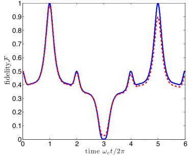
Figure 12: (color online). Fidelity $\mathcal{F}$ for the two-qubit state $\rho_{\mathrm{qubits}}$ with the target state $\left|\Psi_{\mathrm{tar}}\right\rangle=\left(\left|\Uparrow\Downarrow\right\rangle+i\left|\Downarrow\Uparrow\right\rangle\right)/\sqrt{2}$ for $\Gamma/\omega_{c}=0$ (blue solid line) and $\Gamma/\omega_{c}=1\%$ (red dashed line). For sufficiently low noise, at $\omega_{c}t=2\pi$ and $\omega_{c}t=5\times 2\pi$ the fidelity with the maximally entangled state $\left|\Psi_{\mathrm{tar}}\right\rangle$ reaches the maximal value $\mathcal{F}=1$. Numerical parameters: $\omega_{q}/\omega_{c}=0$, $k_{B}T/\omega_{c}=2$ $\left(\bar{n}_{\mathrm{th}}\approx 1.54\right)$, $g/\omega_{c}=1/4$, $\kappa/\omega_{c}=Q^{-1}=10^{-5}$.

Periodic recurrences.—First, as displayed in Fig.12, we observe periodic recurrences of the maximally-entangling dynamics: For example, for $g/\omega_{c}=1/4$ (as used in Fig.12), ideally—apart from $\mathcal{F}=1$ at $(\omega_{c}/2\pi)t=1$—we find $\mathcal{F}=1$ again at $(\omega_{c}/2\pi)t=5$, since $U_{\mathrm{id}}^{x}\left(m=5,1/4\right)=\exp\left[i\pi\sigma_{1}^{x}\sigma_{2}^{x}\right]U_{\mathrm{id}}^{x}\left(1,1/4\right)=-U_{\mathrm{id}}^{x}\left(1,1/4\right)$. This statement holds provided that dephasing is negligible on the relevant timescale; compare the dashed curve in Fig.12 which accounts for dephasing of the qubits.

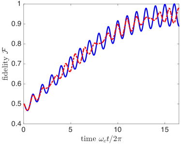
Figure 13: (color online). Fidelity $\mathcal{F}=\left<\Psi_{\mathrm{tar}}|\rho_{\mathrm{qubits}}|\Psi_{\mathrm{tar}}\right>$ for the two-qubit state $\rho_{\mathrm{qubits}}=\mathrm{Tr}_{\mathrm{cav}}\left[\rho\right]$ with the target state $\left|\Psi_{\mathrm{tar}}\right\rangle=\left(\left|\Uparrow\Downarrow\right\rangle+i\left|\Downarrow\Uparrow\right\rangle\right)/\sqrt{2}$ for both $\omega_{q}/\omega_{c}=0$ (solid blue line) and $\omega_{q}/\omega_{c}=0.1$ (dashed red line); here, $g/\omega_{c}=1/16<0.1$. Other numerical parameters: $k_{B}T/\omega_{c}=2$ $(\bar{n}_{\mathrm{th}}\approx 1.54)$, $Q=10^{5}$ and $\Gamma/\omega_{c}=0$.

Figure 14: (color online). Logarithmic negativity $E_{\mathcal{N}}$ for $k_{B}T/\omega_{c}=1$ and different cavity quality factors: $Q=10^{5}$ (solid blue), $Q=10^{2}$ (dash-dotted blue), and $Q=10$ (dashed magenta). A clear reduction of the maximum entanglement is observed, if the quality factor $Q$ is too low to satisfy the hot-gate requirement given in Eq.(8). Here, we have $g/\omega_{c}\times g/k_{B}T=1/16=6.25\times 10^{-2}$. The red (dotted) curve refers to $Q=10^{2}$ and $\omega_{q}/\omega_{c}=0.2$. Other numerical parameters: $g/\omega_{c}=1/4$ and $\Gamma/\omega_{c}=0$.

Non-zero level splitting.—While our analytical treatment has assumed $\omega_{q}=0$, in Fig.13 we provide exemplary numerical results that explicitly account for a non-zero qubit level splitting $\omega_{q}>0$, showing that the proposed protocol can tolerate non-zero level splittings of the qubits $\omega_{q}/\omega_{c}\lesssim 0.1$, without a severe reduction in the fidelity of the protocol. Again, this numerical finding is corroborated in Fig.14. Here, it is shown explicitly that a strong entanglement reduction is observed once condition (8) is violated. Conversely, within the range of parameter values satisfying Eq.(8), the results are rather insensitive to the particular parameter values.

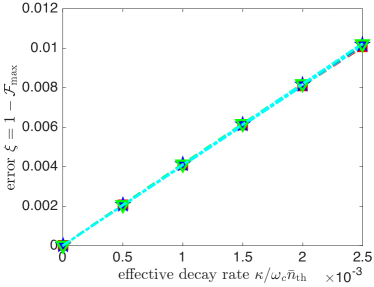
Figure 15: (color online). Error as a function of the effective rethermalization rate $\kappa\bar{n}_{\mathrm{th}}$ for $g/\omega_{c}=1/16$ (red squares), $g/\omega_{c}=1/\left(8\sqrt{2}\right)$ (blue stars) and $g/\omega_{c}=1/8$ (green triangles) and $k_{B}T/\omega_{c}=2$ $\left(\bar{n}_{\mathrm{th}}\approx 1.54\right)$, within the relevant small-error regime ($\kappa_{\mathrm{eff}}/g_{\mathrm{eff}}\ll 1$). The dash-dotted lines in cyan refer to linear fits, demonstrating a linear error scaling in the small error-regime ($\kappa_{\mathrm{eff}}/g_{\mathrm{eff}}\ll 1$), which is independent of $\mu=g/\omega_{c}$. Accordingly, the error is larger for higher temperatures, but all temperature related effects are approximately captured by the thermal occupation number $\bar{n}_{\mathrm{th}}$. Other numerical parameters: $\Gamma=0$ and $\omega_{q}=0$.

Rethermalization-induced errors.—As illustrated in Fig.15, we have numerically checked that (for small infidelities) the rethermalization induced error $\xi_{\kappa}$ scales linearly with the effective rethermalization rate $\kappa_{\mathrm{eff}}=\kappa\bar{n}_{\mathrm{th}}$. Notably, as evidenced in Fig.15, the error is found to be independent of the spin-resonator coupling $g$. As demonstrated in in Sec. L, this numerical result can be corroborated analytically within a perturbative framework.

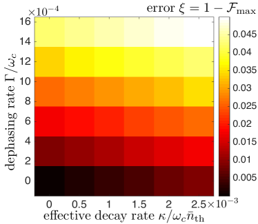
Figure 16: (color online). Total error $\xi$ as a function of both the effective rethermalization rate $\sim\kappa/\omega_{c}\bar{n}_{\mathrm{th}}\sim\bar{n}_{\mathrm{th}}/Q$ and the spin dephasing rate $\sim\Gamma/\omega_{c}$ for $g/\omega_{c}=1/16$, $k_{B}T/\omega_{c}=4$ and $\omega_{q}=0$.

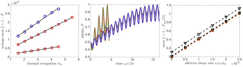
Figure 17: (color online). Timing errors. Left: Total average error $\bar{\xi}$ as a function of the thermal occupation number $\bar{n}_{\mathrm{th}}$ for timing windows $\left(\omega_{c}/2\pi\right)\Delta t=5\%$ (circles) and $\left(\omega_{c}/2\pi\right)\Delta t=10\%$ (squares); here, $g/\omega_{c}=1/16$ (red symbols) and $g/\omega_{c}=1/8$ (blue symbols, upper curve). All curves can be fit very well to linear error models (see black dashed lines). Center: Set of underlying (temperature-dependent) simulations for both $g/\omega_{c}=1/16$ (terminating at $\omega_{c}t/2\pi=16.5$) and $g/\omega_{c}=1/8$ (terminating at $\omega_{c}t/2\pi=4.5$). Note that larger amplitudes are observed for larger values of $\mu=g/\omega_{c}$. Other numerical parameters: $Q=10^{5}$, $\Gamma=0$ and $\omega_{q}=0$. Right: Same analysis as done in Fig.15 for $g/\omega_{c}=1/8$ (triangles) and $g/\omega_{c}=1/16$ (squares). The black curves account for a finite timing accuracy $\left(\omega_{c}/2\pi\right)\Delta t=5\%$, showing that the detrimental effects of time jitter are less pronounced for smaller values of $\mu=g/\omega_{c}$.

Full error analysis.—Similar to Fig.4(c) in the main text, in Fig.16 we provide numerical results that fully account for higher-order, correlated errors (beyond the linear error approximation). Here, we have chosen a temperature $k_{B}T/\omega_{c}=4$, a factor two larger than the one used in Fig.4(c) in the main text. Still, if the rethermalization induced error is scaled in terms of the effective decay rate $\kappa_{\mathrm{eff}}=\kappa\bar{n}_{\mathrm{th}}$, we obtain (approximately) the same total error $\xi$, independently of the temperature $k_{B}T$, showing that the effective decay rate $\kappa_{\mathrm{eff}}=\kappa\bar{n}_{\mathrm{th}}$ captures well any temperature-related effects. This is evidenced numerically in Fig.16 which approximately coincides with the results displayed in Fig.4(c) in the main text and is line with our simple error estimate for rethermalization induced errors; compare Eq.(10) in the main text.

Timing errors.—Finally, we consider errors (infidelities) due to limited timing accuracies. To do so, we take the average fidelity of our protocol $\bar{\mathcal{F}}$ within a certain timing window $\Delta t$ centered around the stroboscopic time $t_{\mathrm{max}}$ for which maximum fidelity (minimal infidelity) is achieved; for example, in quantum dot systems timing accuracies $\Delta t$ of a few picoseconds have been demonstrated experimentally bocquillon13-sm . For $g/2\pi=10\mathrm{MHz}$ and $\omega_{c}/2\pi=160\mathrm{MHz}$ (that is, $\mu=g/\omega_{c}=1/16$) as used in the main text, the pulse time lies in the microsecond regime $\left(t_{\mathrm{max}}=\pi/8g_{\mathrm{eff}}\approx 0.2\mu\mathrm{s}\right)$, for which $\Delta t\approx 1\mathrm{ps}$ is feasible; for this relatively long pulse, the relative time jitter is well below the percent level, i.e., $\left(\omega_{c}/2\pi\right)\Delta t\approx 10^{-4}$. Based on our numerical simulations, we make the following observations: (i) As demonstrated in Fig.17, we find an average error scaling linearly with $\sim\bar{n}_{\mathrm{th}}$, that is $\bar{\xi}=1-\bar{\mathcal{F}}\sim\bar{n}_{\mathrm{th}}$. (ii) More precisely, the error expressions given in the main text can be generalized to

$$\bar{\xi}=\bar{\alpha}_{\text{$\kappa$}}\frac{\kappa}{\omega_{c}}\bar{n}_{\mathrm{th}}+\bar{\alpha}_{\Gamma}\frac{\Gamma}{\omega_{c}}+\bar{\beta}_{\kappa}+\bar{\beta}_{\Gamma}.$$ (137)

Here, the unit-less quantities $\bar{\alpha}_{\gamma},\bar{\beta}_{\gamma}$ for $\gamma=\kappa,\Gamma$ depend on the timing window $\Delta t$. For example, for $g/\omega_{c}=1/16$ and $\left(\omega_{c}/2\pi\right)\Delta t=5\%$, we then extract $\bar{\alpha}_{\text{$\kappa$}}\approx 4.03$, $\bar{\beta}_{\kappa}\approx 2.2\times 10^{-4}$, $\bar{\alpha}_{\Gamma}\approx 24.22$ and $\bar{\beta}_{\Gamma}\approx 5.1\times 10^{-4}$. (iii) As shown in Fig.17, for the experimentally most relevant regime where $\left(\omega_{c}/2\pi\right)\Delta t\ll 1$ (such that the timing window covers a small range of the oscillations only), this error is found to decrease for a smaller spin-resonator coupling strength $g/\omega_{c}$, because larger values of $g/\omega_{c}$ imply larger oscillation amplitudes within the relevant range over which we have to average; compare the center and right plots in Fig.17. Therefore, for the experimentally most relevant regime where $\left(\omega_{c}/2\pi\right)\Delta t\ll 1$ and $g/\omega_{c}\lesssim 1/16$, the effects of time jitter should be negligible.

Appendix L Analytical Expression for Rethermalization-Induced Errors

In this Appendix we derive an analytical expression for rethermalization-induced errors. In particular we show that this expression is independent of the spin-resonator coupling strength $g$.

Our analysis starts out from the master equation

$$\dot{\rho}=-i\left[H,\rho\right]+\sum_{j=1,2}\mathcal{D}\left[L_{j}\right]\rho,$$ (138)

where the Hamiltonian $H=\omega_{c}a^{\dagger}a+g\mathcal{S}\otimes\left(a+a^{\dagger}\right)$ refers to the ideal (noise-free) dynamics and the jump-operators $L_{1}=\sqrt{\kappa_{1}}a$, $L_{2}=\sqrt{\kappa_{2}}a^{\dagger}$ with $\kappa_{1}=\kappa\left(\bar{n}_{\mathrm{th}}+1\right)$ and $\kappa_{2}=\kappa\bar{n}_{\mathrm{th}}$ describe rethermalization of the resonator mode with a rate $\kappa=\omega_{c}/Q$ that is enhanced by the thermal occupation number $\bar{n}_{\mathrm{th}}$. It is convenient to move to an interaction picture, defined by $\tilde{\rho}\left(t\right)=\exp\left[iHt\right]\rho\left(t\right)\exp\left[-iHt\right]$. In this interaction picture, the system’s dynamics is described by

$$\dot{\tilde{\rho}}=\sum_{j=1,2}\mathcal{D}\left[\tilde{L}_{j}\right]\tilde{\rho},$$ (139)

with time-dependent jump operators $\tilde{L}_{j}=\exp\left[iHt\right]L_{j}\exp\left[-iHt\right]$. Using the exact relation $\exp\left[-iHt\right]=U\exp\left[-i\omega_{c}ta^{\dagger}a\right]U^{\dagger}U_{\mathrm{sp}}\left(t\right)$, with the polaron transformation $U=\exp\left[\mu\mathcal{S}\left(a-a^{\dagger}\right)\right]$ and the pure spin (entangling) gate $U_{\mathrm{sp}}\left(t\right)=\exp\left[i\mu^{2}\omega_{c}t\mathcal{S}^{2}\right]$, the time-dependent jump operators $\tilde{L}_{j}$ take on a simple form

$$\tilde{L}_{1}\left(\tau\right) = \sqrt{\kappa_{1}}\left[e^{-i\omega_{c}\tau}a+\left(e^{-i\omega_{c}\tau}-1\right)\mu\mathcal{S}\right],$$

$$\tilde{L}_{2}\left(\tau\right) = \sqrt{\kappa_{2}}\left[e^{i\omega_{c}\tau}a^{\dagger}+\left(e^{i\omega_{c}\tau}-1\right)\mu\mathcal{S}\right].$$ (140)

The formal solution to Eq.(139) reads

$$\tilde{\rho}\left(t\right)=\tilde{\rho}\left(0\right)+\sum_{j}\int_{0}^{t}d\tau\mathcal{D}\left[\tilde{L}_{j}\left(\tau\right)\right]\tilde{\rho}\left(\tau\right),$$ (141)

where in the interaction picture the zeroth-order solution $\tilde{\rho}_{0}\left(t\right)=\tilde{\rho}\left(0\right)=\rho\left(0\right)$ stays inert, and accounts for the ideal (noise-free) dynamics only in the lab frame, $\rho_{0}\left(t\right)=\exp\left[-iHt\right]\tilde{\rho}_{0}\left(t\right)\exp\left[iHt\right]=\exp\left[-iHt\right]\rho\left(0\right)\exp\left[iHt\right]$. To obtain the first-order correction $\tilde{\rho}_{1}\left(t\right)$ within a perturbative framework, we re-insert the zeroth-order solution into the dissipator of Eq.(141), i.e. effectively we take $\tilde{\rho}\left(\tau\right)\rightarrow\rho\left(0\right)$, which yields $\tilde{\rho}\left(t\right)\approx\rho\left(0\right)+\tilde{\rho}_{1}\left(t\right)$, with

$$\tilde{\rho}_{1}\left(t\right)=\sum_{j}\int_{0}^{t}d\tau\mathcal{D}\left[\tilde{L}_{j}\left(\tau\right)\right]\rho\left(0\right).$$ (142)

Inserting the expressions given in Eq.(140) into Eq.(142) and performing the integration, with $\int_{0}^{t}d\tau\left|1-e^{\pm i\omega_{c}\tau}\right|^{2}=2(t-\frac{\sin\left(\omega_{c}t\right)}{\omega_{c}})$ and $\int_{0}^{t}d\tau\left(1-e^{\pm i\omega_{c}\tau}\right)=t\pm i\frac{e^{\pm i\omega_{c}t}-1}{\omega_{c}}$ , one arrives at

$$\tilde{\rho}_{1}\left(t\right) = \kappa_{1}t\mathcal{D}\left[a\right]\rho\left(0\right)+\kappa_{2}t\mathcal{D}\left[a^{\dagger}\right]\rho\left(0\right)+2\left(\kappa_{1}+\kappa_{2}\right)\mu^{2}\left(t-\frac{\sin\left(\omega_{c}t\right)}{\omega_{c}}\right)\mathcal{D}\left[\mathcal{S}\right]\rho\left(0\right)$$ (143)

$$+\left[\kappa_{1}\mu\left(t-i\frac{e^{-i\omega_{c}t}-1}{\omega_{c}}\right)\left\{a\rho\left(0\right)\mathcal{S}-\frac{1}{2}\left\{a\mathcal{S},\rho\left(0\right)\right\}\right\}+\mathrm{h.c.}\right]$$

$$+\left[\kappa_{2}\mu\left(t+i\frac{e^{i\omega_{c}t}-1}{\omega_{c}}\right)\left\{a^{\dagger}\rho\left(0\right)\mathcal{S}-\frac{1}{2}\left\{a^{\dagger}\mathcal{S},\rho\left(0\right)\right\}\right\}+\mathrm{h.c.}\right].$$

which, for stroboscopic times $t_{m}=2\pi m/\omega_{c}$ (with $m$ integer), simplifies to

$$\tilde{\rho}_{1}\left(t_{m}\right) = \kappa_{1}t_{m}\mathcal{D}\left[a\right]\rho\left(0\right)+\kappa_{2}t_{m}\mathcal{D}\left[a^{\dagger}\right]\rho\left(0\right)+2\left(\kappa_{1}+\kappa_{2}\right)\mu^{2}t_{m}\mathcal{D}\left[\mathcal{S}\right]\rho\left(0\right)$$

$$+\left[\kappa_{1}\mu t_{m}\left\{a\rho\left(0\right)\mathcal{S}-\frac{1}{2}\left\{a\mathcal{S},\rho\left(0\right)\right\}\right\}+\mathrm{h.c.}\right]+\left[\kappa_{2}\mu t_{m}\left\{a^{\dagger}\rho\left(0\right)\mathcal{S}-\frac{1}{2}\left\{a^{\dagger}\mathcal{S},\rho\left(0\right)\right\}\right\}+\mathrm{h.c.}\right].$$

Next, we perform a transformation back to the lab frame, with $\rho\left(t\right)=\exp\left[-iHt\right]\tilde{\rho}\left(t\right)\exp\left[iHt\right]$. As discussed in the main text, for stroboscopic times the ideal evolution simplifies to $\exp\left[-iHt_{m}\right]=\exp\left[i\mu^{2}2\pi m\mathcal{S}^{2}\right]=\exp\left(-i\phi_{\mathrm{gp}}\right)\exp\left[i4\pi m\mu^{2}\sigma_{1}^{x}\sigma_{2}^{x}\right]$. The ideal (noise-free) evolution is given by $\rho_{\mathrm{id}}\left(t_{m}\right)=\exp\left[-iHt_{m}\right]\rho\left(0\right)\exp\left[iHt_{m}\right]=\varrho_{\mathrm{id}}\left(t_{m}\right)\otimes\rho_{\mathrm{th}}$, where $\varrho_{\mathrm{id}}\left(t_{m}\right)=\exp\left[i4\pi m\mu^{2}\sigma_{1}^{x}\sigma_{2}^{x}\right]\varrho\left(0\right)\exp\left[-i4\pi m\mu^{2}\sigma_{1}^{x}\sigma_{2}^{x}\right]$ is the ideal qubit’s state at time $t_{m}$, starting from the initial state $\rho\left(0\right)=\varrho\left(0\right)\otimes\rho_{\mathrm{th}}$. Then, the system’s density matrix at time $t_{m}$ is approximately given by

$$\rho\left(t_{m}\right) = \rho_{\mathrm{id}}\left(t_{m}\right)+\kappa_{1}t_{m}\mathcal{D}\left[a\right]\rho_{\mathrm{id}}\left(t_{m}\right)$$

$$+\kappa_{2}t_{m}\mathcal{D}\left[a^{\dagger}\right]\rho_{\mathrm{id}}\left(t_{m}\right)$$

$$+2\left(\kappa_{1}+\kappa_{2}\right)\mu^{2}t_{m}\mathcal{D}\left[\mathcal{S}\right]\rho_{\mathrm{id}}\left(t_{m}\right)$$

$$+\left[\kappa_{1}\mu t_{m}\left\{a\rho_{\mathrm{id}}\left(t_{m}\right)\mathcal{S}-\frac{1}{2}\left\{a\mathcal{S},\rho_{\mathrm{id}}\left(t_{m}\right)\right\}\right\}\right.$$

$$\left.+\kappa_{2}\mu t_{m}\left\{a^{\dagger}\rho\left(0\right)\mathcal{S}-\frac{1}{2}\left\{a^{\dagger}\mathcal{S},\rho\left(0\right)\right\}\right\}+\mathrm{h.c.}\right].$$

Note that, in the limit $\kappa_{i}\rightarrow 0$, one retrieves the ideal result $\rho\left(t_{m}\right)=\rho_{\mathrm{id}}\left(t_{m}\right)$. Next, we trace out the resonator mode. Assuming the state of the resonator mode to be diagonal in the occupation number basis (in particular, this holds for a thermal state $\rho_{\mathrm{th}}$), none of the cross-terms contribute to the partial trace, and for stroboscopic times $t_{m}$ the state of the qubits is given by

$$\varrho\left(t_{m}\right)=\varrho_{\mathrm{id}}\left(t_{m}\right)+2\kappa\left(2\bar{n}_{\mathrm{th}}+1\right)t_{m}\mu^{2}\mathcal{D}\left[\mathcal{S}\right]\varrho_{\mathrm{id}}\left(t_{m}\right).$$ (144)

As expected naïvely, the error term scales with $\sim\kappa\bar{n}_{\mathrm{th}}t_{m}$, but it is further reduced by the factor $\mu^{2}=\left(g/\omega_{c}\right)^{2}$. Eq.(144) holds for stroboscopic times $t_{m}=2\pi m/\omega_{c}$, with $m$ integer. If $m\mu^{2}=1/16$, the ideal evolution $\exp\left[-iHt_{m}\right]=\exp\left(-i\phi_{\mathrm{gp}}\right)\exp\left[i\frac{\pi}{4}\sigma_{1}^{x}\sigma_{2}^{x}\right]$ equals a maximally-entangling gate, which (for an initial pure state like $\left|\Psi\right\rangle_{0}=\left|\Downarrow\Downarrow\right\rangle$) yields the desired ideal qubit target state $\left|\Psi_{\mathrm{tar}}\right\rangle=\exp\left[i\frac{\pi}{4}\sigma_{1}^{x}\sigma_{2}^{x}\right]\left|\Psi\right\rangle_{0}$. Then, in the presence of noise, at the nominally ideal time $t_{\mathrm{max}}=\pi/8\mu^{2}\omega_{c}=\pi/8g_{\mathrm{eff}}$ the qubit’s density matrix reads

$$\varrho\left(t_{\mathrm{max}}\right) = \left|\Psi_{\mathrm{tar}}\right\rangle\left\langle\Psi_{\mathrm{tar}}\right|$$

$$+\frac{\pi}{4}\frac{\kappa}{\omega_{c}}\left(2\bar{n}_{\mathrm{th}}+1\right)\mathcal{D}\left[\mathcal{S}\right]\left|\Psi_{\mathrm{tar}}\right\rangle\left\langle\Psi_{\mathrm{tar}}\right|.$$

Therefore, to first order rethermalization-induced noise leads to dephasing dynamics in the eigenbasis of $\mathcal{S}$ with a single such phase flip. Since neither the desired target state $\left|\Psi_{\mathrm{tar}}\right\rangle$ nor the initial state $\left|\Psi\right\rangle_{0}$ is an eigenstate of $\mathcal{S}$, the system looses fidelity with a probability $\frac{\pi}{4}\frac{\kappa}{\omega_{c}}\left(2\bar{n}_{\mathrm{th}}+1\right)$; notably, this expression is independent of the spin-resonator coupling strength $g$.

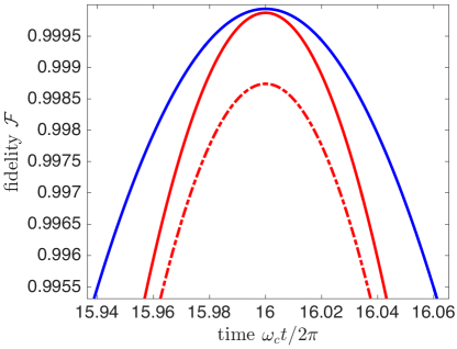
Figure 18: (color online). Fidelity $\mathcal{F}$ close to the ideal time $t_{\mathrm{max}}$ for $g/\omega_{c}=1/16$. The different curves refer to $Q=10^{5}$, $k_{B}T/\omega_{c}=2$, i.e. $\bar{n}_{\mathrm{th}}\approx 1.54$, (blue solid, top curve), $Q=10^{5}$, $k_{B}T/\omega_{c}=4$, i.e. $\bar{n}_{\mathrm{th}}\approx 3.52$, (red solid) and $Q=10^{4}$, $k_{B}T/\omega_{c}=4$ (red dash-dotted). The error $\xi=1-\mathcal{F}$ can be estimated well with the formula $\xi_{k}\approx 4\bar{n}_{\mathrm{th}}/Q$, giving (for example) $\mathcal{F}\approx 1-4\times 3.52/10^{4}\approx 0.9986$. Other numerical parameters: $\Gamma=0$ and $\omega_{q}=0$.

For the fidelity with the maximally entangled target state, we then obtain

$$\mathcal{F}=\left<\Psi_{\mathrm{tar}}|\varrho\left(t_{\mathrm{max}}\right)|\Psi_{\mathrm{tar}}\right>=1-\frac{\pi}{2}\frac{\kappa}{\omega_{c}}\left(2\bar{n}_{\mathrm{th}}+1\right),$$ (146)

with a thermalization-induced error term given by

$$\xi_{\kappa}=\pi\left(\kappa/\omega_{c}\right)\bar{n}_{\mathrm{th}}+\frac{\pi}{2}Q^{-1}.$$ (147)

This analytical result is in good agreement with our numerical findings (from which we have deduced $\xi_{\kappa}\approx\alpha_{\kappa}\left(\kappa/\omega_{c}\right)\bar{n}_{\mathrm{th}}$, with $\alpha_{\kappa}\approx 4$), showing (i) a linear scaling with the effective rethermalization rate $\sim\kappa\bar{n}_{\mathrm{th}}$, (ii) with a pre-factor $\alpha_{\kappa}=\pi$ (close to $\sim 4$) that is independent of the spin-resonator coupling strength $g$ and (iii) a constant offset $\sim Q^{-1}$ which is negligible for realistic quality factors $Q\approx 10^{5}-10^{6}$. The latter is due to photon/phonon emission with a rate $\sim\kappa=\omega_{c}/Q$ at $T\rightarrow 0$. As illustrated further in Fig.18 with a close-up of the fidelity $\mathcal{F}\left(t\right)$ around the optimal point $t_{\mathrm{max}}$, the error $\xi_{\kappa}$ can be estimated well with this simple formula, where all temperature related effects are captured by the simple linear expression in the thermal occupation number $\bar{n}_{\mathrm{th}}$.

Correlated noise model.—An analog analysis to the one presented above can be performed for a master equation with correlated (rather than uncorrelated) noise. In this case, as shown in Appendix J.2, the jump-operators are given by $L_{1}=\sqrt{\kappa_{1}}\left(a+\mu\mathcal{S}\right)$, $L_{2}=\sqrt{\kappa_{2}}\left(a^{\dagger}+\mu\mathcal{S}\right)$, which take on a simple form in the interaction picture, namely

$$\tilde{L}_{1}\left(\tau\right) = \sqrt{\kappa_{1}}e^{-i\omega_{c}\tau}\left(a+\mu\mathcal{S}\right),$$ (148)

$$\tilde{L}_{2}\left(\tau\right) = \sqrt{\kappa_{2}}e^{i\omega_{c}\tau}\left(a^{\dagger}+\mu\mathcal{S}\right),$$ (149)

as compared to Eq.(140) within the uncorrelated noise model discussed above. Then, following the same steps as above, the integration $\int_{0}^{t}d\tau\left|1-e^{\pm i\omega_{c}\tau}\right|^{2}=2(t-\frac{\sin\left(\omega_{c}t\right)}{\omega_{c}})$ is simply replaced by $\int_{0}^{t}d\tau=t$; accordingly, in this scenario, the pre-factor of the spin dephasing term $\mathcal{D}\left[\mathcal{S}\right]\rho\left(0\right)$ simplifies to $\sim\left(\kappa_{1}+\kappa_{2}\right)\mu^{2}t$, which for stroboscopic times $t_{m}=2\pi m/\omega_{c}$ is exactly a factor of two smaller than the corresponding rate in Eq.(143) for the uncorrelated noise model. In summary, along the lines of our previous analysis, for a correlated noise model Eqs.(144) and (147) should be replaced by

$$\varrho\left(t_{m}\right)=\varrho_{\mathrm{id}}\left(t_{m}\right)+\kappa\left(2\bar{n}_{\mathrm{th}}+1\right)t_{m}\mu^{2}\mathcal{D}\left[\mathcal{S}\right]\varrho_{\mathrm{id}}\left(t_{m}\right),$$ (150)

and

$$\xi_{\kappa}=\frac{\pi}{2}\left(\kappa/\omega_{c}\right)\bar{n}_{\mathrm{th}}+\frac{\pi}{4}Q^{-1},$$ (151)

respectively, showing that for uncorrelated spin-resonator noise the rethermalization-induced error is approximately twice as large as for correlated spin-resonator noise; also compare the numerical results presented in Tab. 1.

Appendix M Analytical Model for Dephasing-Induced Errors

In this Appendix we provide an analytical model for dephasing-induced errors. Neglecting rethermalization-induced errors for the moment, here we consider the following master equation

$$\dot{\rho}=\underset{\mathcal{L}_{0}\rho}{\underbrace{-i\left[H_{\mathrm{id}},\rho\right]}}+\underset{\mathcal{L}_{1}\rho}{\underbrace{\gamma_{\phi}\left[\mathcal{D}\left[\sigma_{1}^{z}\right]\rho+\mathcal{D}\left[\sigma_{2}^{z}\right]\rho\right]}},$$ (152)

where $H_{\mathrm{id}}=\omega_{c}a^{\dagger}a+g\left(\sigma_{1}^{z}+\sigma_{2}^{z}\right)\otimes\left(a+a^{\dagger}\right)$ describes the ideal (error-free), coherent evolution for longitudinal coupling between the qubits and the resonator mode, and $\gamma_{\phi}$ is the pure dephasing rate. Since the superoperators $\mathcal{L}_{0}$ and $\mathcal{L}_{1}$ as defined in Eq.(152) commute, that is $\left[\mathcal{L}_{0},\mathcal{L}_{1}\right]=0$ (since $\left[H_{\mathrm{id}},\mathcal{D}\left[\sigma_{i}^{z}\right]X\right]=\mathcal{D}\left[\sigma_{i}^{z}\right]\left[H_{\mathrm{id}},X\right]$ for any operator $X$), the full evolution simplifies to

$$\rho\left(t\right)=e^{\mathcal{L}_{1}t}e^{\mathcal{L}_{0}t}\rho\left(0\right)=e^{\mathcal{L}_{1}t}\rho_{\mathrm{id}}\left(t\right),$$ (153)

where we have defined the ideal target state at time $t$ as $\rho_{\mathrm{id}}\left(t\right)=\exp\left[\mathcal{L}_{0}t\right]\rho\left(0\right)$, which, starting from the initial state $\rho\left(0\right)$, exclusively accounts for the ideal (error-free), coherent evolution. For small infidelities $\left(\gamma_{\phi}t\ll 1\right)$, the deviation from the ideal dynamics $\Delta\rho=\rho-\rho_{\mathrm{id}}$ is approximately given by

$$\Delta\rho\left(t\right)\approx\gamma_{\phi}t\sum_{i}\mathcal{D}\left[\sigma_{i}^{z}\right]\rho_{\mathrm{id}}\left(t\right),$$ (154)

showing that (in the regime of interest where $\gamma_{\phi}t\ll 1$) the dominant dephasing induced errors are linearly proportional to $\sim\gamma_{\phi}t_{g}\sim\gamma_{\phi}/g_{\mathrm{eff}}=\gamma_{\phi}/\mu^{2}\omega_{c}$, as expected; here, $t_{g}\sim g_{\mathrm{eff}}$ is the relevant gate time which has to be short compared to $\gamma_{\phi}^{-1}$.

In what follows, for completeness we derive the same result within a quantum jump approach. Eq.(152) can be rewritten as

$$\dot{\rho} = -iH\rho+i\rho H^{\dagger}+\mathcal{J}\rho,$$ (155)

where $H=H_{\mathrm{id}}-i\gamma_{\phi}$ and $\mathcal{J}\rho=\gamma_{\phi}\sum_{i}\sigma_{i}^{z}\rho\sigma_{i}^{z}$. The formal solution to Eq.(155) reads

$$\rho\left(t\right)=e^{-iHt}\rho\left(0\right)e^{iH^{\dagger}t}+\int_{0}^{t}d\tau e^{-iH\left(t-\tau\right)}\mathcal{J}\rho\left(\tau\right)e^{iH^{\dagger}\left(t-\tau\right)}.$$ (156)

Defining the ideal target state at time $t$ as

$$\rho_{\mathrm{id}}\left(t\right)=e^{-iH_{\mathrm{id}}\left(t-\tau\right)}\rho\left(\tau\right)e^{iH_{\mathrm{id}}\left(t-\tau\right)},$$ (157)

the exact solution given in Eq.(156) can be iterated, giving an illustrative expansion in terms of the jumps $\mathcal{J}$. It reads

$$\rho\left(t\right) = \mathcal{U}\left(t\right)\rho\left(0\right)+\int_{0}^{t}d\tau_{1}\mathcal{U}\left(t-\tau_{1}\right)\mathcal{J}\mathcal{U}\left(\tau_{1}\right)\rho\left(0\right)$$

$$+\int_{0}^{t}d\tau_{2}\int_{0}^{\tau_{2}}d\tau_{1}\mathcal{U}\left(t-\tau_{2}\right)\mathcal{J}\mathcal{U}\left(\tau_{2}-\tau_{1}\right)\times$$

$$\mathcal{J}\mathcal{U}\left(\tau_{1}\right)\rho\left(0\right)+\dots$$

Here, the $n$-th order term comprises $n$ jumps $\mathcal{J}$ with free evolution $\mathcal{U}\left(t\right)\rho=e^{-iHt}\rho e^{iH^{\dagger}t}$ between the jumps. Up to second order in $\mathcal{J}$ we then find

$$\rho\left(t\right) = \mathcal{U}\left(t\right)\rho\left(0\right)+e^{-2\gamma_{\phi}t}\gamma_{\phi}t\sum_{i}\sigma_{i}^{z}\rho_{\mathrm{id}}\left(t\right)\sigma_{i}^{z}$$

$$+\frac{1}{2}e^{-2\gamma_{\phi}t}\gamma_{\phi}^{2}t^{2}\sum_{i,j}\sigma_{i}^{z}\sigma_{j}^{z}\rho_{\mathrm{id}}\left(t\right)\sigma_{j}^{z}\sigma_{i}^{z}+\dots$$

For the regime of interest where $\gamma_{\phi}t\ll 1$, we then obtain again the result given in Eq.(154), where the dominant error term scales linearly with $\sim\gamma_{\phi}t$.

Appendix N Relaxation-Induced Errors

In this Appendix we address in detail errors induced by relaxation processes, typically characterized by the timescale $T_{1}$. First, we discuss typical relaxation timescales for different physical platforms, with particular emphasis on their dependence on both temperature $T$ and qubit-level splitting $\omega_{q}$. We conclude that inter-level scattering processes typically play a minor role as compared to pure dephasing induced errors, even in our regime of interest with elevated temperatures of a few Kelvin and small qubit level splittings. Second, for completeness, we numerically verify the expected linear error scaling $\sim T_{1}^{-1}$ and—using the fundamental relation $T_{2}^{-1}=1/2T_{1}+1/T_{\phi}$ kornich14-sm , with $T_{2}^{-1}(T_{\phi}^{-1})$ referring to the decoherence (pure-dephasing) rate—give an upper bound on decoherence-induced errors.

N.1 Experimental Relaxation Timescales

Let us first discuss spin qubits in quantum dots where decoherence predominantly results from spin-orbit interaction and hyperfine interaction with nuclear spins hanson07-sm ; kloeffel13 . Thereafter we discuss yet another candidate system for the implementation of the proposed hot gate, consisting of nitrogen-vacancy centers coupled to the vibrational mode of a diamond mechanical nano-resonator via strain bennett13 ; barfuss15 ; teissier14 .

(i) Single-electron spin qubits.—For single-electron spins in GaAs quantum dots the inter Zeeman level spin scattering is typically dominated by spin-orbit interaction in combination with the emission of single piezoelectric phonons, while other relaxation processes are usually negligible hanson07-sm ; kloeffel13 . At low temperatures, the corresponding phonon-mediated spin relaxation rate $\gamma_{1}$ shows a well-known, pronounced dependence on magnetic field $B$, namely

$$\gamma_{1}=T_{1}^{-1}=A\left(g_{s}\mu_{B}B\right)^{5}/\omega_{0}^{4},$$ (159)

where $A$ is a material-specific constant reflecting the effectiveness of the spin-phonon coupling strength, $\omega_{q}=g_{s}\mu_{B}B$ is the Zeeman splitting (with the $g$-factor $g_{s}$ and Bohr magneton $\mu_{B}$) and $\omega_{0}$ refers to the quantum dot single-particle level spacing; compare Refs.kloeffel13 ; hanson07-sm and references therein. As usual, for elevated temperatures $k_{B}T\geq\omega_{q}$ this relaxation rate is enhanced by a (bosonic) thermal occupation factor $\bar{n}_{\mathrm{th}}\left(\omega_{q}\right)\approx k_{B}T/\omega_{q}$ (describing stimulated emission of phonons), yielding a linear scaling with temperature, that is an effective relaxation rate $\gamma_{1}\sim\omega_{q}^{4}\times k_{B}T$ for temperatures much larger than the Zeeman splitting ($k_{B}T\gg\omega_{q}$) kroutvar04 . Both, the strong dependence on the magnetic field $B$ and the linear dependence on temperature $\sim T$ have been confirmed experimentally kroutvar04 ; hanson07-sm , showing extremely long relaxation times of $T_{1}>1\mathrm{s}$ at $B=1\mathrm{T}$ and $T=120\mbox{$\mathrm{mK}$}$ amasha08 , and $T_{1}>20\mathrm{ms}$ at $B=4\mathrm{T}$ and $T=1\mathrm{K}$ kroutvar04 . For very small magnetic fields $B$, this expression for $T_{1}$ diverges $\left(\gamma_{1}\rightarrow 0\right)$, because it accounts for single-phonon processes only (with single phonons in resonance with the Zeeman energy $\omega_{q}$, as required by energy conservation) and Kramer’s theorem does not allow for spin-orbit-induced spin relaxation in the absence of a magnetic field kloeffel13 ; hanson07-sm . When accounting for two-phonon processes, however, $T_{1}$ does converge to a finite value kloeffel13 . As shown theoretically in Refs.khaetskii01-sm ; woods02-sm , the corresponding two-phonon spin flip rate becomes the dominating (phonon-mediated) scattering mechanism for sufficiently small magnetic fields $\lesssim 0.4\mathrm{T}$, with a corresponding two-phonon mediated scattering rate of $\sim 1\mathrm{kHz}$ ($T_{1}\sim 1\mathrm{ms}$) for $T\approx 4\mathrm{K}$ in GaAs, reaching very long relaxation times of $T_{1}\sim 1\mathrm{s}$ for $T\approx 1\mathrm{K}$ and sufficiently small magnetic fields of $B\lesssim 0.1\mathrm{T}$. Similarly, experiments on the relaxation rate from the two-electron triplet to singlet states as a function of the singlet-triplet energy splitting $\Delta E_{\mathrm{ST}}$ (referred to as $\omega_{q}$ in our analysis) show relaxation times well below $1\mathrm{ms}$ as $\Delta E_{\mathrm{ST}}$ approaches zero meunier07 , due to a vanishing phonon density of states; compare Fig.21 in Ref.hanson07-sm . Finally, near zero magnetic field ($\omega_{q}=0$), in GaAs energy relaxation is known to be dominated by direct hyperfine-mediated electron-nuclear flip-flops hanson07-sm . For a (relatively small) magnetic field $B\gg B_{n}\approx 3\mathrm{mT}$ (with $B_{n}$ denoting the effective nuclear magnetic field caused by ambient nuclear spins), however, this mechanism is suppressed efficiently by the mismatch between nuclear and electron Zeeman energies amasha08 , effectively leaving the hyperfine interaction as the well-known, dominating pure-dephasing mechanism for the electron spin qubit hanson07-sm . Therefore, as soon as the qubit level splitting $\omega_{q}=g_{s}\mu_{B}B$ exceeds the typical hyperfine energy-scale in GaAs $g_{\mathrm{hf}}/2\pi\approx 25\mathrm{MHz}$, one reaches a regime, where $T_{1}$ processes can be neglected compared to pure-dephasing $\sim T_{2}^{\star}$ (even at temperatures of a few Kelvin), while easily satisfying the inequality $g_{\mathrm{hf}}\ll\omega_{q}\ll\omega_{c}$ for typical resonator frequencies $\omega_{c}/2\pi\sim\mathrm{GHz}$, as required for the implementation of the proposed hot gate. The prospects for a faithful implementation of the proposed hot gate are potentially even more promising when switching to materials such as Si and Ge where both hyperfine interactions with the ambient nuclei (since these materials can be grown nuclear-spin free) and piezoelectric electron-phonon coupling (due to bulk inversion symmetry) are absent kornich14-sm ; kloeffel13 ; note that the latter typically dominates spin relaxation in GaAs-based systems woods02-sm ; khaetskii01-sm ; hanson07-sm . In fact, silicon-based experiments have demonstrated $T_{1}\sim 3\mathrm{s}$ at $B=1.85\mathrm{T}$ and $T=0.15\mathrm{K}$ simmons11-sm , suggesting (according to the usual thermal enhancement) $T_{1}\sim 0.3\mathrm{s}$ for $T\approx 1\mathrm{K}$, which is still much longer than the spin-dephasing timescale $T_{2}^{\star}\sim 100\mu\mathrm{s}$ quoted in the main text and agrees with the common wisdom that spin lifetimes are orders of magnitude longer than the ones reported for GaAs kornich14-sm ; prance12-sm ; compare our subsequent discussion on singlet-triplet qubits.

(ii) Singlet-triplet spin qubits.—For singlet-triplet qubits in silicon relaxation times of $T_{1}\sim 10\mathrm{ms}$ have been demonstrated at zero magnetic field for cryostat temperatures $T\sim 15\mathrm{mK}$ prance12-sm , which exceeds the $B=0$ lifetimes measured in comparable GaAs setups by about two orders of magnitude. As discussed in detail in Appendix D.2, in this system the qubit splitting $\omega_{q}$ is set by the well-controlled exchange splitting $J$, which can be tuned to very small values. For example, in Ref.prance12-sm $\omega_{q}/2\pi\approx 16\mathrm{MHz}$, which is much smaller than any relevant resonator frequency $\omega_{c}$. As argued in Ref.prance12-sm , the measured lifetimes of $T_{1}\sim 10\mathrm{ms}$ (at $B=0$) are limited by the (small) hyperfine interaction in natural (i.e., not purified) silicon with $g_{\mathrm{hf}}\sim 3\mathrm{neV}$. Since the effective relaxation rate at elevated temperatures is determined by integrated auto-correlation functions of the bath operators (yielding for example the thermal enhancement factor $\bar{n}_{\mathrm{th}}\left(\omega_{q}\right)\approx k_{B}T/\omega_{q}$ when coupling to a bosonic bath, as discussed above), very long lifetimes of $T_{1}\sim 10\mathrm{ms}$ (at $B=0$) can still be expected, even at higher temperatures $T\sim\mathrm{K}$, because the autocorrelation functions of the relevant nuclear spin bath operators do not show a bosonic thermal enhancement factor; conversely, due to their extremely small magnetic moment, nuclear spins can be treated as an infinite temperature bath, even at ultra-low temperatures $\sim 100\mathrm{mK}$ and strong magnetic fields christ08-sm . Therefore, singlet-triplet qubits in silicon should be well suited for the implementation of the proposed hot gate, with tunable qubits splittings much smaller than relevant resonator frequencies ($\omega_{q}\ll\omega_{c}$) and relaxation times $T_{1}$ much longer than $T_{2}^{\star}$, even at elevated temperatures of a few Kelvin.

(iii) NV-centers.—Since for nitrogen-vacancy (NV) centers in diamond the spin $T_{1}$ time can be several seconds or longer ams=0000FCss11 ; harrison06 ; jarmola12 , even at temperatures of a few Kelvin, it is common practice to neglect the spin decay; compare for example Ref.bennett13 , which may serve as a potential platform for a proof-of-principle implementation of the proposed hot gate. The electronic ground state of the negatively charged NV center is a spin $S=1$ triplet with spin states $\left|m_{s}=0,\pm 1\right\rangle$, where the levels $\left|\pm 1\right\rangle$ are split off from $\left|0\right\rangle$ by the zero-field splitting $D/2\pi=2.88\mathrm{GHz}$. In the absence of an external magnetic field the states $\left|\pm 1\right\rangle$ are degenerate. As discussed in detail in Refs.bennett13 ; barfuss15 ; teissier14 , such a electronic spin can be coupled to the motion of a mechanical resonator through lattice strain, with perpendicular strain mixing the $\left|\pm 1\right\rangle$ states, which is otherwise a dipole-forbidden transition $\left(\Delta m_{s}=2\right)$ bennett13 ; barfuss15 ; teissier14 . If the system is prepared in the $\left|\pm 1\right\rangle$ subspace, the state $\left|0\right\rangle$ remains unpopulated and the effect of parallel strain plays no role bennett13 , yielding an effective qubit with qubit splitting $\omega_{q}=2\gamma_{\mathrm{NV}}B$ (with $\gamma_{\mathrm{NV}}/2\pi=2.8\mathrm{MHz/G}$), that is coupled to the mechanical resonator mode of frequency $\omega_{c}\gg\omega_{q}$. Then, in the absence of an external magnetic field ($\omega_{q}=0$), the effective Hamiltonian $H_{\mathrm{eff}}$ for this spin-resonator system takes on the desired form, that is $H_{\mathrm{eff}}=\omega_{c}a^{\dagger}a-g_{\bot}\sigma^{x}\otimes\left(a+a^{\dagger}\right)$, where $\sigma^{x}=\left|+1\right\rangle\left\langle-1\right|+\mathrm{h.c.}$ and $g_{\bot}$ is the transverse single-phonon strain-coupling strength barfuss15 . At first sight, in this setup the spin-resonator coupling $g_{\bot}$ is static and not easily tunable; hence, while it does not provide an universal two-qubit primitive, it can nevertheless be used to generate entanglement at elevated temperatures. The spin-resonator coupling may, however, effectively be switched on and off by making use of the hyperfine coupling to adjacent single nuclear spins where quantum information can be stored with qubit memory lifetimes exceeding one second maurer12 .

N.2 Error Scaling

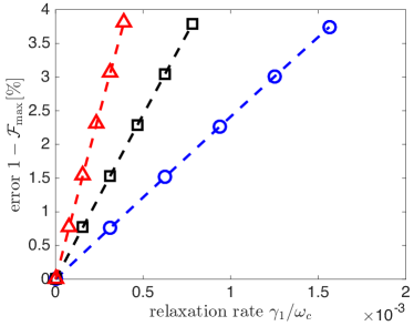
Figure 19: (color online). Relaxation-induced error $\xi_{\gamma}$ for $g/\omega_{c}=1/8$ (blue circles), $g/\omega_{c}=1/\left(8\sqrt{2}\right)$ (black squares) and $g/\omega_{c}=1/16$ (red diamonds). Other numerical parameters: $k_{B}T/\omega_{c}=0.01$, $\kappa=0$, $\Gamma=0$ and $\omega_{q}=0$.

To quantitatively capture the effect of relaxation-induced errors, we have analyzed the master equation

$$\dot{\rho}=-i\left[H,\rho\right]+\gamma_{1}\sum_{i}\mathcal{D}\left[\sigma_{i}^{-}\right]\rho,$$ (160)

where the first term refers to the ideal, coherent dynamics and the second term describes single-spin relaxation with a rate $\gamma_{1}=T_{1}^{-1}$; incoherent excitation processes could be included as well, with additional terms of the same form with the appropriate replacement $\sigma_{i}^{-}\rightarrow\sigma_{i}^{+}$, but are omitted here for clarity. Along the lines of our analysis for dephasing-induced errors, the relaxation-induced error is expected to scale linearly with the relaxation rate as $\xi_{\gamma}\sim\gamma_{1}/g_{\mathrm{eff}}$, that is

$$\xi_{\gamma}\approx\alpha_{\gamma}\frac{\gamma_{1}}{\omega_{c}},$$ (161)

with the pre-factor $\alpha_{\gamma}=c_{\gamma}/\mu^{2}$, where $\mu=g/\omega_{c}$. As shown in Fig.19, based on numerical simulations of Eq.(160), this linear error scaling has been verified numerically, yielding the numerical pre-factor $c_{\gamma}\approx 0.38$, that is $\alpha_{\gamma}\approx 0.38/\mu^{2}$. This numerical pre-factor coincides very well with the value obtained for the dephasing-induced error $\sim\Gamma$ (when properly accounting for the factor of four in our definition $\Gamma=2/T_{2}^{\star}$; compare the corresponding master equation Eq.(7) in the main text); recall $\xi_{\Gamma}\approx\alpha_{\Gamma}\Gamma/\omega_{c}=4\alpha_{\Gamma}\gamma_{\phi}/\omega_{c}$, with $4\alpha_{\Gamma}\approx 0.4/\mu^{2}$ and $\gamma_{\phi}\equiv\Gamma/4$ (to match with our definition of $\gamma_{1}$). Accordingly, in the typical scenario where $T_{2}^{\star}\ll T_{1}$ (as discussed in the previous subsection), indeed relaxation-induced errors (as well as similar incoherent excitation processes) can be safely neglected. In the opposite regime, where pure-dephasing processes are negligible (such that the decoherence timescale reaches its fundamental upper limit $T_{2}\leq 2T_{1}$, i.e. the qubit coherence is limited by spin flips), the total error $\xi_{\mathrm{dec}}$ induced by qubit decoherence is simply given by $\xi_{\mathrm{dec}}\approx\xi_{\gamma}\approx\alpha_{\gamma}\gamma_{1}/\omega_{c}$. Finally, in the worst-case regime where the pure-dephasing rate and the relaxation rate are comparable $\left(\gamma_{\phi}\approx\gamma_{1}\right)$, the total error due to qubit decoherence amounts to $\xi_{\mathrm{dec}}=\xi_{\gamma}+\xi_{\Gamma}\approx 2\alpha_{\gamma}\gamma_{1}/\omega_{c}\approx 2\alpha_{\Gamma}\Gamma/\omega_{c}$, i.e. just a factor of two larger than the decoherence-induced error considered in the main text.

Appendix O Average Gate Fidelity

Figure 20: (color online). Total average gate error $\bar{E}$ (in percent) as a function of both the effective rethermalization rate $\sim\kappa/\omega_{c}\bar{n}_{\mathrm{th}}\sim\bar{n}_{\mathrm{th}}/Q$ and the spin dephasing rate $\sim\Gamma/\omega_{c}$ for $g/\omega_{c}=1/4$ (top) and $g/\omega_{c}=1/8$ (bottom). Other numerical parameters: $k_{B}T/\omega_{c}=2$ and $\omega_{q}=0$.

The average gate fidelity $\bar{F}$ is a useful measure in order to quantify how well the completely-positive, trace-preserving quantum operation $\mathcal{M}$ (in the presence of noise) approximates a given unitary gate $U_{\mathrm{id}}$, which represents the ideal (noise-free) evolution. Formally, it is defined as

$$\bar{F}=\int d\psi\left<\psi\right|U_{\mathrm{id}}^{\dagger}\mathcal{M}\left(\left|\psi\right\rangle\left\langle\psi\right|\right)U_{\mathrm{id}}\left|\psi\right>,$$ (162)

where the integral runs over the uniform (Haar) measure $d\psi$ on state space, with $\int d\psi=1$ nielsen02-sm . As shown in Ref.nielsen02-sm , $\bar{F}$ may be re-expressed as

$$\bar{F}=\frac{dF_{\mathrm{ent}}+1}{d+1},$$ (163)

where $d$ is the dimension of the Hilbert space ($d=4$ for two qubits) and the entanglement fidelity $F_{\mathrm{ent}}$ is the fidelity of the state obtained when $\mathcal{M}$ acts on one half of a maximally entangled state with the state obtained from the action of the ideal evolution; it is given by

$$F_{\mathrm{ent}}=\frac{1}{d^{3}}\sum_{P\in G}\mathrm{tr}\left[P^{\dagger}U_{\mathrm{id}}^{\dagger}\mathcal{M}\left(P\right)U_{\mathrm{id}}\right].$$ (164)

Here, $G$ is a set of $d\times d$ unitary operators, forming a basis for a qudit, i.e., $\mathrm{tr}\left[P_{j}^{\dagger}P_{k}\right]=\delta_{jk}d$, $j,k=1,\dots,d^{2}$. For two qubits we may take the set of Pauli matrices modulo phase, comprising in total 16 operators $G=\left\{\mathds{1},\sigma_{i}^{\alpha},\sigma_{1}^{\alpha}\sigma_{2}^{\beta}\right\}$, with $i=1,2$, $\alpha=x,y,z$. Experimentally, $\bar{F}$ may be determined using standard state tomography nielsen02-sm .

Errors.—The average gate error (infidelity) is defined as $\bar{E}=1-\bar{F}$. As follows directly from Eq.(163), it is related to the entanglement infidelity $E_{\mathrm{ent}}=1-F_{\mathrm{ent}}$ via $\bar{E}=d/\left(d+1\right)\times E_{\mathrm{ent}}$; thus, for two qubits $\bar{E}=\left(4/5\right)E_{\mathrm{ent}}$.

Numerical results.—Numerical results for the average gate error $\bar{E}$ are presented in Fig.20. Here, the map $\mathcal{M}\left(P\right)$ is given implicitly as $\mathcal{M}\left(P\right)=\mathrm{tr}_{a}\left[e^{\mathcal{L}t_{\mathrm{max}}}P\otimes\rho_{\mathrm{th}}\right]$, where the superoperator $\mathcal{L}\bullet=-i\left[H,\bullet\right]+\mathcal{L}_{\mathrm{noise}}\bullet$ is the Liouvillian associated with the master equation given in Eq.(7) in the main text, which includes undesired processes due to rethermalization of the cavity mode and dephasing of the spins. Broadly speaking, our numerical results for the (average) gate error $\bar{E}$ are comparable to the ones obtained for the state infidelity $\xi=1-\mathcal{F}$, as discussed in the main text. First, comparison of our results for $g/\omega_{c}=1/4$ and $g/\omega_{c}=1/8$ shows that rethermalization-induced errors are approximately independent of the spin-resonator coupling $g$; for example, for $\Gamma=0$ and $\kappa/\omega_{c}\bar{n}_{\mathrm{th}}=2.5\times 10^{-3}$ we find $\bar{E}_{\kappa}\approx 0.82\%$ for both $g/\omega_{c}=1/4$ and $g/\omega_{c}=1/8$, respectively. Second, as expected, the dephasing induced error scales as $\bar{E}_{\Gamma}\sim 1/g^{2}\sim 1/\mu^{2}$; for example, as shown in Fig.20, for $\kappa=0$ and $\Gamma/\omega_{c}=1.5\times 10^{-3}$, we find $\bar{E}_{\Gamma}\approx 0.376\%$ and $\bar{E}_{\Gamma}\approx 1.49\%\approx 4\times 0.376\%$ for $g/\omega_{c}=1/4$ and $g/\omega_{c}=1/8$, respectively.

References

- (1) R. Hanson and D. D. Awschalom, Nature 453, 1043 (2008).
- (2) M. A. Nielsen and I. L. Chuang, Quantum Computation and Quantum Information (Cambridge University Press, 2010).
- (3) L. R. Schreiber and H. Bluhm, Nature Nanotech. 9, 966 (2014).
- (4) E. Knill, Nature 434, 39 (2005).
- (5) N. H. Nickerson, Y. Li, and S. C. Benjamin, Nat. Commun. 4, 1756 (2013).
- (6) J. Majer et al., Nature 449, 443 (2007).
- (7) M. A. Sillanpää, J. I. Park, and R. W. Simmonds, Nature 449, 438 (2007).
- (8) F. Schmidt-Kaler et al., Nature 422, 408 (2003).
- (9) A. Sorensen and K. Molmer, Phys. Rev. Lett. 82, 1971 (1999).
- (10) A. Sorensen and K. Molmer, Phys. Rev. A 62, 022311 (2000).
- (11) K. Molmer and A. Sorensen, Phys. Rev. Lett. 82, 1835 (1999).
- (12) G. J. Milburn, arXiv:quant-ph/9908037 (unpublished).
- (13) G. J. Milburn, S. Schneider, and D. F. V. James, Fortschr. Phys. 48, 801 (2000).
- (14) J. F. Poyatos, J. I. Cirac, and P. Zoller, Phys. Rev. Lett. 81, 1322 (1998).
- (15) J. I. Cirac and P. Zoller, Nature 404, 579 (2000).
- (16) J. J. Garcia-Ripoll, P. Zoller, and J. I. Cirac, Phys. Rev. Lett. 91, 157901 (2003).
- (17) J. J. Garcia-Ripoll, P. Zoller, and J. I. Cirac, Phys. Rev. A 71, 062309 (2005).
- (18) D. Porras and J. I. Cirac, Phys. Rev. Lett. 92, 207901 (2004).
- (19) D. Leibfried et al., Nature 422, 412 (2003).
- (20) G. Kirchmair, J. Benhelm, F. Zähringer, R. Gerritsma, C. F. Roos and R. Blatt, New J. Phys. 11, 023002 (2009).
- (21) A. J. Kerman, New Journal of Physics 15, 123011 (2013).
- (22) B. Royer, A. L. Grimsmo, N. Didier, and A. Blais, arXiv:1603.04424 (unpublished).
- (23) D. J. Reilly, NPJ Quantum Information 1, 15011 (2015).
- (24) P. Treutlein, C. Genes, K. Hammerer, M. Poggio, and P. Rabl, "Hybrid Mechanical Systems", in: "Cavity Optomechanics", ed. by M. Aspelmeyer, T. J. Kippenberg, and F. Marquardt (Springer, Berlin 2014) pp. 327-351.
- (25) A. Blais, R.-S. Huang, A. Wallraff, S. M. Girvin, and R. J. Schoelkopf, Phys. Rev. A 69, 062320 (2004).
- (26) L. Childress, A. S. Sorensen, and M. D. Lukin, Phys. Rev. A 69, 042302 (2004).
- (27) J. M. Taylor and M. D. Lukin, arXiv:cond-mat/0605144 (unpublished).
- (28) P.-Q. Jin, M. Marthaler, A. Shnirman, and G. Schon, Phys. Rev. Lett. 108, 190506 (2012).
- (29) X. Hu, Y.-x. Liu, and F. Nori, Phys. Rev. B 86, 035314 (2012).
- (30) M. Trif, V. N. Golovach, and D. Loss, Phys. Rev. B 77, 045434 (2008).
- (31) M. J. Gullans, Y.-Y. Liu, J. Stehlik, J. R. Petta, and J. M. Taylor, Phys. Rev. Lett. 114, 196802 (2015).
- (32) P.-Q. Jin, M. Marthaler, J. H. Cole, A. Shnirman, and G. Schon, Phys. Rev. B 84, 035322 (2011).
- (33) M. Kulkarni, O. Cotlet, and H. E. Tureci, Phys. Rev. B 90, 125402 (2014).
- (34) V. Srinivasa, J. M. Taylor, and C. Tahan, Phys. Rev. B 94, 205421 (2016).
- (35) T. Frey, P. J. Leek, M. Beck, A. Blais, T. Ihn, K. Ensslin, and A. Wallraff, Phys. Rev. Lett. 108, 046807 (2012).
- (36) K. D. Petersson, L. W. McFaul, M. D. Schroer, M. Jung, J. M. Taylor, A. A. Houck, and J. R. Petta, Nature 490, 380 (2012).
- (37) Y.-Y. Liu, K. D. Petersson, J. Stehlik, J. M. Taylor, and J. R. Petta, Phys. Rev. Lett. 113, 036801 (2014).
- (38) H. Toida, T. Nakajima, and S. Komiyama, Phys. Rev. Lett. 110, 066802 (2013). Also see: A. Wallraff, A. Stockklauser, T. Ihn, J. R. Petta, and A. Blais, Phys. Rev. Lett. 111, 249701 (2013).
- (39) M. R. Delbecq, V. Schmitt, F. D. Parmentier, N. Roch, J. J. Viennot, G. Feve, B. Huard, C. Mora, A. Cottet, and T. Kontos, Phys. Rev. Lett. 107, 256804 (2011).
- (40) J. J. Viennot, M. R. Delbecq, M. C. Dartiailh, A. Cottet, and T. Kontos, Phys. Rev. B 89, 165404 (2014).
- (41) J. J. Viennot, M. C. Dartiailh, A. Cottet, and T. Kontos, Science 349, 408 (2015).
- (42) L. J. Zou, D. Marcos, S. Diehl, S. Putz, J. Schmiedmayer, J. Majer, and P. Rabl, Phys. Rev. Lett. 113, 023603 (2014).
- (43) F. Beaudoin, D. Lachance-Quirion, W. A. Coish, M. Pioro-Ladriere, Nanotechnology 27, 464003 (2016).
- (44) X. Mi, J. V. Cady, D. M. Zajac, P. W. Deelman, and J. R. Petta, Science 355, 126 (2017).
- (45) A. Stockklauser, P. Scarlino, J. V. Koski, S. Gasparinetti, C. K. Andersen, C. Reichl, W. Wegscheider, T. Ihn, K. Ensslin, and A. Wallraff, Phys. Rev. X 7, 011030 (2017).
- (46) M. J. A. Schuetz, E. M. Kessler, G. Giedke, L. M. K. Vandersypen, M. D. Lukin, and J. I. Cirac, Phys. Rev. X 5, 031031 (2015).
- (47) J. C. Chen, Y. Sato, R. Kosaka, M. Hashisaka, K. Muraki, and T. Fujisawa, Sci. Rep. 5, 15176 (2015).
- (48) D. A. Golter, T. Oo, M. Amezcua, K. A. Stewart, and H. Wang, Phys. Rev. Lett. 116, 143602 (2016).
- (49) P. Rabl, P. Cappellaro, M. V. Gurudev Dutt, L. Jiang, J. R. Maze, and M. D. Lukin, Phys. Rev. B 79, 041302(R) (2009).
- (50) P. Rabl, S. J. Kolkowitz, F. H. L. Koppens, J. G. E. Harris, P. Zoller, and M. D. Lukin, Nat. Phys. 6, 602 (2010).
- (51) K. V. Kepesidis, S. D. Bennett, S. Portolan, M. D. Lukin, and P. Rabl, Phys. Rev. B 88, 064105 (2013).
- (52) S. D. Bennett, N. Y. Yao, J. Otterbach, P. Zoller, P. Rabl, and M. D. Lukin, Phys. Rev. Lett. 110, 156402 (2013).
- (53) A. Palyi, P. R. Struck, M. Rudner, K. Flensberg, and G. Burkard, Phys. Rev. Lett. 108, 206811 (2012).
- (54) C. Cohen-Tannoudji, J. Dupont-Roc, and G. Grynberg, Atom-Photon Interactions: Basic Processes and Applications (Wiley, New York, 1992).
- (55) R. J. Schoelkopf and S. M. Girvin, Nature 451, 664 (2008).
- (56) N. Samkharadze, A. Bruno, P. Scarlino, G. Zheng, D. P. DiVincenzo, L. DiCarlo, and L. M. K. Vandersypen, Phys. Rev. Applied 5, 044004 (2016).
- (57) R. Barends, J. J. A. Baselmans, S. J. C. Yates, J. R. Gao, J. N. Hovenier, and T. M. Klapwijk, Phys. Rev. Lett. 100, 257002 (2008).
- (58) M. Veldhorst et al., Nature Nano. 9, 981 (2014).
- (59) Chow et al., Phys. Rev. Lett. 109, 060501 (2012).
- (60) R. Hanson, L. P. Kouwenhoven, J. R. Petta, S. Tarucha, and L. M. K. Vandersypen, Rev. Mod. Phys. 79, 1217 (2007).
- (61) J. Levy, Phys. Rev. Lett. 89, 147902 (2002).
- (62) K. E. Cahill and R. J. Glauber, Phys. Rev. 177, 1857 (1969).
- (63) M. V. Gustafsson, P. V. Santos, G. Johansson, and P. Delsing, Nat. Phys. 8, 338 (2012).
- (64) R. Manenti, M. J. Peterer, A. Nersisyan, E. B. Magnusson, A. Patterson, and P. J. Leek, Phys. Rev. B 93, 041411(R) (2016).
- (65) F. K. Malinowski et al., Nat. Nanotechnol. 12, 16 (2017).
- (66) P. Zoller, Quantum Optics: Continous Measurement, Stochastic Schrödinger Equations, Master Equations etc., lecture notes, available online (http://www.coqus.at/fileadmin/quantum/coqus /documents/Klemens_Hammerer/QO_Zoller_Lecture2-Continous_Measurement.pdf).
- (67) P. Rabl, Advanced Quantum Optics, lecture notes TU Vienna (2014).
- (68) P.-O. Guimond, H. Pichler, A. Rauschenbeutel, and P. Zoller, Phys. Rev. A 94, 033829 (2016).
- (69) C. W. Gardiner and P. Zoller, Quantum Noise (Springer, Berlin, 2000).
- (70) Y. Yamamoto and A. Imamoglu, Mesoscopic Quantum Optics (Wiley, New York, 1999).
- (71) H. J. Carmichael, Statistical Methods in Quantum Optics 1 (Springer, Berlin, 2002).
- (72) I. de Vega and D. Alonso, Rev. Mod. Phys. 89, 15001 (2017).
- (73) J. Paavola, Role of the environmental spectrum in the decoherence and dissipation of a quantum Brownian particle, Master’s thesis, University of Turku, 2008.
- (74) F. Beaudoin, J. M. Gambetta, and A. Blais, Phys. Rev. A 84, 043832 (2011).
- (75) M. Scala, B. Militello, A. Messina, S. Maniscalco, J. Piilo, and K. A. Suominen, J. Phys. A: Math. Theor. 40, 14527 (2007).
- (76) A. Blais, J. Gambetta, A. Wallraff, D. I. Schuster, S. M. Girvin, M. H. Devoret, and R. J. Schoelkopf, Phys. Rev. A 75, 032329 (2007).
- (77) H. Wang and G. Burkard, Phys. Rev. B 92, 195432 (2015).
- (78) E. Bocquillon et al., Science 339, 1054 (2013).
- (79) V. Kornich, C. Kloeffel, and D. Loss, Phys. Rev. B 89, 085410 (2014).
- (80) C. Kloeffel and D. Loss, Annu. Rev. Condens. Matter Phys. 4, 51 (2013).
- (81) M. Kroutvar, Y. Ducommun, D. Heiss, M. Bichler, D. Schuh, G. Abstreiter, and J. J. Finley, Nature 432, 81 (2004).
- (82) S. Amasha, K. MacLean, I. P. Radu, D. M. Zumbuhl, M. A. Kastner, M. P. Hanson, and A. C. Gossard, Phys. Rev. Lett. 100, 046803 (2008).
- (83) L. M. Woods, T. L. Reinecke, and Y. Lyanda-Geller, Phys. Rev. B 66, 161318 (2002).
- (84) A. V. Khaetskii and Y. V. Nazarov, Phys. Rev. B 64, 125316 (2001).
- (85) T. Meunier et al., Phys. Rev. Lett. 98, 126601 (2007).
- (86) C. B. Simmons et al., Phys. Rev. Lett. 106, 156804 (2011).
- (87) J. R. Prance et al., Phys. Rev. Lett. 108, 046808 (2012).
- (88) H. Christ, J. I. Cirac, and G. Giedke, Phys. Rev. B 78, 125314 (2008).
- (89) R. Amsüss et al., Phys. Rev. Lett. 107, 060502 (2011).
- (90) J. Harrison, M. Sellars, and N. Manson, Diam. Relat. Mater. 15, 586 (2006).
- (91) A. Jarmola, V. M. Acosta, K. Jensen, S. Chemerisov, and D. Budker, Phys. Rev. Lett. 108, 197601 (2012).
- (92) A. Barfuss, J. Teissier, E .Neu, A. Nunnenkamp, and P. Maletinsky, Nature Phys. 11, 820 (2015).
- (93) J. Teissier, A. Barfuss, P. Appel, E. Neu, and P. Maletinsky, Phys. Rev. Lett. 113, 020503 (2014).
- (94) P. C. Maurer et al., Science 336, 1283 (2012).
- (95) M. A. Nielsen, Phys. Lett. A 303, 249 (2002).