Fractional Order Optimal Control Model For Malaria Infection

Abstract

We propose and study an optimal control model for malaria infection described by system of fractional differential equations. The model is formulated in terms of the left and right Caputo fractional derivatives. We determine the necessary conditions for the optimality of the controlled dynamical system. The forward-backward sweep method with generalized euler scheme is applied to numerically compute the solutions of the optimality system.

Keywords: Malaria Infection, Optimal Control Model, Fractional Differential Equations.

1 Introduction

Mathematical modeling of malaria infection using differential equations with integer order and non-integer derivatives have been considered by many authors (see, e.g, Pinto and Machado, 2013, Okyere et al., 2016, Ngonghala et al., 2012, Ross, 1911, Abdullahi et al., 2013, Keegan and Dushoff, 2013, Chitnis et al., 2006). A comprehensive survey on malaria infection modeling has been captured in the work by Mandal et al. (2011). Infectious diseases prevention and control strategies are very important factors and if properly addressed can go a long way in reducing disease infections in a population. Optimal control theory is one of the useful and efficient modeling tools that can help in the modeling framework to better understand the dynamics of the disease and suggest possible prevention and control measures. In recent times, malaria modeling formulation based on optimal control theory with time dependent controls has attracted much attention (see, e.g, Okosun et al., 2013, Otieno et al., 2016, Athithan and Ghosh, 2015, Augsto et al., 2012, Mwanga et al., 2014, Silva and Torres, 2013, Okosun and Makinde, 2014, 2011).

The paper by Lashari and Zaman (2012) proposed and numerically analyzed an optimal control model to investigate the effectiveness of time dependent controls on vector-borne diseases. From the numerical results, they (Lashari and Zaman, 2012) observed that, optimal control strategies are effective in reducing the infected populations. Lashari et al. (2012) proposed a time dependent multiple controls to study malaria infection. The authors in (Blayneh et al., 2009) formulated a time dependent treatment and prevention optimal control model to study vector-borne diseases. Okosun and Makinde (2013) presented a controlled dynamical malaria model based on non-linear incidence. Kim et al. (2013) developed a dynamic control problem to study malaria transmission using two time dependent control functions.

The Ebola infection that claimed many lives in Africa has also been considered with optimal control theory (see, e.g, Rachah and Torres, 2016, Bonyah et al., 2016, Grigorieva and Khailov, 2015). Compartmental models for infectious diseases such as TB, HIV and Cholera with time dependent controls have been studied (see, e.g, Moualeu et al., 2015, Magombedze et al., 2011, Bakhtiar, 2016, Choi et al., 2015).

Fractional order derivative has an important property called memory effect and because of that, the theory and application of fractional calculus have widely been used to model dynamical processes in the field of science, engineering and many others (see, e.g, Petras, 2011, Podlubny, 1999). Agrawal (2004) developed general optimal control problems that are driven by Riemann-Liouville fractional derivatives. In another research by the same author (Agrawal, 2008a), he formulated similar optimal control problems with Caputo derivatives and developed a stable numerical scheme for the mathematical model.

Several researchers have developed and analyzed optimal control problems whereby the controlled dynamic problems are characterised by Riemann-Liouville derivatives (see, e.g, Frederico and Torres, 2008, Tricaud and Chen, 2010, Agrawal et al., 2010, Agrawal and Baleanu, 2007). An enzyme kinetic optimal control problem was proposed and numerically studied by Basir et al. (2015). The authors in (Ding et al., 2012) studeid HIV-Immune System model using fractional optimal control. They deduced the necessary conditions for the optimality system for a general control problem with Caputo derivatives using the concept of calculus of variation and fractional integration by parts formula. Necessary optimality conditions have been derived for an optimal control problem whereby the state model had both first order derivative and non-integer derivative (Pooseh et al., 2014).

It has been demonstrated in literature that optimal control problems are appropriate for biological systems and other processes that follow non-linear behavior. Therefore modeling infectious diseases using fractional derivatives together with optimal control theory is a huge advantage. Okyere et al. (2016) extended the malaria infection model by Tumwiine et al. (2007a, b) to include fractional derivatives. They (Okyere et al., 2016) investigated asymptotic analysis of the model equilibria and solved the dynamical problem with the numerical scheme developed by Diethelm et al. (2004, 2002). In this work, we propose a fractional optimal control model for malaria infection and numerically simulate the solutions of the constructed control problem. We extend the malaria epidemic model studied by the authors in (Tumwiine et al., 2007a, b) to become an optimal control problem of which the state and costate equations are characterised by differential equations of fractional orders. Our model formulation is different from previous works on malaria disease modeling since we have incorporated fractional order derivatives into the controlled dynamical system.

The paper is organized as follows. Section 2 deals with brief review on the mathematical formulation of fractional optimal control problem. We formulate the controlled malaria model and deduce the necessary conditions for the optimality of the model problem in section 3. Section 4 deals with numerical solutions and discussions of simulations results. We then conclude the paper in section 5.

2 Optimal Control Problem With Fractional Derivatives

This section deals with brief review on the mathematical formulation of fractional optimal control model. We will then apply the modeling concept to formulate our new malaria model in section 3. There are many types of fractional derivatives but the most used ones in mathematical modeling and engineering applications are Riemann-Liouville derivative and Caputo derivative (see, e.g, Petras, 2011, Podlubny, 1999). For this work, we develop the optimization model with Caputo fractional derivatives..

Definition 1

(Podlubny, 1999, Pooseh et al., 2014) The left Caputo fractional derivative is defined as

$${}_{a}^{c}D^{\alpha}_{t}w(t)=\frac{1}{\Gamma(p-\alpha)}\int_{a}^{t}\!\frac{w^{(p)}(x)}{(t-x)^{\alpha+1-p}}\,\mathrm{d}x.$$

for $p-1<\alpha<p.$

Definition 2

(Podlubny, 1999, Pooseh et al., 2014) The right Caputo fractional derivative is defined as

$${}_{t}^{c}D^{\alpha}_{b}w(t)=\frac{(-1)^{p}}{\Gamma(p-\alpha)}\int_{t}^{b}\!\frac{w^{(p)}(x)}{(x-t)^{\alpha+1-p}}\,\mathrm{d}x.$$

for $p-1<\alpha<p,$

where $\alpha$ is the order of the Caputo derivatives.

In the works by Agrawal (2008a, b), he formulated an optimal control problem with Caputo fractional derivatives as follows. Find an optimal control $u$ that minimise the objective functional or performance index:

$$J(u)=\int_{0}^{1}\!W(x,u,t)\,\mathrm{d}t.$$ (1)

Subject to the fractional dynamic constraint

$$_{0}^{c}D^{\alpha}_{t}x(t)=M(x,u,t)$$ (2)

with initial condition

$$x(0)=x_{o},$$ (3)

where $W(x,u,t)$ and $M(x,u,t)$ are two arbitrary functions and $x(t)$ is the state variable (Agrawal, 2004, 2008a). By using the method of lagrange multipliers, calculus of variation and the integration by parts formula for fractional order derivatives and also following a similar derivation by the same author in (Agrawal, 2004), he obtained the necessary conditions or equations (4-6) for the fractional order controlled problem as follows:

$$_{0}^{c}D^{\alpha}_{t}x(t) =M(x,u,t)$$ (4)

$$_{t}^{c}D^{\alpha}_{1}x(t) =\frac{\partial W}{\partial x}+\lambda\frac{\partial M}{\partial x}$$ (5)

$$\frac{\partial W}{\partial u}+\lambda\frac{\partial M}{\partial u} =0$$ (6)

with

$$\begin{cases}x(0)=x_{o}&\\ \\ \lambda(1)=0,\end{cases}$$ (7)

where $\lambda$ is the co-state variable called lagrange multiplier.

3 Controlled Malaria Model With Fractional Derivatives

In this section, we will use the obtained results in the optimal control problem formulation briefly reviewed in section 2 to deduce our necessary conditions or equations for the optimality of the optimal control malaria model. Our model formulation seeks to find an optimal control that would minimise the infected human populations and the cost of implementing the optimal control and prevention strategies. In this work, we consider three time dependent controls namely treated bednets, treatment and insecticide spray.

The main aim in our present formulation is to find optimal control $U$ that minimise the objective functional:

$$J(U)=\int_{0}^{b}\!W(X,U,t)\,\mathrm{d}t.$$ (8)

Subject to the fractional dynamic constraints

$$_{0}^{c}D^{\alpha}_{t}X(t)=M(X,U,t)$$ (9)

with initial condition

$$X(0)=X_{o}$$ (10)

where

$$X(t) =(S_{H},I_{H},R_{H},S_{V},I_{V})^{T}$$

$$X(0) =(S_{H}(0),I_{H}(0),R_{H}(0),S_{V}(0),I_{V}(0))^{T}$$

$$U(t) =(u_{1},u_{1},u_{3})^{T}$$

$$W(X,U,t) =AI_{H}+\frac{d_{1}u^{2}_{1}}{2}+\frac{d_{2}u^{2}_{2}}{2}+\frac{d_{3}u^{2}_{3}}{2}$$

$$M(X,U,t)=\left[\begin{array}[]{c}\lambda^{\alpha}_{h}N_{H}-\frac{(1-u_{1})a^{\alpha}bS_{H}I_{V}}{N_{H}}+\nu^{\alpha}I_{H}+\gamma^{\alpha}R_{H}-\mu^{\alpha}_{h}S_{H}\\ \\ \frac{(1-u_{1})a^{\alpha}bS_{H}I_{V}}{N_{H}}-\nu^{\alpha}I_{H}-(r^{\alpha}+\rho^{\alpha}u_{2})I_{H}-\delta^{\alpha}I_{H}-\mu^{\alpha}_{h}I_{H}\\ \\ (r^{\alpha}+\rho^{\alpha}u_{2})I_{H}-(\gamma^{\alpha}+\mu^{\alpha}_{h})R_{H}\\ \\ (1-u_{3})\lambda^{\alpha}_{v}N_{V}-\frac{(1-u_{1})a^{\alpha}cS_{V}I_{H}}{N_{H}}-\mu^{\alpha}_{v}S_{V}-\eta^{\alpha}u_{3}S_{V}\\ \\ \frac{(1-u_{1})a^{\alpha}cS_{V}I_{H}}{N_{H}}-\mu^{\alpha}_{v}I_{V}-\eta^{\alpha}u_{3}I_{V}\end{array}\right]$$ (20)

The variable $X(t)$ is the state vector and $U$ is the control vector. As in Agrawal (2004, 2008b), when $\alpha=1$, the formulated malaria controlled dynamical model becomes classical optimal control problem for the uncontrolled malaria model proposed and analyzed by Tumwiine et al. (2007a, b). Also note that, when $\alpha=1$, with control functions $u_{1}=u_{2}=u_{3}=0$, then the dynamic constraint equation (9) with the initial condition (10) becomes the malaria infection model developed by the authors in (Tumwiine et al., 2007a, b)

The meaning of the model variables and time dependent optimal control functions are defined in table 1. The definitions for the model parameters can be found in table 2

Table 1: Description of model variables and control functions.

Model variables and control functions	Description
$S_{H}$	Susceptible human class
$I_{H}$	Infected human class
$R_{H}$	partially immune human class
$S_{V}$	Susceptible mosquito class
$I_{V}$	Infected mosquito class
$N_{H}$	Total human population
$N_{V}$	Total mosquito population
$u_{1}$	The control on the use of treated bednets
$u_{2}$	The control on treatment of infected individuals
$u_{3}$	The control on the use of insecticide spray

Table 2: Description of model parameters.

Model Parameters	Description
$\lambda_{h}$	natural birth rate of humans
$\lambda_{v}$	natural birth rate of mosquitoes
$\mu_{h}$	natural death rate of humans
$\mu_{v}$	natural death rate of mosquitoes
$a$	average daily biting rate on human by a single mosquito
$b$	proportion of bites on human that produce an infection
$\delta$	death rate due to the disease
$c$	probability that a mosquito becomes infectious
$\nu$	recovery rate of human hosts from the disease
$\gamma$	rate of loss of immunity in human hosts
$r$	rate at which human hosts acquire immunity
$\rho$	rate constant due to treatment
$\eta$	rate constant due to insecticide spray
$A,\ d_{1},\ d_{2},\ d_{3}$	weight constants

It is important to mention that, rigorous proofs on the derivation of necessary conditions for the optimality of various fractional dynamical systems can be found in literature (see, e.g, Pooseh et al., 2014, Ding et al., 2012, Agrawal, 2004). Therefore in this paper, using the ideas by the authors in (see, e.g, Agrawal, 2008a, b, Pooseh et al., 2014, Ding et al., 2012, Agrawal, 2004), we state the necessary conditions (21-23) for our optimization problem as follows:

$$_{0}^{c}D^{\alpha}_{t}X(t) =M(X,U,t)$$ (21)

$$_{t}^{c}D^{\alpha}_{b}\lambda(t) =\frac{\partial W}{\partial X}+\lambda^{T}\frac{\partial M}{\partial X}$$ (22)

$$\frac{\partial W}{\partial U}+\lambda^{T}\frac{\partial M}{\partial U} =0$$ (23)

and

$$\begin{cases}X(0)=X_{o}&\\ \lambda(b)=0\end{cases}$$ (24)

where $\lambda(t)=(\lambda_{1},\lambda_{2},\lambda_{3},\lambda_{4},\lambda_{5})^{T}$ is the co-state vector.

Now using the compact form of the necessary conditions stated above, we obtain the optimality system for the fractional optimal control malaria model in an expanded form as follows:

$$\begin{array}[]{lllll}{}_{0}^{c}D^{\alpha}_{t}S_{H}&=&\displaystyle{\lambda^{\alpha}_{h}N_{H}-\frac{(1-u_{1})a^{\alpha}bS_{H}I_{V}}{N_{H}}+\nu^{\alpha}I_{H}+\gamma^{\alpha}R_{H}-\mu^{\alpha}_{h}S_{H}},\\[15.0pt] {}_{0}^{c}D^{\alpha}_{t}I_{H}&=&\displaystyle{\frac{(1-u_{1})a^{\alpha}bS_{H}I_{V}}{N_{H}}-\nu^{\alpha}I_{H}-(r^{\alpha}+\rho^{\alpha}u_{2})I_{H}-\delta^{\alpha}I_{H}-\mu^{\alpha}_{h}I_{H}},\\[15.0pt] {}_{0}^{c}D^{\alpha}_{t}R_{H}&=&\displaystyle{(r^{\alpha}+\rho^{\alpha}u_{2})I_{H}-(\gamma^{\alpha}+\mu^{\alpha}_{h})R_{H}},\\[15.0pt] {}_{0}^{c}D^{\alpha}_{t}S_{V}&=&\displaystyle{(1-u_{3})\lambda^{\alpha}_{v}N_{V}-\frac{(1-u_{1})a^{\alpha}cS_{V}I_{H}}{N_{H}}-\mu^{\alpha}_{v}S_{V}-\eta^{\alpha}u_{3}S_{V}},\\[15.0pt] {}_{0}^{c}D^{\alpha}_{t}I_{V}&=&\displaystyle{\frac{(1-u_{1})a^{\alpha}cS_{V}I_{H}}{N_{H}}-\mu^{\alpha}_{v}I_{V}-\eta^{\alpha}u_{3}I_{V}},\end{array}$$ (25)

$$\begin{cases}{}_{t}^{c}D^{\alpha}_{b}\lambda_{1}=&\lambda_{1}\left[\lambda^{\alpha}_{h}-\dfrac{(1-u_{1})(I_{H}+R_{H})a^{\alpha}bI_{V}}{N^{2}_{H}}-\mu^{\alpha}_{h}\right]+\lambda_{2}\left[\dfrac{(1-u_{1})(I_{H}+R_{H})a^{\alpha}bI_{V}}{N^{2}_{H}}\right]\\ \\ &-(\lambda_{5}-\lambda_{4})\left[\dfrac{(1-u_{1}))a^{\alpha}cS_{H}I_{H}}{N^{2}_{H}}\right]\\ \\ {}_{t}^{c}D^{\alpha}_{b}\lambda_{2}=&A+\lambda_{1}\left[\lambda^{\alpha}_{h}+\dfrac{(1-u_{1})a^{\alpha}bS_{H}I_{V}}{N^{2}_{H}}+\nu^{\alpha}\right]-(\lambda_{4}-\lambda_{5})\left[\dfrac{(1-u_{1})(S_{H}+R_{H})a^{\alpha}cS_{V}}{N^{2}_{H}}\right]\\ \\ &-\lambda_{2}\left[\dfrac{(1-u_{1})a^{\alpha}bS_{H}I_{V}}{N^{2}_{H}}+\nu^{\alpha}+(r^{\alpha}+\rho^{\alpha}u_{2})+\delta^{\alpha}+\mu^{\alpha}_{h}\right]+\lambda_{3}\left[r^{\alpha}+\rho^{\alpha}u_{2}\right]\\ \\ {}_{t}^{c}D^{\alpha}_{b}\lambda_{3}=&\lambda_{1}\left[\lambda^{\alpha}_{h}+\dfrac{(1-u_{1})a^{\alpha}bS_{H}I_{V}}{N^{2}_{H}}+\gamma^{\alpha}_{h}\right]-\lambda_{2}\left[\dfrac{(1-u_{1})a^{\alpha}bS_{H}I_{V}}{N^{2}_{H}}\right]-\lambda_{3}(\gamma^{\alpha}+\mu^{\alpha}_{h})\\ \\ &-(\lambda_{5}-\lambda_{4})\left[\dfrac{(1-u_{1})a^{\alpha}cS_{V}I_{H}}{N^{2}_{H}}\right]\\ \\ {}_{t}^{c}D^{\alpha}_{b}\lambda_{4}=&\lambda_{4}\left[(1-u_{3})\lambda^{\alpha}_{v}+\dfrac{(1-u_{1})a^{\alpha}cI_{H}}{N_{H}}-\mu^{\alpha}_{v}-\eta^{\alpha}u_{3}\right]+\lambda_{5}\left[\dfrac{(1-u_{1})a^{\alpha}cI_{H}}{N_{H}}\right]\\ \\ {}_{t}^{c}D^{\alpha}_{b}\lambda_{5}=&(\lambda_{2}-\lambda_{1})\left[\dfrac{(1-u_{1})a^{\alpha}bS_{H}}{N_{H}}\right]+\lambda_{4}\left[(1-u_{3})\lambda^{\alpha}_{v}\right]-\lambda_{5}\left[\mu^{\alpha}_{v}+\eta^{\alpha}u_{3}\right]\end{cases}$$ (26)

$$\begin{cases}u_{1}=\dfrac{(\lambda_{2}-\lambda_{1})\frac{a^{\alpha}bS_{H}I_{V}}{N_{H}}+(\lambda_{5}-\lambda_{4})\frac{a^{\alpha}cS_{V}I_{H}}{N_{H}}}{B_{1}}&\\ \\ u_{2}=\frac{(\lambda_{2}-\lambda_{3})r^{\alpha}_{o}I_{H}}{B_{2}}&\\ \\ u_{3}=\frac{\lambda_{4}(\lambda^{\alpha}_{v}N_{V}+\eta^{\alpha}S_{V})+\lambda_{5}\eta^{\alpha}I_{V}}{B_{3}}\end{cases}$$ (27)

$$\begin{cases}S_{H}(0)=S_{H_{O}},I_{H}(0)=I_{H_{O}},R_{H}(0)=R_{H_{O}},S_{V}(0)=S_{V_{O}},I_{V}(0)=I_{V_{O}}&\\ \\ \lambda_{1}(b)=0,\lambda_{2}(b)=0,\lambda_{3}(b)=0,\lambda_{4}(b)=0,\lambda_{5}(b)=0,\end{cases}$$ (28)

4 Numerical Simulations and Discussion

The book by Lenhart and Workman (2007) described the numerical solutions of optimal control models for biological systems. In their work, they constructed the forward-backward sweep algorithm with Runge-Kutta method to solve the optimality system of biological models. In this work, the forward-backward algorithm with the generalized euler method is applied to numerically compute the solutions of the optimality system. The generalized euler method is one of the numerical schemes for fractional order models and has recently been applied together with the forward-backward algorithm in a TB model (Sweilam and Al-Mekhlafi, 2016).

The following initial conditions and model parameters values are used for the numerical simulations: $S_{H}(0)=800,\ I_{H}(0)=200,\ R_{H}(0)=20,\ S_{V}(0)=1000,\ I_{V}(0)=500$, $A=100,\ d_{1}=70,\ d_{2}=130,\ d_{3}=40,\ a=0.29,\ b=0.75,\ c=0.75,$ $r=0.05\,\gamma=0.000017,\ \rho=0.7,\ \delta=0.02,\ \nu=0.0022,\ \lambda_{h}=0.0015875,\ \lambda_{v}=0.071,\ \mu_{h}=0.00004,\ \mu_{v}=0.1429,\ \eta=0.25$ and $\alpha=1,\ 0.99,\ 0.95,\ 0.90.$

We considered the following optimal control strategies for our numerical illustrations: Treated bednets control only ($u_{1}\neq 0,\ u_{2}=0,\ u_{3}=0$), treatment control only ($u_{1}=0,\ u_{2}\neq 0,\ u_{3}=0$), insecticide spray control only ($u_{1}=0,\ u_{2}=0,\ u_{3}\neq 0$), treated bednets and treatment controls ($u_{1}\neq 0,\ u_{2}\neq 0,\ u_{3}=0$), treated bednets and insecticide spray controls ($u_{1}\neq 0,\ u_{2}=0,\ u_{3}\neq 0$), treatment and insecticide spray controls ($u_{1}=0,\ u_{2}\neq 0,\ u_{3}\neq 0$), and all the three controls ($u_{1}\neq 0,\ u_{2}\neq 0,\ u_{3}\neq 0$).

From the plots generated, it is clear that reduction of infected human and mosquito populations occurs when $\alpha=1$ (integer order) with time dependent controls but that of non-integer orders ($\alpha=0.99,0.95,0.90$) with time dependent controls are much more significant.

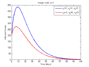
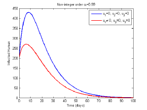
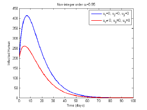
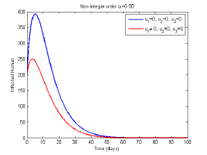
Figure 1: Numerical solutions of infected human host with treated bednets control for $\alpha=1,0.99,0.95,0.90$

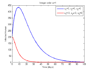
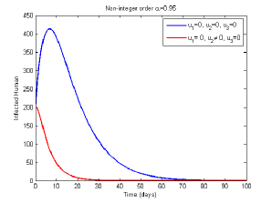
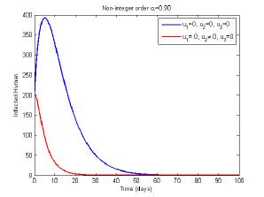
Figure 2: Numerical solutions of infected human host with treatment control for $\alpha=1,0.99,0.95,0.90$

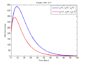
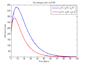
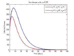
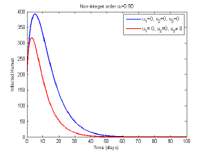
Figure 3: Numerical solutions of infected human host with insecticide spray control for $\alpha=1,0.99,0.95,0.90$

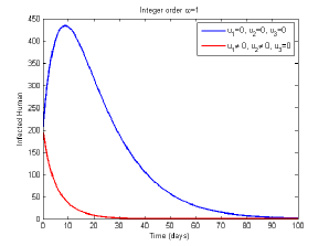
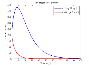
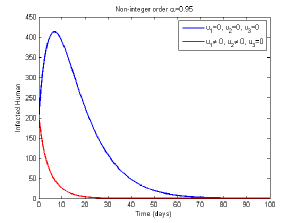
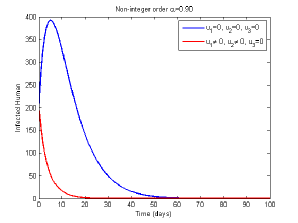
Figure 4: Numerical solutions of infected human host with treated bednets and treatment controls for $\alpha=1,0.99,0.95,0.90$

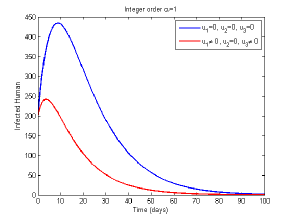
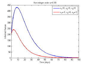
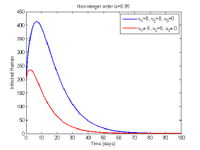
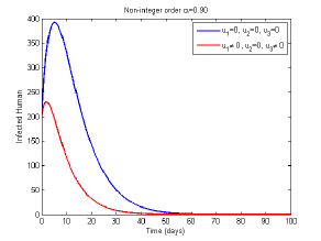
Figure 5: Numerical solutions of infected human host with treated bednets and insecticide spray controls for $\alpha=1,0.99,0.95,0.90$

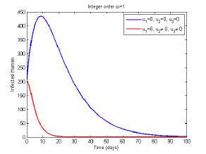
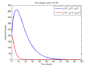
Figure 6: Numerical solutions of infected human host with treatment and insecticide spray controls for $\alpha=1,0.99,0.95,0.90$

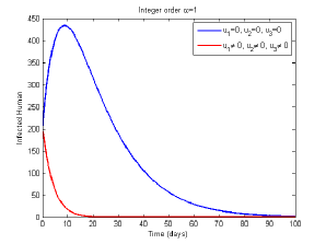
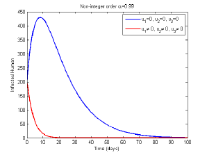
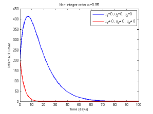
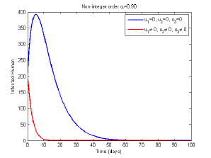
Figure 7: Numerical solutions of infected human host with all the three time dependent optimal controls (treated bednets, treatment and insecticide spray) for $\alpha=1,0.99,0.95,0.90$

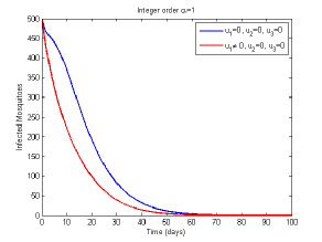
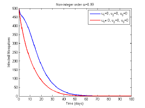
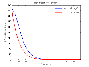
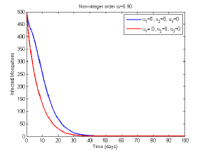
Figure 8: Numerical solutions of infected mosquitoes with treated bednets control for $\alpha=1,0.99,0.95,0.90$

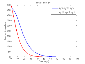
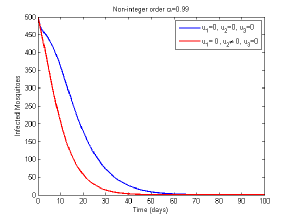
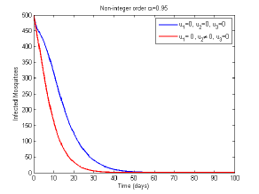
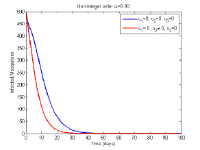
Figure 9: Numerical solutions of infected mosquitoes with treatment control for $\alpha=1,0.99,0.95,0.90$

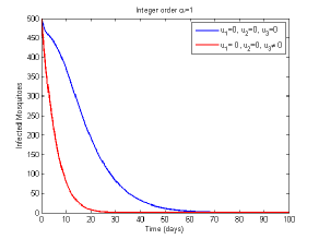
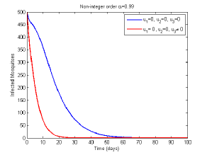
Figure 10: Numerical solutions of infected mosquitoes with insecticide spray control for $\alpha=1,0.99,0.95,0.90$

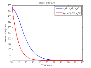
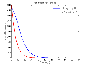
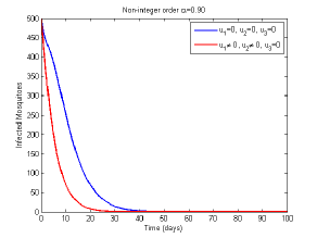
Figure 11: Numerical solutions of infected mosquitoes with treated bednets and treatment controls for $\alpha=1,0.99,0.95,0.90$

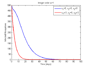
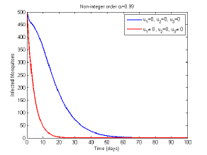
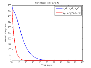
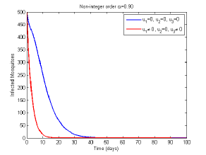
Figure 12: Numerical solutions of infected mosquitoes with treated bednets and insecticide spray controls for $\alpha=1,0.99,0.95,0.90$

Figure 13: Numerical solutions of infected mosquitoes with treatment and insecticide spray controls for $\alpha=1,0.99,0.95,0.90$

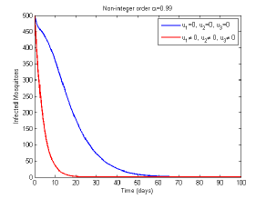
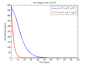
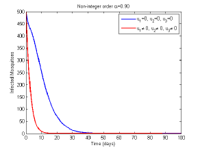
Figure 14: Numerical solutions of infected mosquitoes with all the three time dependent controls (treated bednets, treatment and insecticide spray) for $\alpha=1,0.99,0.95,0.90$

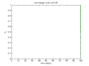
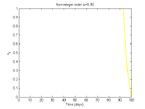
Figure 15: Optimal control function $u_{1}$ for $\alpha=1,0.99,0.95,0.90$

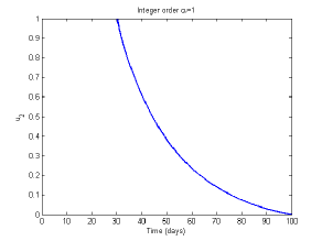
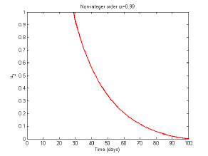
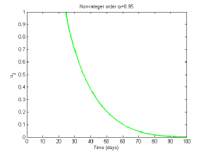
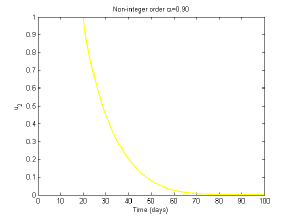
Figure 16: Optimal control function $u_{2}$ for $\alpha=1,0.99,0.95,0.90$

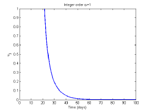
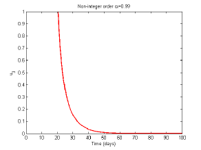
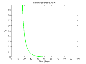
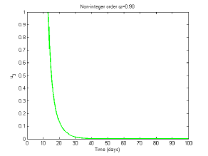
Figure 17: Optimal control function $u_{3}$ for $\alpha=1,0.99,0.95,0.90$

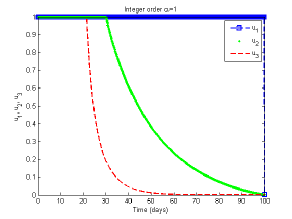
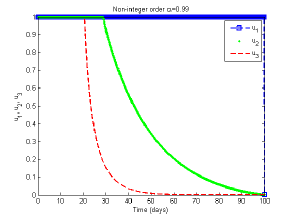
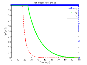
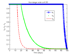
Figure 18: Optimal control functions $u_{1},\ u_{2}$ and $u_{3}$ for $\alpha=1,0.99,0.95,0.90$

5 Conclusion

This work considered an optimal control epidemiological model for malaria infection formulated in the sense of Caputo derivatives. The optimality of the fractional optimal control problem was solved using the forward-backward sweep method and the generalized euler method. We have numerically shown that when any of the time dependent controls or any combination of them are applied, the infected populations for both human and mosquitoes are reduced. Furthermore, when all the time dependent controls are used in the simulations, the reductions in the infected populations are more than any other control and prevention strategies. Our numerical solutions for the optimal control problem with fractional orders are much better than the integer order.

References

- Abdullahi et al. (2013) M. B. Abdullahi, Y. A. Hasan, and F. A. Abdullah. A mathematical model of malaria and the effectiveness of drugs. Applied Mathematical sciences, 7:3079–3095, 2013.
- Agrawal (2004) O. P. Agrawal. A general formulation and solution scheme for fractional optimal control problems. Nonlinear Dynamics, 38:323–337, 2004.
- Agrawal (2008a) O. P. Agrawal. A formulation and numerical scheme for fractional optimal control problems. Journal of Vibration and Control, 14:1291–1299, 2008a.
- Agrawal (2008b) O. P. Agrawal. A quadratic numerical scheme for fractional optimal control problems. Journal of Dynamic Ssystems, Measurement, and Control, 130, 2008b.
- Agrawal and Baleanu (2007) O. P. Agrawal and D. Baleanu. A hamiltonian formulation and a direct numerical scheme for fractional optimal control problems. Journal of Vibration and Control, 13:1269–1281, 2007.
- Agrawal et al. (2010) O. P. Agrawal, O. Defterli, and D. Baleanu. Fractional optimal control problems with several state and control variables,. Journal of Vibration and Control, 16:1967–1976, 2010.
- Athithan and Ghosh (2015) S. Athithan and M. Ghosh. Stability analysis and optimal control of a malaria model with larvivorous fish as biological control agent. Appl. Math. Inf. Sci., 9:1893–1913, 2015.
- Augsto et al. (2012) F. B. Augsto, N. Marcus, and K. O. Okosun. Application of optimal control to the epidemiology of malaria. Electronic Journal of DifferentialEquations, 2012:1–22, 2012.
- Bakhtiar (2016) T. Bakhtiar. Optimal intervention strategies for cholera outbreak by education and chlorination. Earth and Environmental Science, 31, doi:10.1088/1755-1315/31/1/012022, 2016.
- Basir et al. (2015) F. A. Basir, A. M. Elaiw, D. Kesh, and P. K. Roy. Optimal control of a fractional-order enzyme kinetic model. Control and Cybernetics, 44:1–18, 2015.
- Blayneh et al. (2009) K. Blayneh, Y. Cao, and H.-D. Kwon. Optimal control of vector-borne diseases: Treatment and prevention. Discrete and continuous dynamical systems series B, 11:587–611, 2009.
- Bonyah et al. (2016) E. Bonyah, K. Badu, and S. K. Asiedu-Addo. Optimal control application to an ebola model. Asian Pacific Journal of Tropical Biomedicine, 6(4):283–289, 2016.
- Chitnis et al. (2006) N. Chitnis, J. M. Cushing, and J. M. Hyman. Bifurcation analysis of a mathematical model for malaria transmission. SIAM J. Appl. Math, 67:24–45, 2006.
- Choi et al. (2015) S. Choi, E. Jung, and S-M. Lee. Optimal intervention strategy for prevention tuberculosis using a smoking-tuberculosis model. Journal of Theoretical Biology, 380:256–270, 2015.
- Diethelm et al. (2002) K. Diethelm, N. J. Ford, and A. D. Freed. A predictor-corrector approach for the numerical solution of fractional differential equations. Nonlinear Dyamics, 29:3–22, 2002.
- Diethelm et al. (2004) K. Diethelm, N. J. Ford, and A. D. Freed. Detailed error analysis for a fractional adams method. Nonlinear Dyamics, 36:31–52, 2004.
- Ding et al. (2012) Y. Ding, Z. Wang, and H. Ye. Optimal control of a fractional-order hiv-immune system with memory. IEEE Trans. Contr. Sys. Techn., 13:763–769, 2012.
- Frederico and Torres (2008) G. S. F. Frederico and D. F. M. Torres. Fractional conservation laws in optimal control theory. Nonlinear Dynamics, 53:215–222, 2008.
- Grigorieva and Khailov (2015) E. V. Grigorieva and E. N. Khailov. Optimal intervention strategies for a seir control model of ebola epidemics. Mathematics, 3, doi:10.3390/math3040961:961–983, 2015.
- Keegan and Dushoff (2013) L. T. Keegan and J. Dushoff. Population-level effects of clinical immunity to malaria. BMC Infectious Diseases 2013, 13:428, 2013.
- Kim et al. (2013) B. N. Kim, K. Nah, C. Chu, S. U. Ryu, Y. H. Kang, and Y. Kim. Optimal control strategy of plasmodium vivax malaria transmission in korea. Osong Public Health Res Perspect, 3:128–136, 2013.
- Lashari and Zaman (2012) A. A. Lashari and G. Zaman. Optimal control of a vector borne disease with horizontal transmission. Nonlinear Analysis: Real World Applications, 13:203–212, 2012.
- Lashari et al. (2012) A. A. Lashari, S. Aly, K. Hattaf, G. Zaman, I. H. Jung, and Xue-Zhi. Li. Presentation of malaria epidemics using multiple optimal controls. Journal of Applied Mathematics, 2012, Article ID 946504:17, 2012.
- Lenhart and Workman (2007) S. Lenhart and J. T. Workman. Optimal control applied to biological models. London, New York: Chapman and Hall, 2007.
- Magombedze et al. (2011) G. Magombedze, W. Gariraa, E. Mwenjeb, and C. P. Bhunua. Optimal control for hiv-1 multi-drug therapy. International Journal of Computer Mathematics, 88:314–340, 2011.
- Mandal et al. (2011) S. Mandal, R. R. Sarkar, and S. Sinha. Mathematical models of malaria - a review. Malaria Journal, 10:202, 2011.
- Moualeu et al. (2015) D. P. Moualeu, M. Weiser, R. Ehring, and P. Deuflhard. Optimal control for a tuberculosis model with undetected cases in cameroon. Commun Nonlinear Sci Numer Simulatt, 20:986–1003, 2015.
- Mwanga et al. (2014) G. G. Mwanga, S. Aly, H. Haario, and B. K. Nannyonga. Optimal control of malaria model with drug resistance in presence of parameter uncertainty. Applied Mathematical Sciences, 8:2701 – 2730, 2014.
- Ngonghala et al. (2012) C. N. Ngonghala, G. A. Ngwa, and M. I. Teboh-Ewungkem. Periodic oscillations and backward bifurcation in a model for the dynamics of malaria transmission. Mathematical Biosciences, 240:45–62, 2012.
- Okosun and Makinde (2011) K. O. Okosun and O. D. Makinde. Modelling the impact of drug resistance in malaria transmission and its optimal control analysis. International Journal of the Physical Sciences, 6:6479–6487, 2011.
- Okosun and Makinde (2013) K. O. Okosun and O. D. Makinde. Optimal control analysis of malaria in the presence of non-linear incidence rate. Appl. Comput. Math., 12:20–32, 2013.
- Okosun and Makinde (2014) K. O. Okosun and O. D. Makinde. A co-infection model of malaria and cholera diseases with optimal control. Mathematical Biosciences, 258:19–32, 2014.
- Okosun et al. (2013) K. O. Okosun, O. Rachid, and N. Marcus. Optimal control strategies and cost-effectiveness analysis of malaria model. BioSystems, 111:83–101, 2013.
- Okyere et al. (2016) E. Okyere, F. T. Oduro, S. K. Amponsah, I. K. Dontwi, and N. K. Frempong. Fractional order malaria model with temporary immunity. arXiv:1603.06416v1, 2016.
- Otieno et al. (2016) G. Otieno, J. K. Koske, and J. M. Mutiso. Cost effectiveness analysis of optimal malaria control strategies in kenya. Mathematics doi:10.3390/math4010014, 4, 2016.
- Petras (2011) I. Petras. Fractional-Order Nonlinear Systems: Modeling, Analysis and Simulation. Springer, 2011.
- Pinto and Machado (2013) C. M. A. Pinto and J. A. T. Machado. Fractional model for malaria transmission under control strategies. Computers and Mathematics with Applications., 66:908–916, 2013.
- Podlubny (1999) I. Podlubny. Fractional Differential Equations. Academic Press, New York, 1999.
- Pooseh et al. (2014) S. Pooseh, R. Almeida, and D. F. M. Torres. Fractional order optimal control problems with free terminal time. Journal of industrial and management optimization, 10:363–381, 2014.
- Rachah and Torres (2016) A. Rachah and D. F. M. Torres. Dynamics and optimal control of ebola transmission. Math.Comput.Sci., DOI 10.1007/s11786-016-0268-y, 2016.
- Ross (1911) R. Ross. The prevention of malaria. John Murray, London, 1911.
- Silva and Torres (2013) C. J. Silva and D. F. M. Torres. An optimal control approach to malaria prevention via insecticide-treated nets. Conference Papers in Mathematics, 2013, Article ID 658468:8, 2013.
- Sweilam and Al-Mekhlafi (2016) N. H. Sweilam and S. M. Al-Mekhlafi. On the optimal control for fractional multi-strain tb model. Optim. Control Appl. Meth. DOI: 10.1002/oca.2247, 2016.
- Tricaud and Chen (2010) C. Tricaud and Y. Chen. Time-optimal control of systems with fractional dynamics. International Journal of Differential Equations, 2010, Article ID 461048:16, 2010.
- Tumwiine et al. (2007a) J. Tumwiine, J. Y. T. Mugisha, and L. S. Luboobi. On oscillatory pattern of malaria dynamics in a population with temporary immunity. Computational and Mathematical Methods in Medicine, 8:191–203, 2007a.
- Tumwiine et al. (2007b) J. Tumwiine, J. Y. T. Mugisha, and L. S. Luboobi. A mathematical model for the dynamics of malaria in a human host and mosquito vector with temporary immunity. Applied Mathematics and Computation, 189:1953–1965, 2007b.