On the Minimum Mean -th Error in Gaussian Noise Channels and its Applications
Alex Dytso, Ronit Bustin, Daniela Tuninetti, Natasha Devroye, H.Vincent Poor, Shlomo Shamai (Shitz)
Alex Dytso, Daniela Tuninetti and Natasha Devroye are with the department of Electrical and Computer Engineering, University of Illinois at Chicago, IL, Chicago 60607, USA (e-mail: odytso2, danielat, devroye @ uic.edu).
Ronit Bustin is with the department of Electrical Engineering - Systems, Tel Aviv University, Tel Aviv, Israel (email:ronitbustin@post.tau.ac.il).
H.Vincent Poor is with the department of Electrical Engineering, Princeton University, NJ, Princeton 08544, USA (email:poor@princeton.edu).
S. Shamai (Shitz) is with the Department of Electrical Engineering,
Technion-Israel Institute of Technology, Technion City, Haifa 32000,
Israel (e-mail: sshlomo@ee.technion.ac.il). The work of Alex Dytso, Daniela Tuninetti and Natasha Devroye was partially funded by NSF under award 1422511. The work of Ronit Bustin was supported in part by the women postdoctoral scholarship of Israel’s Council for Higher Education (VATAT) 2014-2015. The work of H. Vincent Poor and Ronit Bustin was partially supported by NSF under awards CCF-1420575 and ECCS-1343210. The work of Shlomo Shamai was supported by the Israel Science Foundation (ISF). The contents of this article are solely the responsibility of the authors and do not necessarily represent the official views of the funding agencies. This work was presented in part at the 2016 IEEE International Symposium on Information Theory, Barcelona, Spain, and in part at the 2016 IEEE Information Theory Workshop, Cambridge, UK.
Abstract
The problem of estimating an arbitrary random vector from its observation corrupted by additive white Gaussian noise, where the cost function is taken to be the Minimum Mean -th Error (MMPE), is considered.
The classical Minimum Mean Square Error (MMSE) is a special case of the MMPE.
Several bounds, properties and applications of the MMPE are derived and discussed.
The optimal MMPE estimator is found for Gaussian and binary input distributions. Properties of the MMPE as a function of the input distribution, Signal-to-Noise-Ratio (SNR) and order are derived. In particular, it is shown that the MMPE is a continuous function of and SNR. These results are possible in view of interpolation and change of measure bounds on the MMPE.
The ‘Single-Crossing-Point Property’ (SCPP) that
bounds the MMSE for all SNR values above a certain value, at which the MMSE is known, together with the I-MMSE relationship is a powerful tool in deriving converse proofs in multi-user information theory. By studying the notion of conditional MMPE, a unifying proof (i.e., for any ) of the SCPP is shown. A complementary bound to the SCPP is then shown, which bounds the MMPE for all SNR values below a certain value, at which the MMPE is known.
As a first application of the MMPE, a bound on the conditional differential entropy in terms of the MMPE is provided, which then yields a generalization of the Ozarow-Wyner lower bound on the mutual information achieved by a discrete input on a Gaussian noise channel.
As a second application, the MMPE is shown to improve on previous characterizations of the phase transition phenomenon that manifests, in the limit as the length of the capacity achieving code goes to infinity, as a discontinuity of the MMSE as a function of SNR.
As a final application, the MMPE is used to show new bounds on the second derivative of mutual information, or the first derivative of the MMSE, that tighten previously known bounds important in characterizing the bandwidth-power trade-off in the wideband regime.
I Introduction
In the Bayesian setting the Minimum Mean Square Error (MMSE) of estimating a random variable from an observation is understood as a cost function111 Another common term used is a risk function. with a quadratic loss function (i.e., norm):
(1a)
(1b)
Another commonly used cost function is the norm with loss function given by the absolute value of the error (i.e., the difference between the variable of interest and its estimate). In general, cost functions with non-quadratic loss functions are not well understood and have been considered only for special cases, such as under the assumption of Gaussian statistics.
The interplay between estimation theoretic and information theoretic measures has been very fruitful; for example the so called I-MMSE relationship [1], that relates the derivative of the mutual information with respect to the Signal-to-Noise-Ratio (SNR) to the MMSE, has found numerous applications through out information theory [2]. The goal of this work is to show that the study of estimation problems with non-quadratic loss functions can also offer new insights into classical information theoretic problems. The program of this paper is thus to develop the necessary theory for a class of loss functions, and then apply the developed tools to information theoretic problems.
I-APast Work
The popularity of the MMSE stems from its analytical tractability, which is rooted in the fact that the MMSE is defined through the norm in (1b). The norm, in turn, allows applications of the well understood Hilbert space theory [3]. In information theoretic applications the norm is used, for example, to define an average input power constraint. The connection between the power constraint and the norm leads to a continuous analog of Fano’s inequality that relates the conditional differential entropy and the MMSE [4, Theorem 8.6.6].
Recently, in view of the I-MMSE relationship [1], the MMSE (in an Additive White Gaussian Noise (AWGN) channel) has received considerable attention. For example, in [5] the I-MMSE relationship was used to give a simple alternative proof of the Entropy Power Inequality (EPI) [6]. Moreover, the so called ‘Single-Crossing-Point Property’ (SCPP) [7, 8] that bounds the MMSE for all SNR values above a certain value at which the MMSE is known, together with the I-MMSE relationship, offers an alternative, unifying framework for deriving information theoretic converses, such as:
[7] to provide an alternative proof of the converse for the Gaussian broadcast channel (BC) and show a special case of the EPI;
in [9] to provide a simple proof for the information combining problem and a converse for the BC with confidential messages;
in [8], by using various extensions of the SCPP,
to prove a special case of the vector EPI, a converse for the capacity region of the parallel degraded BC under per-antenna power constraints and under an input covariance constraint, and a converse for the compound parallel degraded BC under an input covariance constraint; and
in [10] to provide a converse for communication under an MMSE disturbance constraint.
In [11] we demonstrated a bound that complements the SCPP, that bounds the MMPE for all SNR values below a certain value at which the MMSE is known, and allows for a finer characterization of the phase transition phenomenon that manifests as a discontinuity of the MMSE as a function of SNR, as the length of the codeword goes to infinity. This plays an important role in characterizing achievable rates of the capacity achieving codes [12] and [13]. One of the applications of the tools presented in this work is an improvement on the bound in [11, Theorem 1].
Many other properties of the MMSE in relation to the I-MMSE have been studied in [7, 14, 15, 16]. For a comprehensive survey on results, applications and extensions of the I-MMSE relationship we refer the reader to [9].
While the MMSE has received considerable attention and is well understood, non-quadratic cost functions are only understood in special cases, such as under the assumption of Gaussian statistics. For example, in [17] it was shown that under scalar Gaussian statistics, for a large class of symmetric loss functions the optimal linear MMSE (LMMSE) estimator is also optimal. The result of [17] was extended in [18] to a large class of cost functions that also include asymmetric loss functions. Other early work in this direction includes also [19].
In [20], the authors studied the expected norm of the error,
when the input is assumed to be a Gaussian mixture. The authors showed that, as the dimension of the signal goes to infinity, the optimal LMMSE estimator minimizes the expected maximum error.
In [21] and [22] the authors studied a class of even and nondecreasing and even and convex loss functions and gave a sufficient condition on the conditional distribution of the input given the output , so that the conditional expectation is the optimal estimator.
In [23], the authors studied a scalar additive noise channel and an cost function and showed a necessary and sufficient condition on the noise and the input distributions to guarantee that the optimal estimator is linear. Moreover, if the source and noise variances are the same, then the optimal estimator is linear if and only if input and the noise distributions are identical.
In [24] and [25] the authors considered the problem of transmitting a modulated signal over a discrete memoryless channel where the performance criterion was taken to be the cost function.
To that end, the authors showed tight exponential bounds for very small and very large values of .
In [26] the authors focused on designing an appropriate cost function such that the output of the trained model approximates the desired summary statistics, such as the conditional expectation, the geometric mean or the variance.
In non-Bayesian estimation cost functions have been considered in [27] and [28], in a context of minimax estimation, and the authors gave lower and upper bounds on the exponential behavior of the cost function. For a non-Bayesian treatment of non-quadratic cost functions we refer the reader to [29].
Looking into non-quadratic cost functions is further motivated by the fact that often the quadratic cost function may not be the correct measure of signal fidelity for certain applications. This is especially true in image processing where error metrics, more sensitive to structural changes of the input signal, better capture human perceptions of quality. We refer the reader to [30] for a survey of recent results in this direction.
I-BPaper Outline and Main Contributions
In this work we are interested in studying a cost function, termed the Minimum Mean -th Error (MMPE)222 The abbreviation MMPE has been used before in [9, Chapter 8] for the Minimum Mean Poisson Error. , the scalar version of which is given by
(2a)
(2b)
where the infimum is over all estimators .
Our contributions are as follows:
1.
In Section II we formally define the vector version of the MMPE in (2) and introduce related definitions.
2.
In Section III we study properties of the optimal MMPE estimator and show:
•
In Section III-A, Proposition 1 shows that the MPPE optimal estimator indeed exists;
•
In Section III-B, Proposition 2 derives an orthogonality-like principle that serves as a necessary and sufficient condition for an estimator to be MMPE optimal;
•
Section III-C gives examples of optimal MMPE estimators. In particular, in Proposition 3 we find the MMPE for Gaussian random vectors, and in Proposition 4 for discrete binary random variables; and
•
In Section III-D, Proposition 5 shows some basic properties of the optimal MMPE estimator in terms of input distribution, such as, linearity, stability, degradedness, etc. Moreover, via an example it is shown that in general the MMPE optimal estimator is biased on average (i.e., the first moment of the error (bias) is not zero). However, it is shown that the -th order estimator is unbiased on average in sense that the -th moment of the error is zero.
3.
In Section IV we study properties of the MMPE as a function of order , SNR and the input distribution that will be useful in a number of applications:
•
In Section IV-A, Proposition 6 shows that the MMPE is invariant under translations of the input random vector and derives basic scaling properties;
•
In Section IV-B, Proposition 7 shows that, as far as estimation error over the channel is concerned the estimation of the input is equivalent to the estimation of the noise ; and
•
In Section IV-C, Proposition 8 gives a ‘change of measure’ result that allows one to take the expectation in the definition of the MMPE with respect to an output at a different SNR.
4.
In Section V we discuss basic bounds on the MMPE and show:
•
In Section V-A, Proposition 10 develops basic ordering bounds between MMPE’s of different orders and bounds equivalent to that of the LMMSE bound;
•
In Section V-B, Proposition 11 shows that, under an appropriate moment constraint on the input distribution, the Gaussian input is asymptotically the ‘hardest’ to estimate;
•
In Section V-C, Proposition 12 derives interpolation bounds for the MMPE. One of the consequences of such bounds is Proposition 13, which shows that the MMPE is a continuous function of order ; and
•
In Section V-D, Proposition 14 derives bounds on the MMPE with discrete vector inputs. This in turn leads to a result in Proposition 15 that shows that MMPE, similarly to the MMSE, can exhibit phase transitions (i.e., discontinuities as function of the SNR as dimension of the input goes to infinity).
5.
In Section VI we define the conditional MMPE and show:
•
Proposition 16 shows that conditioning reduces the MMPE; and
•
Proposition 17 shows that the MMPE estimation of from two AWGN observations is equivalent to estimating from a single observation with a higher SNR. This implies that the MMPE is a decreasing function of SNR.
6.
In Section VII we show applications of the developed tools:
•
In Proposition 18, by using the tools developed for the conditional MMPE, a simple proof of the SCPP for the MMSE is given, and extended to the MMPE;
•
In Proposition 19 we use the change of measure result in Proposition 8 to show a bound that complements the SCPP bound, that it is bounds the MMPE for all SNR values below a certain SNR value at which the MMPE is known; and
•
In Proposition 20, by using change of measure result in Proposition 19 and continuity of the MMPE in from Proposition 13, we show that for any finite dimensional input the MMPE is a continuos function of SNR.
7.
In Section VIII we apply the developed bounds and generalize or improve some well known information theoretic MMSE bounds:
•
In Section VIII-A, Theorem 1 gives a general inequality that bounds the conditional differential entropy via the MMPE of which the continuous analog of Fano’s from [4, Theorem 8.6.6] is a special case;
•
In Section VIII-B, Theorem 2 generalizes the Ozarow-Wyner bound [31] on the
mutual information achieved by a discrete input on an AWGN channel, to vector discrete inputs and yields the sharpest known version of this bound. Moreover, in Theorem 3 we show how the bound behaves as the dimension of the input goes to infinity;
•
In Section VIII-C, Theorem 4 improves on the previous characterizations of the width the phase transition
region of finite-length code of length given by in [11] to . This in turn also improves the converse result on the communications under disturbance constrained problem studied in [11]; and
•
In Section VIII-D, Proposition 21 we show
how the MMPE can be used to provide new lower and upper
bounds on the derivative of the MMSE.
I-CNotation
Throughout the paper we adopt the following notational conventions:
•
Deterministic scalar and vector quantities are denoted by lower case and bold lower case letters, respectively. Matrices are denoted by bold upper case letters;
•
Random variables and vectors are denoted by upper case and bold upper case letters, respectively, where r.v. is short for either random variable or random vector, which should be clear from the context;
•
If is a r.v. we denote the support of its distribution by ;
•
The symbol may denote different things: is the determinant of the matrix ,
is the cardinality of the set ,
is the cardinality of , or
is the absolute value of the real-valued ;
•
denotes the expectation operator;
•
We denote the covariance of r.v. by ;
•
denotes the density of a real-valued Gaussian r.v. with mean vector and covariance matrix ;
•
The identity matrix is denoted by ;
•
Reflection of the matrix along its main diagonal, or the transpose operation, is denoted by ;
•
The trace operation on the matrix is denoted by ;
•
The Order notation implies that is a positive semidefinite matrix;
•
denotes logarithms in base ;
•
is the set of integers from to ;
•
For we let
denote the largest integer not greater than ;
•
For we let and ;
•
Let be two real-valued functions.
We use the Landau notation to mean that for some there exists an such that for all ,
and to mean that for every there exists an such that for all ;
•
We denote the conditional r.v. as ;
•
We denote the upper incomplete gamma function and the gamma function by
(3a)
(3b)
The generalized Q-function is denoted by
(3c)
In particular, the generalized -function can be related to the standard -function, by using the relationship and , as ; and
•
We define the volume of the region embedded in as
(4)
In particular, the volume of the -dimensional ball of radius center at origin is given by
II Cost Function Definition
Motivated by the study of cost functions with non-quadratic error we define the following norm.
Definition 1.
For the r.v. and
(5)
For the function in (5) defines a norm and obeys the triangle inequality
(6)
as shown in Appendix A.
Therefore, throughout the paper
we define the space, for , as the space of r.v. on a fixed probability space such that the norm in (5) is finite. However, many of our results will hold for , for which (5) is not a norm.
and for uniform over the dimensional ball of radius the norm in (5) is given by
(8)
Note that for we have that and therefore from now on we will refer to as -th moment of . Naturally, for , there are many other ways for defining the moments, see for example [32]. However, in view of the information theoretic problems we are interested in, such for example from previous work [11], the definition in (5) arises naturally.
Definition 2.
We define the minimum mean -th error (MMPE) of estimating from as
(9a)
(9b)
and where the minimization is over all possible Borel measurable functions . Whenever the optimal MMPE estimator exists, we shall denote it by .333The restriction to measurable functions, in Definition 2, is necessary. See [33] for surprising complications that can arise without this assumption.
We shall denote
(10)
if and are related as
(11)
where , is independent of , and is the SNR. When it will be necessary to emphasize the SNR at the output , we will denote it with . Since the distribution of the noise is fixed
is completely determined by distribution of and and there is no ambiguity in using the notation . Applications to the Gaussian noise channel will be the main focus of this paper.
For , the MMPE reduces to the MMSE, that is, and .
Note that there are other ways of defining the loss function in (9); our definition in (9) is motivated by:
•
For the error in (9) reduces to a natural expression with loss function given by ;
•
The definition in (9) naturally appears in applications of Hölder’s or Jensen’s inequalities to ; and
•
The norm in (5) used in the definition of (9) can be related to information theoretic quantities, such as differential entropy and Reyni entropy, via the vector moment entropy inequality from [34].
We shall also look at the -th error achieved by the suboptimal (unless ) estimator , that is,
(12)
which represents higher order moments of the MMSE loss function and serves (see below) as an upper bound on (9).
III Properties of the Optimal MMPE Estimator
III-AExistence of Optimal Estimator
It is important to point out that in general is not equal to the MMPE, as might not be the optimal estimator under the -th norm. The first result of this section shows that for AWGN channel the optimal estimator indeed exists.
Proposition 1.
For , , the optimal estimator is given by the following point-wise relationship
A result similar to that in Proposition 1 can be found in [29, Theorem 4.1.1] where it has been shown that for a given an estimator is optimal provided that the minimum on the right hand side of (13) exists. In contrast to [29, Theorem 4.1.1], Proposition 1 shows that the minimum in (13) exists for any , and is the MMPE optimal estimator for any .
Proposition 1 immediately implies the following corollary on the interchange of the expectation and infimum which will be used in many of the following proofs.
for in (13).
Therefore, we have the following chain of inequalities
(15)
This concludes the proof.
∎
III-BOrthogonality-like Property
The MMPE for differs from MMSE
in a number of aspects. The main difference is that the norm defined in (5) is not a Hilbert space norm in general (unless ); as a result, there is no notion of inner product or orthogonality, and , unlike can no longer be thought of as an orthogonal projection. Therefore, the orthogonality principle—an important tool in the analysis of the MMSE—is no longer available when studying the MMPE for . However, an orthogonality-like property can indeed be shown for the MMPE.
Proposition 2.
(Necessary and Sufficient Condition for the Optimality of ).
For any , any , , is an optimal estimator if and only if
(16a)
for any deterministic function , that is,
(16b)
where .
Moreover, for the condition in (16a) is necessary for optimality.
Moreover, for Proposition 2 reduces to the familiar orthogonality principle
(19)
Remark 1.
In the analysis of the MMSE the orthogonality property is an important tool, used for example to show that is the unique minimizer. The argument goes as follows: assume that we have another optimal estimator , then by orthogonality principle,
(20)
By choosing we see that , arriving at a contradiction. This implies that is the unique estimator up to a set of measure zero.
In [23, Lemma 1], by replicating the above argument and by assuming that and , it was shown that the optimal MMPE estimator is unique. However, since the proof relies heavily on the assumption that and , this argument cannot be extended in a straightforward way to or .
However, uniqueness of the MMPE optimal estimator can be shown for (i.e., strictly convex loss functions) by using Proposition 1 in conjunction with [29, Corollary 4.1.4].
III-CExamples of Optimal MMPE Estimators
In general we do not have a closed form solution for the MMPE optimal estimator in (13).
Interestingly, the optimal estimator for Gaussian inputs can be found and is linear for all . Note that similar results have been demonstrated in [17] and [23] for scalar Gaussian inputs. Next we extend this result to vector inputs and give two alternative proofs of the linearity of the optimal MMPE estimator for Gaussian inputs, via Proposition 1 and via Proposition 2.
Proposition 3.
For input and
(21a)
with optimal estimator given by
(21b)
Proof.
The proof follows by observing that has a Gaussian distribution and is independent of . So, for any two functions and we have
(22)
Therefore, by using (22) for estimator the necessary and sufficient conditions in Proposition 2 hold and thus the linear estimator must be an optimal one. Finally observe that
(23)
where we have used .
For a proof that uses only Proposition 1 see Appendix D.
∎
The optimal MMPE estimator is in general a function of as shown next.
Proposition 4 will be useful in demonstrating several examples and counter examples in the following sections. Note that for the practically relevant case of BPSK modulation, or the optimal estimator in (24a) reduces to
(25a)
which for is the hard decision decoder
(25d)
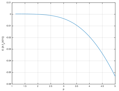
By Proposition 4 we can show that the orthogonality principle only holds for (when MMPE corresponds to MMSE) as shown in Fig. 1(a), where we plot vs. for BPSK input and observe it is zero only for .
(Average Bias of the MMPE optimal Estimator)
An estimator is said to be unbiased on average if
In general is unbiased on average only for , since
(26)
Fig. 1(b) shows that in general the optimal MMPE estimator is biased on average;
it plots vs. for and , with as in Proposition 4. This comes as no surprise as it is very common in Bayesian estimation that the optimal estimator is biased [35].
However, the optimal MMPE estimator is unbiased in the sense that the -th moment of the bias is zero. This can be seen from the orthogonality like property in Proposition 2 by taking to be the vector of all one’s
(27)
IV Properties of the MMPE
In this section we explore properties of the MMPE as a function of SNR and of the input distribution.
IV-ABasic Properties
The next two properties of the MMPE directly follow from the properties of in Proposition 5.
Proposition 6.
For any
(28a)
(28b)
Proposition 6 implies that the MMPE, like the MMSE, is invariant under translations, and that scaling the input results in scaling the SNR and the error.
IV-B Estimation of the Input is Equivalent to Estimation of the Noise
The following lemma is commonly applied in the analysis of the MMSE.
This shows the equality in (30a).
Moreover, since exists and the infimum in (31) is attainable by Proposition 1, so is the infimum in (32). Therefore, from (32) we have that exists and is given by
The next result enables us to change the expectation from to in (9) whenever . This is particularly useful when we know the MMPE, or the structure of the optimal MMPE estimator, at one SNR value but not at another smaller SNR value.
One must be careful when evaluating Proposition 8.
For example, since we have that
at first glance it appears that the expectation on the right of (35) is zero while is not, thus
violating the equality.
However, a more careful examination shows that when the limit and expectation in (35) cannot be exchanged; indeed we have that
where in the last equality we used the
moment generating function of the Cauchy r.v. .
As an example, Proposition 8 for
with the optimal linear estimator from Proposition 3, i.e., for some ,
evaluates to
where the equalities follow from:
a) linearity of expectation and the fact that and are independent; and
b) since and and by choosing in order to minimize the expression in a).444Note that this optimal is evident from the specific change of measure that we have used. Instead of having the estimator according to Proposition 3 as we get it with the normalization by .
V Bounds on The MMPE
In this section we develop bounds on the MMPE, many of which generalize well known MMSE bounds. However, we also show bounds that are unique to the MMPE and emphasize the usefulness of the MMPE.
V-AExtension of Basic MMSE Bounds
An important upper bound on the MMSE often used in practice is the LMMSE.
It is interesting to point out that in the derivation of the bounds in Proposition 10 no assumption is put on the distribution of , and thus the bounds hold in great generality.
If is composed of independent identically distributed (i.i.d.) Gaussian elements, then the moment in Proposition 10 can be tightly approximated in terms of factorials as
(38)
which is tight for even and integer .
It is not difficult to check that for Proposition 10 reduces to Proposition 9.
The reason that the bounds on are only available for , while the bounds on are available for , is because the proof of the bound in (37b) uses Jensen’s inequality, which requires , while the proof of the bound in (37d) does not.
V-BGaussian Inputs are the Hardest to Estimate
Note that the bounds in Proposition 10 are similar to the bound in (36a) and blow up at . Therefore, it is desirable to have bounds as in (36b). The next result demonstrates such a bound and shows that Gaussian inputs are asymptotically the hardest to estimate.
Proposition 11.
For , , and a random variable such that , we have
(39a)
where
for :
(39b)
for :
(39c)
Moreover, a Gaussian with per-dimension variance (i.e., ) asymptotically achieves the bound in (39a), since .
One of the key advantages of using the MMPE is that the MMPE of order can be tightly predicted based on the knowledge of the MMPE at lower orders and higher orders .
At the heart of this analysis is the interpolation result of spaces [36]:
given and such that , the -th norm can be bounded as
(40)
which implies that the norm is log-convex
and thus a continuous function of [37, Theorem 5.1.1].
Next, we present several interpolation results for the MMPE.
Proposition 12.
(Log-Convexity and Interpolation.)
For any and such that
(41a)
where , we have for any
(41b)
In particular,
(41c)
Moreover,
(41d)
In particular,
(41e)
(41f)
Proof.
The bound in (41b) follows by applying (40)
with . The bounds in (41c) follow by choosing .
where the last inequality follows from (40) by choosing .
Finally, the bounds in (41e) and (41f) follow by choosing in (41d) equal to and respectively. This concludes the proof.
∎
From log-convexity we can deduce continuity.
Proposition 13.
(Continuity.)
For any and , and are continuous functions of .
Proof.
Continuity of follows from log-convexity in (41c) while the continuity of MMPE follows from
where the last inequality is due to the continuity of the norm.
∎
An interesting question is whether the following interpolation inequality holds:
(43)
instead of (41e) and (41f).
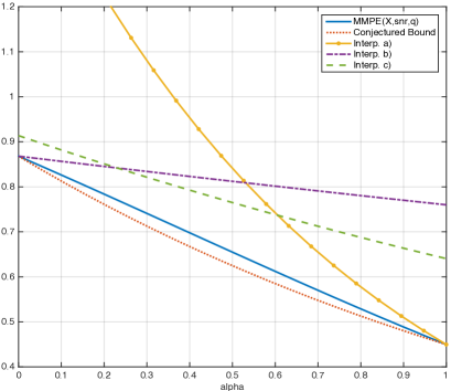
A counter example to the interpolation inequality in (43) is shown in Fig. 2 where we take a binary input equality likely, , and and show:
•
The MMPE of of order versus where is computed according to (41a) (blue-solid line);
•
The interpolation bound in (41e) (purple dashed-dotted line);
•
The interpolation bound in (41f) (yellow solid-dotted line);
•
The interpolation bound in (41d) with (green dashed line); and
•
The right-hand side of the conjectured inequality in (43) (red-dotted line).
Figure 2: Interpolation bounds from Proposition 12 and the conjectured bound in (43) versus . Clearly the conjectured bound is below the true MMPE thus (43) cannot be true.
V-DBounds on Discrete Inputs
So far, by using Proposition 10, we have shown that the MMPE as a function of decreases as . Next we show that the MMPE can decrease exponentially in . Such a behavior has been already observed for the MMSE in [38] and [15].
The exponential behavior of the MMPE of discrete inputs can be clearly seen for the case as follows. By using we have that
(45)
where the last inequality follows from the Chernoff’s bound .
Having developed bounds on the MMPE of discrete inputs, we are now in the position to demonstrate a phase transition phenomenon, that is, we show that as the MMPE becomes a discontinuous function of the SNR.
Proposition 15.
For (i.e., vector of all one’s or all minus ones) equally likely then
for any and , by using Proposition 14 we have that
(51)
and, in light of the limit in (50),
we have that the bound in (48) holds.
This concludes the proof.
∎
VI Conditional MMPE
We define the conditional MMPE as follows.
Definition 3.
For any and , the conditional MMPE of given is defined as
(52)
The conditional MMPE in (52) reflects the fact that the optimal estimator has been given additional information in the form of .
Note that when is independent of we can write the conditional MMPE for as
(53)
Since giving extra information does not increase the estimation error, we have the following result.
Proposition 16.
(Conditioning Reduces the MMPE.)
For every , and random variable , we have
(54)
Finally, the following Proposition generalizes [9, Proposition 3.4] and states that the MMPE estimation of from two observations is equivalent to estimating from a single observation with a higher SNR.
Proposition 17.
For every and , let where and where are mutually independent. Then
(55)
Proof.
For two independent observations
and
where and are independent, by using maximal ratio combining, we have that
where . Next by using the same argument as in [9, Proposition 3.4], we have that the conditional probabilities are
(56)
for . The equivalence of the posterior probabilities implies that the estimation of from is as good as the estimation of from . This concludes the proof.
∎
Propositions 17 and Proposition 16 imply that, for fixed and
(57)
and we have the following:
Corollary 2.
is a non-increasing function of .
VII Advance Bounds: SCPP Bound and Its Complement
The SCPP is a powerful too that can be used to show the advantage of Gaussian inputs over arbitrary inputs in certain channels with Gaussian noise. In conjunction with the I-MMSE relationship, the SCPP provides simple and insightful converse proofs to the capacity of multi-user AWGN channels. The original proof of the SCPP in [7] and [8] relied on bounding the MMSE. Next we give a simpler proof of the SCPP that does not require knowledge of the derivative the MMSE and can easily be extended to the MMPE of any order .
First observe that, in light of the bound in (37d), for any we can always find a such that
(58)
Next we generalize the SCPP bound to the MMPE.
Proposition 18.
Let for some . Then
(59a)
where
(59b)
Proof.
Let for and let
Then
where . Next, let
(60)
and define a suboptimal estimator given as
(61)
for some to be determined later. Then
and
(62)
where the (in)-equalities follow from:
a) Proposition 17;
b) by using the sub-optimal estimator in (61); and
c) by choosing for defined in (60).
Next, by applying the triangle inequality to (62) we get
(63)
(64)
(65)
where in the last step we used .
Note that for the case , instead of using the triangular inequality in (63), the term in (62) can be expanded into a quadratic equation for which it is not hard to see that the choice of is optimal and leads to the bound
The proof is concluded by noting that .
∎
Remark 3.
We conjecture that the multiplicative constant can be sharpened to for all . However, in order to make such a claim one must solve the following optimization problem
(66)
where and are independent and . Because it is not clear how to solve (66) for and thus we leave it for the future work.
Remark 4.
Note that the proof of Proposition 18 does not require the assumption that is Gaussian and only requires the assumptions of Proposition 17. That is, we only require that a channel is such that the estimation of from two observations is equivalent to estimating from a single observation with a higher SNR.
VII-AComplementary SCPP bound
In this section we give a bound that complements the SCPP bound, that is, while the SCPP bounds the MMPE for all , we give a bound that bounds the MMPE for all where it is assumed that the MMPE is known at .
The next result enables us to bound the MMPE at with values of the MMPE at while varying the order.
where the (in)-equalities follow from: a) Hölder’s inequality with conjugate exponents such that ; and b) by recognizing that the expectation of the exponential is the moment generating function of a Chi-square distribution of degree , which exists only if .
Next, we let and let in (67), so that
. Observe that now the bound in (67) holds for all values of since
The bound in Proposition 19 is the key in showing new bounds on the phase transitions region for the MMSE, presented in the next section.
As an application of Proposition 19 we show that the MMPE is a continuous function of SNR.
Proposition 20.
For fixed and , is a continuous function of .
Proof.
Assume without loss of generality that
where the (in)-equalities follow from: a) since the MMPE is a decreasing function of SNR and since ; b) by using Proposition 19; and c) by definition of in Proposition 19 we have that and , and by continuity of the MMPE in from Proposition 13.
This concludes the proof.
∎
VIII Applications
We next show how the MMPE can be used to derive tighter versions of some well known bounds. It is important to point out that even though the focus of this paper is on the AWGN setting, the results that follow (Theorem 1, Theorem 2 and Theorem 3) apply to any additive channel model in which the noise is an absolutely continuous random variable, without the need for the i.i.d. assumption.
VIII-ABounds on the Differential Entropy
For any random vector such that and any random vector ,
the following inequality is considered to be a continuous analog of Fano’s inequality [4]:
(69)
(70)
where the inequality in (70) is a consequence of the arithmetic-mean geometric-mean inequality, that is, for any we have used
where ’s are the eigenvalues of .
By applying (70) to the AWGN setting, for any such that by using Proposition 10 with , we can arrive at the trivial bound: for any
(71)
Next, we show that
the inequality in (70) can be generalized in terms of the norm in (5), and
the trivial bound in (71) can be improved.
Theorem 1.
For any such that and for some , and for any , we have
Note that the result in Theorem 1 holds in great generality, i.e., the AWGN assumption is not necessary. As an application of Theorem 1 to the AWGN setting we have the following stronger version of the inequality in (71).
The proof follows by setting and in the statement of Theorem 1.
∎
VIII-BGeneralized Ozarow-Wyner Bound
In [31] the following “Ozarow-Wyner lower bound” on the mutual information achieved by a discrete input
transmitted over an AWGN channel was shown:
(74a)
(74b)
where is the LMMSE.
The advantage of the bound in (74) compared to existing bounds is its computational simplicity.
The bound on the in (74) has been sharpened in [40, Remark 2] to
(75)
since .
Next, we generalize the bound in (74) to discrete vector inputs and give the sharpest known bound on the gap term.
Theorem 2.
(Generalized Ozarow-Wyner Bound)
Let be a discrete random vector with finite entropy, such that , and , and let be a set of continuous random vectors, independent of , such that for every , , and
It is interesting to note that the lower bound in (76b) resembles the bound for lattice codes in [41, Theorem 1], where can be thought of as dither, corresponds to the log of the normalized -moment of a compact region in , corresponds to the log of the normalized MMSE term, and corresponds with the capacity .
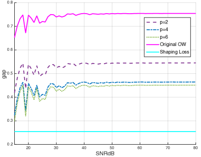
In order to show the advantage of Theorem 2 over the original Ozarow-Wyner bound (case of and with LMMSE instead of MMPE), we consider uniformly distributed with the number of points equal to , that is, we choose the number of points such that .
Fig. 3 shows:
•
The solid cyan line is the “shaping loss” for a one-dimensional infinite lattice and is the limiting gap if the number of points grows faster than ;
•
The solid magenta line is the gap in the original Ozarow-Wyner bound in (74); and
•
The dashed purple, dashed-dotted blue and dotted green lines are the new gap due to Theorem 2 for value of , respectively, and where we chose .
We note that the version of the Ozarow-Wyner bound in Theorem 2 provides the sharpest bound for the gap term.
An open question, for , is what value of provides the smallest gap and if that coincide with the ultimate “shaping loss”.
VIII-CNew bounds on the MMSE and Phase Transitions
The SCPP is instrumental in showing the behavior of the MMSE of capacity achieving codes. For example, as the length of any capacity achieving code goes to infinity, the MMSE behaves as follows:
(81)
as shown:
in [12], for the Gaussian point-to-point channel with the output with ;
in [13], for the Gaussian BC with outputs and , where and rate pair for some , with ;
in [13], for the Gaussian wiretap channel with outputs (primary) and (eavesdropper) with maximum equivocation and rate , for ;
and in [10], for the Gaussian point-to-point channel with output and an MMSE disturbance constraint at measured by for some with .
The jump discontinuities in (81) at and are referred to as the phase transitions.
Based on the above, an interesting question is how the MMSE in (81) behaves for codes of finite length. In [11], in order to study the phase transition phenomenon for inputs of finite length, the following optimization problem was proposed:
Definition 4.
(82a)
s.t.
(82b)
for some .
Investigation in [11] revealed that in (82a) must be of the following form:
for some and some function , where the region is referred to as the phase transition region and its width is defined as
In [11] the following was established for and :
(83)
and the width of phase transition region scales as
The main result of this subsection is shown next. It uses Propositions 19 and Proposition 12.
Theorem 4.
For ,
(84a)
where and
(84b)
(84c)
and where the minimizing in (84a) can be approximated by
(84f)
Moreover, the width of the phase transition region scales as
(84g)
Proof.
From the SCPP complementary bound in Proposition 19 with we have that
(85)
From the interpolation result in Proposition 12 letting , we have that for some such that and
By putting all of the bounds together, letting and observing that
we get the bound in (84a).
Finally, the proof of approximately optimal in (84f) is given in Appendix N.
∎
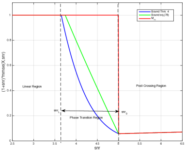
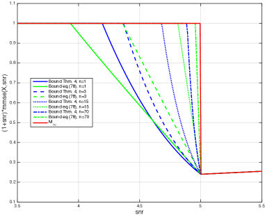
(a)For and . Here .
(b)For and . Several values of .
Figure 4: Bounds on vs .
The bounds in Theorem 4 and in (83) are shown in Fig. 4. The bound in Theorem 4 is asymptotically tighter than the one in (83). This follows since the phase transition region shrinks as for Theorem 4, and as for the bound in (83).
It is not possible in general to assert that Theorem 4 is tighter than (83).
In fact, for small values of , the bound in (83) can offer advantages, as seen for the case shown in Fig. 4(b). Another advantage of the bound in (83) is its analytical simplicity.
VIII-DBounds on the derivative of the MMSE
The MMPE can be used to study the second derivative of mutual information (or first derivative of MMSE), as initiated
for in [7] and for in [8], namely,
(87)
The second derivative of mutual information is important in characterizing the bandwidth-power trade-off in the wideband regime [42] and [43], and has also been used in the proof of the SCPP in [7] and [8]. Moreover, in [7] it has been shown that the derivative of the MMSE and the quantity in (12) are related by the following bound for :
(88)
The main result of this subsection is the next bound.
It can be observed that, for the case , by using the bound in (37b) from Proposition 10 we have that
(90)
which significantly reduces the constant in (88) from to .
For a similar but slightly different bound than that in (90) on please see [11].
IX Concluding Remarks
This paper has considered the problem of estimating a random variable from a noisy observation under a general cost function, termed the MMPE. We have show that many properties of the MMSE and the conditional expectation (i.e., optimal MMSE estimator) are identical or have a natural generalization to the MMPE and the MMPE optimal estimator.
We have also provided a new simpler proof of the SCPP for the MMSE and generalized it to the MMPE. We have shown that the new framework of the MMPE also permits the development of bounds that are complementary to the SCPP which in turn allows for new tighter characterizations of the phase transition phenomena that manifest, in the limit
as the length of the capacity achieving code goes to infinity, as a discontinuity of the MMSE as a function of SNR.
We have also shown connections between the MMPE and the conditional differential entropy by generalizing a well know continuous analog of Fano’s inequality.
The MMPE was further used to refine bounds on the conditional entropy and improve the gap term in the Ozarow-Wyner bound.
Currently, we are investigating the connections between bounds on the MMPE provided in this work and the rate distortion problem with the MMPE distortion measure. Possible future applications of the sharpened version of the Ozarow-Wyner bound include sharpening the bounds on discrete inputs in [44] and [45]. Another interesting future direction is to consider a modified ‘information bottleneck problem’ [46] where the constraint on the mutual information is replaced by a constraint on the MMPE.
Appendix A Proof of the Triangle Inequality in (6)
It is well know that the trace operator is an inner product in the space of matrices and since the inner product induces a norm we have
Therefore, we have that
where the inequalities follow from: a) triangle inequality for inner product induce norm for ; and b) Minkowski inequality for the expectation which holds for .
This concludes the proof.
For simplicity, we look at the case . The case for follows similarly. We first assume that .
The first direction follows trivially:
(91)
The other direction follows by using
(92)
where we focus on the inner expectation and show that the infimum is achieved by given in (13). Since is now given, we are simply looking for an optimal solution to the more general problem
(93)
where . The goal is to show that the infimum in (93) is achievable. Clearly, the infimum exists since
(94)
(95)
where the last inequality follows from [7, Proposition 6] which asserts that for any , is a sub-Gaussian random variable and hence all conditional moments are finite.
Next, we show that is a continuous function of . Recall, that any given function is continuous if implies as .
For arbitrary take a sequence such that , we want to show that
(96)
This can be done with the help of the dominated convergence theorem.
We must find an integrable random variable such that for all ; this is found as
(97)
(98)
where the inequalities follow from: a) which holds for any ; and b) recall that every convergent sequence is bounded and since the sequence converges to it is also bounded by some finite for every .
The integrability of follows again by the sub-Gaussian argument from [7, Proposition 6].
Therefore, we conclude that the function is continuous.
Next, we show that the infimum is attainable by some .
By definition of the infimum there exists some (not necessarily convergent) such that
(99)
Towards a contradiction, assume that . Then by Fatou’s lemma
(100)
However, this contradicts the result in (95) and therefore sequence must be bounded. This, together with the fact that is continuos, implies that the infimum is attainable and thus
(101)
Therefore, for each there exists that minimize the expression and the optimal estimator defined point-wise is given by
(102)
For the case of the problem reduces to
(103)
which is bounded if and only if .
This concludes the proof.
We take a classical approach used in estimation theory to find an optimal estimator by using tools from calculus of variations [47, Ch.7 Thm.1]. A necessary condition for to be a minimizer in (13) is expressed through a functional derivative as
(104)
for all admissible .
Therefore, we focus on the following limit:
(105)
We seek to apply the dominated convergence theorem to (105) in order to interchange the order of the limit and the expectation. To that end we let and
(106)
(107)
(108)
Next for the integrant
(109)
we observe that all the terms in (109) are of order no more than , and since all of the terms are in (or integrable) the quantity in (109) is integrable for any . Therefore, the dominated convergence theorem applies and we can interchange the order of limit and expectation in (105).
Next, observe that we can re-write the limit as a derivative, that is,
(110)
By using chain rules of differentiation of matrix calculus we arrive at
(111)
(112)
Therefore, the function derivative is given by
Finally, for to be optimal it must satisfy
(113)
for any admissible . This verifies the necessary condition for optimality for .
To verify that this is a sufficient condition for optimality we take the second variational derivative of and demonstrated that it is always positive for . The fact that
(114)
follows since is a convex function of for .
This verifies the sufficient condition for and concludes the proof.
In Proposition 1 we let and
therefore have to solve for all
(115)
We know that is Gaussian with . The optimization problem in (115) can be transformed into
(116)
(117)
and where .
Next, by taking the derivative with respect to in (116)
(118)
(119)
where the interchange of the order of differentiation and expectation in (118) is possible by Leibniz integral rule [48] which requires verifying that for
(120)
we have that where is integrable. This is indeed the case since
(121)
Clearly, is integrable, so the change of the order of differentiation and expectation in (116) is justified.
Next, observe that for a fixed the function in (120) is a decreasing function of for any and in addition is an odd function around . Since is an average value of this means that the sign of is the same as the sign of , that is, if and if . Moreover, if
(122)
All this implies that is a critical and a minimum point. Therefore, the optimal for the optimization problem in (116) and the optimal for the original optimization problem is found through (117) to be
(123)
Finally, we compute the for
(124)
(125)
(126)
(127)
where the equalities follow from: a) follows since and are independent Gaussian r.v.’s and have an equivalent distribution given by where ; and b) follows from (7) by setting .
This concludes the proof.
From Proposition 1 we have to minimize where .
We have that the joint probability density function of is given by
(128)
Without loss of generality we assume that . By using Bayes’ formula we have that
(129)
The minimization of (129) with respect to is equivalent to minimizing
(130)
(131)
In piecewise form we can write as
(135)
with the derivative of given by
(139)
From (139) we see that for the regime the derivative is positive and therefore the minimum occurs at . For the regime we have that the derivative is always negative so the minimum occurs at . For the regime the optimal soves
(140)
that is,
(141)
Next, by comparing the three candidates for the minimizing , we have that
(142)
(143)
(144)
Since , we have that the minimum of occurs at
(145)
Therefore, the optimal estimator is given by the RHS of (145).
Note, that for the case of the function reduces to
The key to deriving all of the claimed properties is the expression of the optimal estimator in Proposition 1. We prove next all the properties.
1.
For suppose that
(153)
then
(154)
where the (in)-equalities follow from: a) using the assumption that and so and the absolute value is redundant; and b) by using the assumption that and then .
The expression in (154) leads to a contradiction since it implies that but by assumption . Therefore, .
This concludes the proof of property 1).
2.
Next we show that . Let
(155)
then
(156)
where the equalities follow from: a) since scaling the objective function does not change the optimizer; and b) since the minimum is attained at . This concludes the proof of property 2).
We now proceed to the proof of the upper bounds in (37b) and (37c). We have
(168)
where the (in)-equalities follow from: a) by using Lemma 1, b) by using the triangle inequality which holds for .
Next, the term can be further bound as follows:
(169)
where the inequality in a) follows from using Jensen’s inequality.
Depending on whether or we bound (169)
as follows:
(170a)
(170b)
where the inequalities follow from: a) by using Jensen’s inequality on a convex function for ; and b) by using Jensen’s inequality on a concave function for .
The second term in the minimum of (37b) and (37c) is shown by assuming that is finite and by mimicking the steps leading to the bound in (171). We have
(172a)
(172b)
Taking the minimum, between (171) and (172) concludes the proof.
Let where is a deterministic function and . By [34, Theorem 3] we have
(188)
where is the differential entropy measured in nats.
Moreover, observe that
due to the translation invariance of the differential entropy.
Therefore, by rearranging (188) and by using the translation invariance of the differential entropy, we get
(189)
where from (5) we have .
By taking the expectation on both sides of (189) with respect to we arrive at
where the inequality in a) follows from Jensen’s inequality.
Finally, since this bound holds for any deterministic function , to tighten this bound, and due to the monotonicity of the function, we may pick to be the optimal -th estimator of .
This concludes the proof.
Appendix N On Finding the Optimal in the proof of Theorem 4
We must solve the following optimization problem:
(208)
(209)
(210)
(211)
Instead of optimizing we will focus on optimizing where
(212)
Unfortunately, a closed form solution for the optimum of (212) is difficult to find and instead we look for an approximate solution. This is done by using Stirling’s formula . We have
(213)
Now, we seek to optimize the following expression:
(214)
that is
(215)
By taking the derivative of (215) with respect to we get
(216)
(217)
(218)
where in the last step we used the approximation and which is reasonable as becomes large.
Solving in (218) we get that the approximate solution is
where in the last approximation we have used Stirling’s formula.
We will need the following bounds on trace of where
(223)
For the upper bound we have that
where the (in)-equalities follow from: a) since and using the inequality in (223); and b) by using (222); c) Jensen’s inequality; d) by using if ; and e) law of total expectation.
For the lower bound
where the inequalities follow from: a) since and by using the inequality in (223); and b) Jensen’s inequality.
References
[1]
D. Guo, S. Shamai, and S. Verdú, “Mutual information and minimum
mean-square error in Gaussian channels,” IEEE Trans. Inf. Theory,
vol. 51, no. 4, pp. 1261–1282, April 2005.
[2]
S. Shamai, “From constrained signaling to network interference alignment via
an information-estimation perspective,” IEEE Information Theory
Society Newsletter, vol. 62, no. 7, pp. 6–24, September 2012.
[3]
E. Kreyszig, Introductory Functional Analysis With
Applications. Wiley New York, 1989,
vol. 81.
[4]
T. Cover and J. Thomas, Elements of Information Theory: Second
Edition. Wiley, 2006.
[5]
S. Verdú and D. Guo, “A simple proof of the entropy-power inequality,”
IEEE Trans. Inf. Theory, vol. 52, no. 5, pp. 2165–2166, May 2006.
[6]
C. Shannon, “A mathematical theory of communication,” Bell Syst. Tech.
J., vol. 27, no. 379-423, 623-656, Jul., Oct. 1948.
[7]
D. Guo, Y. Wu, S. Shamai, and S. Verdú , “Estimation in Gaussian noise:
Properties of the minimum mean-square error,” IEEE Trans. Inf.
Theory, vol. 57, no. 4, pp. 2371–2385, April 2011.
[8]
R. Bustin, M. Payaró, D. P. Palomar, and S. Shamai, “On MMSE crossing
properties and implications in parallel vector Gaussian channels,”
IEEE Trans. Inf. Theory, vol. 59, no. 2, pp. 818–844, Feb 2013.
[9]
D. Guo, S. Shamai, and S. Verdú, The Interplay Between Information
and Estimation Measures. now
Publishers Incorporated, 2013.
[10]
R. Bustin and S. Shamai, “MMSE of ‘bad’ codes,” IEEE Trans. Inf.
Theory, vol. 59, no. 2, pp. 733–743, Feb 2013.
[11]
A. Dytso, R. Bustin, D. Tuninetti, N. Devroye, S. Shamai, and H. V. Poor, “New
bounds on MMSE and applications to communication with the disturbance
constraint,” Submitted to IEEE Trans. Inf. Theory, https://arxiv.org/pdf/1603.07628, 2016.
[12]
N. Merhav, D. Guo, and S. Shamai, “Statistical physics of signal estimation in
Gaussian noise: Theory and examples of phase transitions,” IEEE
Trans. Inf. Theory, vol. 56, no. 3, pp. 1400–1416, March 2010.
[13]
R. Bustin, R. F. Schaefer, H. V. Poor, and S. Shamai (Shitz), “On the
SNR-evolution of the MMSE function of codes for the Gaussian broadcast
and wiretap channels,” IEEE Trans. Inf. Theory, vol. 62, no. 4, pp.
2070 – 2091, April 2016.
[14]
Y. Wu and S. Verdú, “Functional properties of minimum mean-square error
and mutual information,” IEEE Trans. Inf. Theory, vol. 58, no. 3, pp.
1289–1301, March 2012.
[15]
W. Yihong and S. Verdú, “MMSE dimension,” IEEE Trans. Inf.
Theory, vol. 57, no. 8, pp. 4857–4879, Aug 2011.
[16]
D. Guo, “Relative entropy and score function: New information-estimation
relationships through arbitrary additive perturbation,” in Proc. IEEE
Int. Symp. Inf. Theory, June 2009, pp. 814–818.
[17]
S. Sherman, “Non-mean-square error criteria,” IRE Transactions on
Information Theory, vol. 3, no. 4, pp. 125–126, 1958.
[18]
J. Brown, “Asymmetric non-mean-square error criteria,” IRE Transactions
on Automatic Control, vol. 7, no. 1, pp. 64–66, Jan 1962.
[19]
V. Pugachev, “A method for determining optimum systems using general bayes
criterion,” IRE Transactions on Circuit Theory, vol. 7, no. 4, pp.
491–505, 1960.
[20]
J. Tan, D. Baron, and L. Dai, “Wiener filters in Gaussian mixture signal
estimation with -norm error,” IEEE Trans. Inf. Theory,
vol. 60, no. 10, pp. 6626–6635, Oct 2014.
[21]
E. B. Hall and G. L. Wise, “Simultaneous optimal estimation over a family of
fidelity criteria,” Proceedings of the 1987 Corference on Information
Sciences and Systems, pp. 25–27, 1987.
[22]
——, “On optimal estimation with respect to a large family of cost
functions,” IEEE Trans. Inf. Theory, vol. 37, no. 3, pp. 691–693,
1991.
[23]
E. Akyol, K. B. Viswanatha, and K. Rose, “On conditions for linearity of
optimal estimation,” IEEE Trans. Inf. Theory, vol. 58, no. 6, pp.
3497–3508, 2012.
[24]
N. Weinberger and N. Merhav, “Lower bounds on parameter modulation-estimation
under bandwidth constraints,” Submitted to IEEE Trans. Inf.
Theory, http://arxiv.org/abs/1606.06576, Jun. 2016.
[25]
N. Merhav, “Exponential error bounds on parameter modulation-estimation for
discrete memoryless channels,” IEEE Trans. Inf. Theory, vol. 60,
no. 2, pp. 832–841, Feb 2014.
[26]
M. Saerens, “Building cost functions minimizing to some summary statistics,”
IEEE Transactions on neural networks, vol. 11, no. 6, pp. 1263–1271,
2000.
[27]
M. Burnashev, “A new lower bound for the a-mean error of parameter
transmission over the white Gaussian channel,” IEEE Trans. Inf.
Theory, vol. 30, no. 1, pp. 23–34, Jan 1984.
[28]
M. V. Burnashev, “On minimum attainable mean-square error in transmission of a
parameter over a channel with white Gaussian noise,” Problemy
Peredachi Informatsii, vol. 21, no. 4, pp. 3–16, 1985.
[29]
E. L. Lehmann and G. Casella, Theory of Point Estimation. Springer Science & Business Media, 2006.
[30]
Z. Wang and A. C. Bovik, “Mean squared error: Love it or leave it? a new look
at signal fidelity measures,” IEEE Signal Processing Magazine,
vol. 26, no. 1, pp. 98–117, Jan 2009.
[31]
L. Ozarow and A. Wyner, “On the capacity of the Gaussian channel with a
finite number of input levels,” IEEE Trans. Inf. Theory, vol. 36,
no. 6, pp. 1426–1428, Nov 1990.
[32]
E. Lutwak, S. Lv, D. Yang, and G. Zhang, “Affine moments of a random vector,”
IEEE Trans. Inf. Theory, vol. 59, no. 9, pp. 5592–5599, 2013.
[33]
G. L. Wise, “A note on a common misconception in estimation,” Systems
& Control Letters, vol. 5, no. 5, pp. 355–356, 1985.
[34]
E. Lutwak, D. Yang, and G. Zhang, “Moment-entropy inequalities for a random
vector,” IEEE Trans. Inf. Theory, vol. 53, no. 4, pp. 1603–1607,
April 2007.
[35]
S. M. Kay, Fundamentals of Statistical Signal Processing, Volume
I: Estimation Theory. Prentice
Hall, 1993.
[36]
G. B. Folland, Real Analysis: Modern Techniques and Their
Applications. John Wiley & Sons,
2013.
[37]
R. Webster, Convexity. Oxford
University Press, 1994.
[38]
A. Lozano, A. M. Tulino, and S. Verdú, “Optimum power allocation for
parallel Gaussian channels with arbitrary input distributions,” IEEE
Trans. Inf. Theory, vol. 52, no. 7, pp. 3033–3051, July 2006.
[39]
W. Gautschi, “The incomplete gamma functions since Tricomi,” In
Tricomi’s Ideas and Contemporary Applied Mathematics, Atti dei Convegni
Lincei, n. 147, Accademia Nazionale dei Lincei, 1998.
[40]
A. Dytso, D. Tuninetti, and N. Devroye, “Interference as noise: Friend or
foe?” IEEE Trans. Inf. Theory, vol. 62, no. 6, pp. 3561–3596, 2016.
[41]
G. D. Forney, “On the role of MMSE estimation in approaching the
information-theoretic limits of linear Gaussian channels: Shannon meets
Wiener,” in Proc. 41th Annual Allerton Conf. Commun., Control and
Comp., vol. 41, no. 1. The
University; 1998, 2003, pp. 430–439.
[42]
V. V. Prelov and S. Verdú, “Second-order asymptotics of mutual
information,” IEEE Trans. Inf. Theory, vol. 50, no. 8, pp.
1567–1580, Aug 2004.
[43]
S. Verdú, “Spectral efficiency in the wideband regime,” IEEE Trans.
Inf. Theory, vol. 48, no. 6, pp. 1319–1343, Jun 2002.
[44]
Y. Wu and S. Verdú, “The impact of constellation cardinality on gaussian
channel capacity,” in Proc. 48th Annual Allerton Conf. Commun.,
Control and Comp. IEEE, 2010, pp.
620–628.
[45]
S. Shamai, L. H. Ozarow, and A. D. Wyner, “Information rates for a
discrete-time Gaussian channel with intersymbol interference and stationary
inputs,” IEEE Trans. Inf. Theory, vol. 37, no. 6, pp. 1527–1539,
1991.
[46]
G. Chechik, A. Globerson, N. Tishby, and Y. Weiss, “Information bottleneck for
Gaussian variables,” Journal of Machine Learning Research, vol. 6,
no. Jan, pp. 165–188, 2005.
[47]
D. G. Luenberger, Optimization by Vector Space Methods. John Wiley & Sons, 1997.
[48]
D. V. Widder, Advanced Calculus. Courier Corporation, 1989.