The universe on a table top: engineering quantum decay of a relativistic scalar field from a metastable vacuum

Abstract

The quantum decay of a relativistic scalar field from a metastable state (“false vacuum decay”) is a fundamental idea in quantum field theory and cosmology. This occurs via local formation of bubbles of true vacuum with their subsequent rapid expansion. It can be considered as a relativistic analog of a first-order phase transition in condensed matter. Here we expand upon our recent proposal [EPL 110, 56001 (2015)] for an experimental test of false vacuum decay using an ultra-cold spinor Bose gas. A false vacuum for the relative phase of two spin components, serving as the unstable scalar field, is generated by means of a modulated linear coupling of the spin components. We analyze the system theoretically using the functional integral approach and show that various microscopic degrees of freedom in the system, albeit leading to dissipation in the relative phase sector, will not hamper the observation of the false vacuum decay in the laboratory. This is well supported by numerical simulations demonstrating the spontaneous formation of true vacuum bubbles on millisecond time-scales in two-component ⁷Li or ⁴¹K bosonic condensates in one-dimensional traps of $\sim 100\,\mu\mathrm{m}$ size.

I Introduction

Bubble nucleation is a ubiquitous phenomenon in condensed matter physics Schmelzer (2005). The spontaneous creation of vapor bubbles due to thermal fluctuations in superheated water and their collapse was studied more than 80 years ago by Rayleigh in an attempt to explain sound emitted by a boiling kettle Rayleigh (1917). Lifshitz and Kagan pioneered a quantum-mechanical treatment of the first-order phase transition at zero temperature through quantum nucleation of bubbles of a new phase Lifshitz and Kagan (1972). The quantum nucleation of bubbles was studied experimentally in ³He-⁴He mixtures Satoh et al. (1992).

In a pioneering and inspirational theoretical study, Coleman subsequently treated the quantum decay of a relativistic scalar field from a metastable state, with formation of a true vacuum Coleman (1977). Applied to the universal inflaton quantum field, bubble nucleation is a model for the cosmological “big bang” Vilenkin (1983); Guth (2007). Here bubbles nucleating from a false vacuum grow into universes, each subsequently undergoing exponential growth of space Coleman and De Luccia (1980). Similar types of scenario are proposed for the development of particle mass via the Higg’s mechanism. This is fundamental to the current standard model of particle physics. Understanding this process therefore appears vital to the foundations of both cosmology and of particle physics.

Although the concept is widely used in quantum field theory, Coleman’s theory was approximate, and confined to a thin-wall regime for the scalar potential. Presently, no exact results are known for more general potential landscapes. The decay of a relativistic false vacuum and nucleation of a true vacuum has not been realized in any laboratory experiment to test such theories. One obvious problem is the need to have a system with a metastable potential for the internal potential energy of the scalar field itself, a second is that the dynamics should be driven by quantum fluctuations, not thermal noise, and a third is the requirement of relativistic field dynamics. While qualitatively analogous to bubble nucleation in condensed matter physics, this combination of metastability, quantum fluctuations and relativistic dynamics makes such models difficult to test quantitatively. An experiment in particle physics, naturally desirable in principle, would require energies far higher than those accessible using particle accelerators: and it is almost unimaginable that the appropriate global initial conditions would be available.

False vacuum decay, which initiates inflationary universe models, is being tested against observations in astrophysical experiments on the cosmic microwave background (CMB) Feeney et al. (2011); Bousso et al. (2013). One difficulty is the need to disentangle gravitational effects from quantum tunneling. This is not helped by the lack of a unified theory of quantum gravity. From a theoretical point of view, quantum tunneling from a false vacuum is a problem that has only been treated approximately Coleman (1977); Callan and Coleman (1977), due to the exponential complexity of quantum field dynamics. This motivates the search for an analog quantum system that is accessible to experimental scrutiny, to test such models. The utility of such experiments, which complement astrophysical investigations, is that they would provide data that allow verification of widely used approximations inherent in current theories.

In this paper we show how a relativistic false vacuum can be generated with an ultra-cold atomic two-component spinor Bose-Einstein condensate (BEC), extending upon our previous work Fialko et al. (2015). The dynamics of the dimensionless inflaton field $\phi$ in Coleman’s model Coleman (1977) is given by the equation

$$\partial_{t}^{2}\phi-c^{2}\nabla^{2}\phi=-\partial_{\phi}V(\phi),$$ (1)

where $c$ is the speed of light, and the effective potential $V(\phi)$ has a metastable local minimum separated from a true vacuum by a barrier.

The Coleman model is emulated in the BEC by the quantum field dynamics occurring for the relative phase of two spin components that are linearly coupled by a radio-frequency field. The speed of sound in the condensate takes the role of the speed of light, and the spatial extent of the “universe” is less than a millimeter across. The true vacuum in this system is the lowest energy state corresponding to the relative phase being zero. The false vacuum is the metastable state with the relative phase being $\pi$. The relevant initial state for the false vacuum can be prepared by addressing a radio-frequency transition between the spin components. Quantum decay from the false vacuum is expected to seed the nucleation of bubbles, which are spatial regions of true vacuum. These bubbles can be observed interferometrically Egorov et al. (2011) over millisecond time-scales. While a radio-frequency coupling between the spin components with constant amplitude can create an unstable vacuum Opanchuk et al. (2013), an amplitude modulation in time allows one to create a metastable vacuum Fialko et al. (2015). The principle behind the vacuum stabilization is identical to the one of stabilizing the unstable point of a pendulum by rocking the pivot point as suggested by Kapitza Kapitza (1951). For a related recent application of this idea see Citro et al. (2015).

Our proposal requires a two-component BEC where repulsive intra-component interactions dominate over inter-component interactions. We have identified a Feshbach resonance of ⁴¹K for scattering between two hyper-fine states with a zero crossing for the inter-component $s$-wave scattering. We expect that other candidate systems may exist as well. An alternative implementation of the model in 1 or 2 space dimensions could also be achieved with a single-species BEC and a double-well potential in the tight-binding regime, where the tunnel-coupling is modulated in time by changing the trap parameters.

In addition to the quantum field dynamics of the relative phase of the spin components, there is a coupling to phonon degrees of freedom in our system, which serves to damp the dynamics Caldeira and Leggett (1981). Our studies suggest that damping can be reduced by an appropriate choice of the experimental parameters, showing the feasibility of a table-top experiment.

Analog models of the early Universe with ultra-cold atoms have previously been considered in the literature with a focus on different phenomena, including the inflationary expansion of space-time Fischer and Schützhold (2004); Menicucci et al. (2010), the formation of long-lived localized structures Neuenhahn et al. (2012); Su et al. (2015), and the decay from an unstable vacuum Opanchuk et al. (2013). In this paper we present an analog model of false vacuum quantum decay. This is relevant to the early quantum nucleation stage of bubbles where gravitational effects are irrelevant even in cosmological models Coleman and De Luccia (1980). By contrast, the gravitationally dominated later stages of cosmological evolution like bubble growth, slow-roll inflation, and re-heating, can be simulated efficiently on computers due to their largely classical nature Liddle and Lyth (2000); Amin et al. (2012). Our model is particularly interesting in that it potentially allows an experimental test of quantum tunneling in the regime of a relatively broad well, relevant to an inflationary universe scenario, rather than the thin-wall potentials required for the application of the Coleman instanton approximation.

Our Letter Fialko et al. (2015) has previously introduced the model, focussing on vanishing inter-component interaction, and demonstrated the stabilization, and metastable properties of the false vacuum by analytic methods and numerical simulations. In this paper we describe and analyze the model in more detail. First, we derive rigorously the effective time-independent Hamiltonian of the system by applying time-dependent perturbation theory to a driven two-component BEC (sections II.1 and II.2). Then we analyze the dynamics of the model within a functional integral approach, supplanting a less rigorous analysis performed in Ref. Fialko et al. (2015), in section III.

In section IV we use Coleman’s analytical approach to approximately calculate the tunnelling rate and arrive at a new scaling law (25), which restricts the possible exponent functions. The scaling law obtained here is substantiated by numerical simulations of the quantum field dynamics of the spinor BEC in the truncated Wigner approximation (TWA) Drummond and Hardman (1993); Steel et al. (1998); Sinatra et al. (2002) in section V.1, which also gives quantitative results for the scaling exponents that can be experimentally tested. This numerical approach relies on completely different approximations to the analytic theory, and has been widely applied and quantitatively tested in experiments in one and higher dimensions for both interacting photons and ultra-cold atoms Drummond and Chaturvedi (2016). It is known to agree with exact simulations of simplified models of quantum tunneling dynamics Drummond and Kinsler (1989) in the important near-threshold regime where the Coleman approximation may not be applicable.

Section V.2 generalizes the model equations to non-zero inter-component interactions and energy calculations in section V.3 provide insight into the damping of the decay dynamics by leaking of energy into the phonon sector. The experimental procedure for realizing the model with ⁴¹K atoms is detailed in section VI, where also the situation with ⁷Li atoms is briefly considered.

II The model

We consider a two-component BEC of atoms with mass $m$ and with a time-dependent coupling $\nu+\delta\hbar\omega\cos(\omega t)$ between two components. Atoms with the same spin interact via a point-like potential with strength $g_{jj}$ (here $j$ is either $1$ or $2$), while atoms with different spin components interact via a point-like potential with strength $g_{12}$. The Hamiltonian of the system is

$$\begin{split}\hat{H}=&\int d{\bf r}\hat{\psi}_{j}^{\dagger}\left[-\frac{\hbar^{2}\nabla^{2}}{2m}-\mu\right]\hat{\psi}_{j}+\frac{g_{jk}}{2}\int d{\bf r}\hat{\psi}_{j}^{\dagger}\hat{\psi}_{k}^{\dagger}\hat{\psi}_{k}\hat{\psi}_{j}\\ -&[{\normalcolor\nu+\delta\hbar\omega\cos(\omega t)]}\int d{\bf r}\hat{\psi}_{j}^{\dagger}\hat{\psi}_{3-j},\end{split}$$ (2)

where summation over spin indices $j=1,2$ and $k=1,2$ is implied. The Bose fields satisfy the usual commutation relations $\left[\hat{\psi}_{j}({\bf r}),\hat{\psi}_{k}^{\dagger}({\bf r}^{\prime})\right]=\delta_{jk}\delta({\bf r}-{\bf r^{\prime}})$. The chemical potential $\mu$ has no physical significance here, but sets the energy scales.

This model can be formulated in up to three space dimensions. The intra-component coupling $\nu$ is due to an imposed microwave field that couples two hyperfine levels in an external magnetic field. This is a standard effective low-energy Hamiltonian used to describe many recent experiments in ultra-cold atomic physics below the Bose-condensation temperature Anderson et al. (2009).

The frequency $\omega$ represents an additional amplitude modulation frequency of the microwave field, causing the coupling to vary sinusoidally with time at a frequency much lower than the microwave carrier frequency. The constant $\delta$ is a dimensionless quantity that gives the depth of modulation in energy units of $\hbar\omega$.

II.1 Many-Body Kapitza Pendulum

To gain insight into the physics of the modulated coupling, we consider the behavior of the relative phase degree of freedom in the semi-classical, mean-field, homogeneous limit. In the simplest case that $g_{12}=0$, $g=g_{11}=g_{22}>0$, with $\mu=g\rho_{0}+\nu$, the lowest energy manifold is for equal densities in the two spin components.

We now consider the classical equation of motion for the relative phase $\phi_{a}=\phi_{1}-\phi_{2}$ prior to turning to the effective Hamiltonian picture. Here we define $\psi_{j}=\sqrt{\rho_{j}}\exp(i\phi_{j})$, so that if we assume that the density is equal and constant for the two components, with $\rho_{j}=\rho_{0}$, then the relative phase evolves according to

$$\partial_{t}^{2}\phi_{a}=-\frac{4g\rho_{0}}{\hbar^{2}}[\nu+\delta\hbar\omega\cos(\omega t)]\sin(\phi_{a}),$$ (3)

which describes the movement of a periodically-driven pendulum.

We consider fast modulations of the coupling with frequency $\omega$ higher than any internal characteristic frequency in the system. According to Kapitza Kapitza (1951) the “angle” $\phi_{a}$ may be viewed now as a superposition $\phi_{a}=\phi_{0}+\Xi$ of a slow component $\phi_{0}$ and a rapid oscillation $\Xi$.

Substituting this into the equation of motion and keeping the largest terms we extract $\Xi=\delta\hbar\omega_{0}^{2}/(\omega\nu)\sin(\phi_{0})\cos(\omega t)$. We then substitute $\phi_{a}=\phi_{0}+\Xi$ with the known $\Xi$ into the equation of motion to find an equation for $\phi_{0}$, keeping terms up to first order in $\omega^{-1}$ and averaging over rapid oscillations in time.

The resulting equation of motion for $\phi_{0}$ is

$$\partial_{t}^{2}\phi_{0}=-\partial_{\phi_{0}}V(\phi_{0})$$ (4)

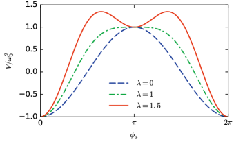
Figure 1: Effective field potential $V$ given in Eq. (5) for different values of $\lambda$. It develops a local minimum at $\phi_{a}=\pm\pi$ for $\lambda>1$. We take $\omega_{0}=1$ here for purposes of illustration.

Here, the potential $V(\phi_{0})$ is plotted in Fig 1, and is given analytically by

$$V(\phi_{a})=-\omega_{0}^{2}\left[\cos(\phi_{a})-\frac{\lambda^{2}}{2}\sin^{2}(\phi_{a})\right],$$ (5)

where we have defined a characteristic frequency $\omega_{0}$ due to the coupling as:

$$\omega_{0}=2\sqrt{\nu g\rho_{0}}/\hbar$$ (6)

and a dimensionless parameter $\lambda$ that parameterizes the depth of Kapitza modulation

$$\lambda^{2}=2\rho_{0}g\delta^{2}/\nu.$$ (7)

To demonstrate the resulting many-body Kapitza pendulum, we solve the time-dependent coupled mean-field Gross-Pitaevskii equations obtained from Eq. (2)

$$i\hbar\partial_{t}\psi_{j} = \left[-\frac{\hbar^{2}}{2m}\nabla^{2}-\mu+g_{jj}|\psi_{j}|^{2}+g_{12}|\psi_{3-j}|^{2}\right]\psi_{j}$$ (8)

$$- [\nu+\delta\hbar\omega\cos(\omega t)]\psi_{3-j},$$

where index $j=1,2$. Oscillations of the relative phase $\phi_{a}$ for two different values of the modulation parameter $\lambda$, for a uniform field, are shown in Fig. 2.

Figure 2: Solutions of Eq. (8) for the relative phase $\phi_{a}$, for different values of the parameter $\lambda^{2}=2\delta^{2}g\rho_{0}/\nu$. The initial state is chosen to be $\psi_{1}=\sqrt{\rho_{0}}$ and $\psi_{2}=\sqrt{\rho_{0}}\exp(i\pi+i0.1)$. For purposes of illustration, we use dimensionless parameters with $\hbar=1$, $g_{12}=0$, $g_{11}=g_{22}=g$, $\mu=g\rho_{0}$+$\nu$, $\rho_{0}=100$, $\nu=0.1g\rho_{0}$, $\omega=50\omega_{0}$. For $\lambda=1.5$, in the red line, the effective potential for the relative phase develops a local minimum at $\phi_{a}=-\pi$, cf Fig. 1. As a result, the phase oscillates around the new local equilibrium value, while at $\lambda=0$ it freely rolls down the hill.

II.2 Effective Hamiltonian

We now consider how to translate this semi-classical result into a quantum dynamical equation, for the general coupling case with arbitrary $g_{ij}$. For such fast oscillations we derive an effective time-independent Hamiltonian ruling the time average dynamics following the approach developed in Ref. Goldman and Dalibard (2014). For a single-harmonic modulation of the form $\hat{H}=\hat{H}_{0}+\hat{H}_{1}\cos(\omega t)$, the effective Hamiltonian reads

$$\hat{H}_{{\rm eff}}=\hat{H}_{0}+\frac{1}{4(\hbar\omega)^{2}}\left[\left[\hat{H}_{1},\hat{H}_{0}\right],\hat{H}_{1}\right]+{\cal O}(1/\omega^{3}).$$ (9)

Here, $\hat{H}_{0}$ is the same as $\hat{H}$ without driving. Using $\hat{H}_{1}=-\delta\hbar\omega\int d{\bf r}\hat{\psi}_{j}^{\dagger}\hat{\psi}_{3-j}$ , the second term in Eq. (9) reads

$$- \frac{(g_{jj}-g_{12})\delta^{2}}{4}\int d{\bf r}\left[\left(\hat{\psi}_{j}^{\dagger}\right)^{2}\left(\hat{\psi}_{3-j}\right)^{2}+\left(\hat{\psi}_{3-j}^{\dagger}\right)^{2}\left(\hat{\psi}_{j}\right)^{2}\right.$$ (10)

$$+ \left.2\hat{\psi}_{j}^{\dagger}\hat{\psi}_{j}^{\dagger}\hat{\psi}_{j}\hat{\psi}_{j}-4\hat{\psi}_{j}^{\dagger}\hat{\psi}_{j}\hat{\psi}_{3-j}^{\dagger}\hat{\psi}_{3-j}\right].$$

The harmonic modulation thus leads to two-particle tunneling processes encapsulated in the first line of Eq. (10) as well as to the modification of the interaction strengths encapsulated in the second line of Eq. (10). To shed light on its nature we ignore density fluctuations and represent the fields as $\psi_{j}\approx\sqrt{\rho_{0}}\exp(i\phi_{j})$, where $\rho_{0}$ and $\phi_{j}$ are the density and the phase of a single component, recalling that we are considering here the symmetric case where both components have equal density, apart from quantum density fluctuations that are neglected at this stage.

Substituting this into Eq. (10) and combining with the single tunneling term $-\nu\int d{\bf r}\hat{\psi}_{j}^{\dagger}\hat{\psi}_{3-j}$ we obtain the mean-field potential energy $U$ felt by the relative phase $\phi_{a}=\phi_{1}-\phi_{2}$

$$U(\phi_{a})\approx-2\nu\sqrt{\rho_{1}\rho_{2}}\left[\cos(\phi_{a})-\frac{\lambda^{2}}{2}\sin^{2}(\phi_{a})\right],$$ (11)

where $\lambda^{2}=2\rho_{0}\delta^{2}\sqrt{(g_{11}-g_{12})(g_{22}-g_{12})}/\nu$. The potential is flattened around $\phi_{a}=\pi$ at $\lambda^{2}\lesssim 1$ and develops a local minimum at $\lambda^{2}>1$. The former is relevant for the studies of the slow-roll of a scalar field, while the later is relevant for the studies of the quantum decay of a scalar field from a metastable minimum. These two fundamental scenarios can be both realized in our system. We have shown that the potential energy $U(\phi_{a})$ in the BEC theory, and the effective scalar field potential $V(\phi_{a})$ are proportional. Next we will use functional integral methods to analyze the phase dynamics.

III Path-Integral representation

In the following section, to facilitate calculations, we will set $g_{12}=0$, $g_{11}=g_{22}=g$, $\rho_{1}=\rho_{2}=\rho_{0}$, so that $\lambda^{2}$ is given in Eq. (7).

We introduce the quantum partition function Atland and Simons (2010)

$${\cal Z}=\int{\cal D}(\psi^{\ast},\psi){\rm e^{-S[\psi^{\ast},\psi]}},$$ (12)

where $S[\psi^{\ast},\psi]=\int d{\bf s}\left[\psi_{j}^{\ast}\partial_{\tau}\psi_{j}+H_{{\rm eff}}(\psi^{\ast},\psi)\right]$ is the action. Here, ${\bf s}=(\tau,{\bf r})$ is a $1+d$ vector, where $\tau=it/\hbar\in[0,\beta]$ is imaginary time. The quantum path integral is taken over all configurations of the complex field $\psi_{j}(\tau,{\bf r})$ with the periodic boundary condition $\psi_{j}({\rm{\bf\beta},{\bf r}})=\psi_{j}(0,{\bf r})$.

We look first for a static solution to identify vacua. This amounts to replacing $\psi_{j}=\psi_{0}={\rm const}$ in the saddle-point approximation $\delta S/\delta\psi_{j}=0$. For $\nu>0$ we obtain the stable $|\psi_{0}|^{2}=(\mu+\nu)/g(1-\delta^{2})$ and unstable $|\psi_{0}|^{2}=(\mu-\nu)/g(1-\delta^{2})$ vacua. These correspond to the two Bose gases being in phase and out-of-phase respectively, although this depends on the sign chosen for the microwave coupling term $\nu$.

Let us introduce new field variables with the definitions $\psi_{j}({\bf s})=\rho_{j}^{1/2}({\bf s})e^{i\phi_{j}({\bf s})}$, where $\rho_{j}({\bf s})=\rho_{0}+\delta\rho_{j}({\bf s})$ and $\rho_{0}=|\psi_{0}|^{2}$. The variables $\delta\rho$ and $\phi$ parametrize the deviation of the Bose fields from a vacuum. Substituting this parametrization of the fields into the action, we obtain

$$\begin{split}S&\approx\int d{\bf s}\left\{i\delta\rho_{j}\partial_{\tau}\phi_{j}+\frac{\hbar^{2}\rho_{0}}{2m}(\nabla\phi_{j})^{2}+\frac{\hbar^{2}}{2g}V(\phi_{a})\right.\\ &+\frac{[2g\rho_{0}(1-\delta^{2})+\nu\cos(\phi_{a})]\delta\rho_{j}^{2}}{4\rho_{0}}+\frac{\hbar^{2}(\nabla\delta\rho_{j})^{2}}{8m\rho_{0}}\\ &-\nu\left[\cos(\phi_{a})-\lambda^{2}\sin^{2}(\phi_{a})\right]\delta\rho_{j}\\ &\left.-\frac{\nu}{4\rho_{0}}\left[\cos(\phi_{a})-2\lambda^{2}\sin^{2}(\phi_{a})-\lambda^{2}\right]\delta\rho_{j}\delta\rho_{3-j}\right\}.\end{split}$$ (13)

Here $\phi_{a}=\phi_{1}-\phi_{2}$ is the relative phase and $V(\phi_{a})$ is the effective potential given in Eq. (5).

The potential $V(\phi_{a})$ develops a local minimum at $\phi_{a}=\pm\pi$ for $\lambda^{2}>1$ (cf. Fig. 1), which corresponds to a false vacuum. Multiple equivalent true vacua occur at the global minima with $\phi_{0}=\pm 0,2\pi,4\pi,\ldots$

Since the action is now quadratic in the density fields, we can perform a Gaussian integration over the density fields. Ignoring gradients acting on the density fields (i.e., the terms $\hbar^{2}(\nabla\delta\rho_{j})^{2}/8m\rho_{0}$) in comparison with the potential cost of these fluctuations (i.e. , the terms $g\delta\rho_{j}^{2}/2$) and introducing relative and total phases, $\phi_{a}=\phi_{1}-\phi_{2}$ and $\phi_{t}=\phi_{1}+\phi_{2}$ respectively, we obtain

$$S\approx\int d{\bf s}\left\{\frac{(\partial_{\tau}\phi_{a})^{2}}{4g[1+\tilde{\nu}\cos(\phi_{a})-\tilde{\nu}\lambda^{2}]}+\frac{\hbar^{2}\rho_{0}}{4m}(\nabla\phi_{a})^{2}+\frac{\hbar^{2}}{2g}V^{\prime}(\phi_{a})\right.$$

$$\left.+\frac{1}{4g}(\partial_{\tau}\phi_{t})^{2}+\frac{\hbar^{2}\rho_{0}}{4m}(\nabla\phi_{t})^{2}+\frac{\nu}{g}i\partial_{\tau}\phi_{t}F[\phi_{a}]\right\}.$$ (14)

Here we have denoted

$$F[\phi_{a}]=\cos(\phi_{a})-\lambda^{2}\sin^{2}(\phi_{a}),$$ (15)

and introduced an effective potential for the relative phase modified by the presence of the environment as

$$V^{\prime}(\phi_{a})=V(\phi_{a})+2\frac{\nu^{2}}{\hbar^{2}}\left[\cos(\phi_{a})-\lambda^{2}\sin^{2}(\phi_{a})\right]^{2}.$$ (16)

The action (14) contains two fields, the relative and the total phases, coupled by the last term in Eq. (14). The total phase field is characterized by the speed of sound $c=\sqrt{g\rho_{0}/m}$. In contrast to this, the relative phase is characterized by a modified speed of sound, which in the semiclassical limit $\lambda\gg 1$ (see below) is given by $c_{a}=\sqrt{g\rho_{0}(1-\tilde{\nu}\lambda^{2})/m}$, where $\tilde{\nu}=\nu/(g\rho_{0})$.

Apart from some corrections from the environmental degrees of freedom, which are higher order effects that are omitted here for simplicity, the effective action for the relative phase now reads

$$S_{a}(\phi_{a})\approx\frac{\hbar^{2}}{2g}\int d{\bf s}\left[\frac{1}{2\hbar^{2}}(\partial_{\tau}\phi_{a})^{2}+\frac{c_{a}^{2}}{2}(\nabla\phi_{a})^{2}+V^{\prime}(\phi_{a})\right].$$ (17)

This action corresponds to the equation of motion given in Eq. (1) with the replacement $\phi\rightarrow\phi_{a}$ and $V\rightarrow V^{\prime}(\phi)$ given in Eq. (16). We have thus arrived at a quantum field model similar to Coleman’s original model for the false vacuum decay.

The action in Eq. (14) is quadratic in the total phase fields $\phi_{t}$ and we can again perform a Gaussian integration, this time over the total phase fields. This yields our final result, that includes the effect of the environmental density fluctuations omitted in Eq. (17):

$$\begin{split}S(\phi_{a})=&\frac{\hbar^{2}}{2g}\int d{\bf s}\left[\frac{1}{2\hbar^{2}}(\partial_{\tau}\phi_{a})^{2}+\frac{c_{a}^{2}}{2}(\nabla\phi_{a})^{2}+V^{\prime}(\phi_{a})\right]\\ &+\frac{\nu^{2}}{g}\int d{\bf s}\int d{\bf s}^{\prime}F[\phi_{a}({\bf s})]F[\phi_{a}({\bf s}^{\prime})]{\cal G}({\bf s}-{\bf s}^{\prime}),\end{split}$$ (18)

where

$$\begin{split}{\cal G}(\tau,x)&=\frac{1}{\beta L^{d}}\sum_{\omega_{n},{\bf k}}e^{-i(\omega_{n}\tau+kx)}\frac{\omega_{n}^{2}}{\omega_{n}^{2}+(c\hbar k)^{2}}\end{split}$$ (19)

is a non-local kernel responsible for long-range correlations in the relative phase sector induced by the environmental degrees of freedom. For example, at zero temperature and one spatial dimension it can be evaluated as

$${\cal G}(\tau,x)=\frac{\hbar c}{2\pi}\frac{x^{2}-(\hbar c)^{2}\tau^{2}}{[x^{2}+(\hbar c)^{2}\tau^{2}]^{2}}.$$ (20)

In two and three dimensions expressions for the corresponding higher dimensional kernel ${\cal G}(\tau,{\bf r})$ are more involved, and will not be treated here. The effect of the additional non-local term (the second line in Eq. (18)) on the dynamics of the relative phase are explored in the next section.

IV Tunneling rate

To quantify the tunneling process, we calculate the probability that the system has not yet decayed at time $t$. At long time scales it should behave as ${\cal F}=\exp(-\Gamma t)$ Takagi (2006), where $\Gamma$ is the decay rate from the false vacuum. In the weak tunneling limit it can be written in the form $\Gamma=A\exp(-B)$. The coefficients $A\propto B^{2}$ and $B$ were calculated in the context of the false vacuum decay using the instanton technique in Refs. Coleman (1977); Callan and Coleman (1977), in some limiting cases. The decay rate of phase slips in the O(2) quantum rotor model was calculated in Ref. Danshita and Polkovnikov (2012).

Here we use the instanton technique to estimate the coefficient $B$ and the form of the bubbles. This approach is not strictly valid for shallow potentials with $\lambda\rightarrow 1$, but it should provide reasonable estimates provided that $\lambda-1$ is not too small. Calculating the coefficitient $B$ allows to extract the decay rate $\Gamma$ to a level of exponential accuracy. This estimate for $\Gamma$ is independent on the initial state. Quantum corrections are hidden in the coefficient $A$. However, the calculation of the coefficient $A$ is a rather complicated problem in quantum field theory Callan and Coleman (1977) and will be omitted here. We focus in particular on certain scaling relations which appear universal. These will be verified in detailed numerical quantum dynamical simulations in the next section.

In order to calculate $B$ we need to find first a bounce solution of the equation of motion corresponding to the imaginary-time action (17). We treat the induced additional term in Eq. (18) as perturbation to be included later. Varying the action (17) with respect to the field $\phi_{a}({\bf s})$ and setting $R=\sqrt{{\bf r}^{2}+(c_{a}\hbar\tau)^{2}}$, we find a solution $\phi_{B}$ to the equation of motion, given by

$$\left(\partial_{R}^{2}+\frac{d}{R}\partial_{R}\right)\phi_{B}=c_{a}^{-2}\partial_{\phi_{B}}V^{\prime}(\phi_{B}),$$ (21)

which must be solved subject to the boundary condition $\phi_{B}(R=\infty)=\pi$ and $\partial_{R}\phi_{B}(R=0)=0$ Coleman (1977).

Here, $d$ is the total number of space dimensions, since this equation is also valid in higher dimensions. Eq. (21) describes a fictitious particle with coordinate $\phi_{B}$. It is released at rest at some position $\phi_{B}(R=0)$ and approaches $\phi_{B}(R=\infty)=\pi$ at long times. For not too small $\lambda-1$, we may assume $\phi_{B}(R=0)=0$ or $\phi_{B}(R=0)=2\pi$ and adopt the thin-wall approximation by ignoring the friction term in Eq. (21).

The bounce solution can now be easily found from Eq. (21)

$$\phi_{B}(R)\approx 2\arctan\left(\exp\left[\frac{\lambda\omega_{0}(R-R_{B})}{c_{a}}\right]\right),$$ (22)

where $R_{B}$ is the radius of the bubble. Inside the bubble ($R\ll R_{B}$) we get the true vacuum solution of $\phi_{B}(R)=0$ or $2\pi$, while outside the bubble ($R\gg R_{B}$) we get $\phi_{B}(R)=\pi$ as expected.

The coefficient $B$ can now be calculated as $B=S_{a}[\phi_{B}]$, or more explicitly

$$B=\Omega_{d+1}\frac{\hbar c_{a}}{2g}\int_{0}^{\infty}dRR^{d}\left[\frac{1}{2}(\partial_{R}\phi_{B})^{2}+\frac{1}{c_{a}^{2}}V^{\prime}(\phi_{B})\right],$$ (23)

where $\Omega_{d+1}=2\pi^{(d+1)/2}/\Gamma[(d+1)/2]$ is the solid angle in $d+1$ total space-time dimensions. Using the bounce solution (22) we get the semiclassical estimate $B=\Omega_{d+1}R_{B}^{d}\lambda\hbar\omega_{0}\left(1-R_{B}\omega_{0}/2\lambda c_{a}\right)/g$.

Minimizing $B$ with respect to $R_{B}$ we obtain the radius of the nucleated bubble $R_{B}=2d\lambda c_{a}/[\omega_{0}(d+1)]$ and

$$B=\Omega_{d+1}\frac{\lambda\hbar\omega_{0}}{dg}\left[\frac{2d\lambda c_{a}}{\omega_{0}(d+1)}\right]^{d}.$$ (24)

Once a bubble with radius $R_{B}$ and rate $\Gamma\propto\exp(-B)$ is nucleated, it expands with the speed $c_{a}$, which is slightly smaller than the speed of sound.

In one dimension we get $B=2\pi\lambda^{2}\hbar c_{a}/g\propto\lambda^{2}\rho_{0}\xi$, where $\xi=\hbar/\sqrt{2mg\rho_{0}}$ is the healing length. We now substitute $\phi_{B}(R)$ into the second line of Eq. (18). After a proper rescaling of variables under the integral this leads to the correction $\Delta B\approx\lambda^{4}\tilde{\nu}^{2}\rho_{0}\xi$. Combining with the semiclassical estimate we arrive at

$$B_{1D}=\left(\beta(\lambda)+\gamma(\lambda)\tilde{\nu}^{2}\right)\rho_{0}\xi.$$ (25)

Here $\beta(\lambda)$ and $\gamma(\lambda)$ are complicated expressions in general, and cannot be easily obtained precisely outside of the thin-wall limit of Coleman.

We note that the theory generally predicts a quadratic dependence on $\tilde{\nu}^{2}$, which we show does agree with quantitative numerical simulations in the next section. At large values of $\lambda$ the semiclassical analysis in the thin-wall limit yields $\beta(\lambda)\propto\lambda^{2}$and $\gamma(\lambda)\propto\lambda^{4}$. It also follows that the effect of the non-local correlations on the quantum tunneling process in one dimension is small in the sine-Gordon regime where $\tilde{\nu}\ll 1$.

V Numerical Analysis

The path integral calculations given above are indicative of the potential for simulating the decay of a relativistic quantum field metastable vacuum using an ultra-cold atomic BEC.

Yet how practical is this, really? How accurate are the approximations used? Most crucially, how long will tunneling take? This last question is an important one, because current laboratory BEC experiments are limited in time duration by trap losses. These in turn depend on many issues, ranging from the vacuum quality to the size of nonlinear loss effects due to collisions. Depending on the isotope used and the density, the lifetime typically varies between millisecond to seconds, in current experiments.

Neither the tunneling prefactor $A$ nor the exponent $B$ is easily calculable for our system. Even B is known only in the simplest of cases, so it is not possible to analytically obtain an estimated tunneling time. We instead resort to numerical simulations of the full quantum field dynamics, which has a number of advantages. The full dynamics of using BECs with modulated coupling is easily included, and one can also include laboratory losses. Most significantly, one is not restricted to the slow tunneling, deep well regime as in Coleman’s original work. This is fortunate, since the slow tunneling regime is neither suited to experiments, nor well matched to currently proposed cosmological models.

The truncated Wigner approximation (TWA), where a quantum state is represented by a phase space distribution of stochastic trajectories following the Gross-Pitaevskii equation Drummond and Hardman (1993); Steel et al. (1998) together with dissipative noise terms, enables one to capture many quantum features of the system. This method gives the first quantum correction to the Gross-Pitaevskii equation, in an expansion in $M/N$, where $M$ is the number of modes and $N$ is the total number of bosons. It is known to correctly predict quantum fluctuation dynamics in a number of quantitative experiments at the quantum noise level Drummond and Chaturvedi (2016). We use this approach to perform stochastic numerical simulations on the full BEC model in order to investigate true vacuum nucleation numerically. The TWA generally needs to be checked with more precise methods Deuar and Drummond (2006). From previous work we expect it to be able to generate tunneling times that are accurate enough to give estimates of useful experimental parameter values.

This approach was originally used to predict quantum squeezing dynamics in photonic quantum solitons Carter et al. (1987); Drummond et al. (1993), which have a combination of quantum field propagation and dissipative coupling to phonon reservoirs. The truncation approximation was justified by comparisons to exact positive-P quantum dynamical theory Drummond and Hardman (1993), and gave excellent quantitative, first principles agreement with high-precision experimental measurements Corney et al. (2006). Succesful comparisons with BEC interferometry in three dimensions have been made, showing that this approach is applicable to bosonic atoms. Tunneling in shallow potentials for related parametric systems Drummond and Kinsler (1989) has been treated, giving agreement with exact methods. However, the truncated Wigner method can become inaccurate when treating deeper wells, or systems where scattering into unoccupied vacuum modes in three dimensions is a dominant feature Deuar and Drummond (2007). This is a possible limitation when treating tunneling in higher space dimensions, since the true vacuum spatial modes will not be highly occupied initially.

We simulate the false vacuum decay in one spatial dimension. BEC is impossible in low-dimensional homogenous systems, but it should occur when atoms are trapped because the confining potential modifies the density of states Bagnato and Kleppner (1991). It can be realized in low-dimensional optical and magnetic traps in which the energy-level spacing exceeds interparticle interaction and temperature Görlitz et al. (2001), and we give a quantitative estimate of the relevant coherence length in the last section. The initial quantum state is assumed to be a highly occupied Bose-Einstein condensate in a coherent state. The coherent state distribution for the corresponding Wigner phase-space distribution is a Gaussian in phase space, and the vacuum modes have a corresponding initial variance of $n=1/2$. Our initial state construction for the Wigner representation then proceeds by simply including vacuum noise for each mode to the coherent state. The primary physical effect of the initial noise is to allow spontaneous scattering processes that are disallowed in pure Gross-Pitaevskii theory. Additional noise is required when there is damping, in order to correctly model the fluctuation-dissipation properties of a quantum phase-space representation of this type.

Typical results are presented as single trajectories in the plots included here, for illustrative purposes. Given that the universe is, in current cosmology, a single quantum wavefunction, it is a subtle question to understand how these trajectories can be compared to cosmological events. The use of a Wigner representation to generate such trajectories is motivated by the fact that the marginal probabilities of the Wigner distribution are true, classical-like probabilities Hillery et al. (1984). This depends on the observations Lewis-Swan et al. (2016), and is surely only a first step towards understanding this hypothesis.

As the predicted behaviour is stochastic, the computed tunneling rates to be compared with a future experiment require and utilize a full quantum ensemble average. More fundamentally, our philosophy is that one should understand the proposed experiment as a quantum computer for this unsolved dynamical quantum field problem. Given that our computer simulations embody a truncation approximation, they should not be regarded as definitive. An indicator of the breakdown of the TWA would be tunneling rates that are faster than anticipated.

The chief limitation of this approach is that it neglects one of the likely features of an experiment, which is that the initial state will be generated dynamically by Rabi rotating a finite temperature equilibrium ensemble, which could alter the tunneling times. We do not treat this in the present study. However, the use of an initial coherent state does correctly model the correlations induced by the Rabi rotation process. Methods that treat finite temperature effects are known Ruostekoski and Isella (2005), and will be carried out in another publication. While it is certainly possible that the precise initial quantum state may have an effect on tunneling, the best candidate quantum state for early universe modeling is not well understood. One longer term goal of this research is to determine whether cosmological data can throw any light on this question, which will require further modeling and experiments with different initial quantum states.

V.1 Symmetric BEC experiment

The first case we consider is the idealized case treated analytically in the previous section, with equal intra-state scattering lengths, and zero inter-state scattering lengths. The stationary solution of the two independent condensates at the classical level is found by solving the Gross-Pitaevskii equation in imaginary time, without any linear coupling between the two species. The initial conditions are $\psi_{j}=\sqrt{\rho_{0}}\exp[i(j-1)\pi]$, such that the number densities $\rho_{j}=|\psi_{j}|^{2}$ are the same and the relative phase is $\pi$. Next, quantum noise corresponding to a coherent state is added to this state as $\psi(x)\rightarrow\psi(x)+\sum_{i=1}^{M}\alpha_{i}\exp(ik_{i}x)/\sqrt{L}$. Here $\alpha_{i}$ are complex Gaussian variables with $\overline{\alpha_{i}^{\ast}\alpha_{k}}=\delta_{ik}/2$, thus sampling vacuum or coherent state fluctuations. The number of modes $M$ is chosen to represent the physical system, while being much smaller than the total number of atoms $N$, so that $M/N\ll 1$, as required for the truncated Wigner method.

We propagate this state in real time by solving the time-dependent coupled mean-field equations (8). In the absence of damping and noise, the corresponding equations for the Wigner representation are:

$$i\hbar\frac{d\Psi_{j}}{dt}=-\frac{\hbar^{2}}{2m}\frac{\partial^{2}\Psi_{j}}{\partial x^{2}}+g\Psi_{j}\left(|\Psi_{j}|^{2}-\delta_{M}-\frac{\mu}{g}\right)-\nu_{t}\Psi_{3-j}.$$ (26)

where for the plane wave basis $\delta_{M}=M/L$. For our numerical calculations we use dimensionless variables. These are defined by scaling time in terms of the characteristic frequency $\omega_{0}=2\sqrt{\nu g\rho_{0}}/\hbar$, and scaling space by combining this with the speed of sound $c=\sqrt{g\rho_{0}/m}$. The resulting units of time are $\tilde{t}=t\omega_{0}$, length $\tilde{x}=x/x_{0}=x\omega_{0}/c$ and energy $\tilde{\nu}=\nu/g\rho_{0}$.

The equations of motion in the new units become

$$i\frac{d\tilde{\Psi}_{j}}{d\tilde{t}}=\left[-\sqrt{\tilde{\nu}}\frac{\partial^{2}}{\partial\tilde{x}^{2}}+\frac{|\tilde{\Psi}_{j}|^{2}-\tilde{\delta}_{M}}{2\sqrt{\tilde{\nu}}\tilde{\rho}_{0}}+\frac{\tilde{\nu}-1}{2\sqrt{\tilde{\nu}}}\right]\tilde{\Psi}_{j}$$

$$-\frac{\sqrt{\tilde{\nu}}}{2}\left[1+\sqrt{2}\lambda\tilde{\omega}\cos(\tilde{\omega}\tilde{t})\right]\tilde{\Psi},$$ (27)

where $\lambda=\delta\sqrt{2}/\sqrt{\tilde{\nu}}$, $\tilde{\rho}_{0}=\rho_{0}x_{0}$ and $\tilde{\delta}_{M}=Mx_{0}/L$.

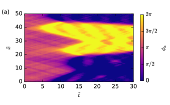
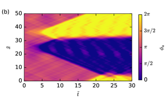
Figure 3: Decay of the false vacuum in 1D. (a) A single-trajectory simulation of the false vacuum decay in 1D with $N_{\mathrm{grid}}=256$ and dimensionless parameters $\lambda=1.3$, $\tilde{\omega}=50$, $\tilde{\nu}=2\times 10^{-3}$, $\tilde{L}=50$, $\tilde{\rho}_{0}=1000$, $a_{11}=3a_{0}$, $a_{22}=20a_{0}$, $a_{12}=0$ (corresponding to a two-component ⁷Li condensate near $640\,\mathrm{G}$ resonance in a ring trap with $N=5\times 10^{4}$, trap circumference $L=121.7\,\mathrm{\mu m}$, transverse frequency $\omega_{\perp}=2\pi\times 61\,\mathrm{kHz}$, observation time $T=1.75\,\mathrm{ms}$, oscillator amplitude $\nu/\hbar=2\pi\times 61\,\mathrm{Hz}$, frequency $\omega=2\pi\times 136.4\,\mathrm{kHz}$ and modulation $\delta=0.041$). The initial component population ratio $N_{1}/N_{2}\approx 0.872/0.128$ (obtained by solving Eq. (35) numerically for $\theta$, with $N_{1}/N_{2}\equiv\cot^{2}\theta$). (b) Same parameters as in the previous panel, except the scattering lengths have been set to $a_{11}^{\prime}=a_{22}^{\prime}=\left(a_{11}+a_{22}\right)/2$, to give the symmetric case.

The results of typical simulations in one dimension are shown in Fig. 3. The single trajectory dynamics features the creation of four bubbles in the asymmetric case, treated in detail in the next section, or two bubbles in the symmetric case.

We note here a highly characteristic feature of this type of tunneling, which is the creation of topologically distinct vacua depending on whether the tunneling occurred with a positive or negative phase change. Even though these vacua are locally indistinguishable, they are globally distinct. In the absence of large density changes, they cannot combine with each other, as they are necessarily separated by a high energy region of false vacuum. Collisions of bubbles result either in the creation of localized oscillating structures known as oscillons Amin et al. (2012), or domain walls if the colliding bubbles belong to topologically distinct vacua. Such topologically distinct vacua, if they occurred in the real universe, would presumably have to occur at cosmologically large separations.

In our numerical simulations of tunneling, we fix $\tilde{\rho}_{0}=200$. Therefore, recalling that $\tilde{\nu}=\nu/g\rho_{0}$, we can express the density dependent factors in Eq. (25) in terms of the scaled coupling constant $\tilde{\nu}$ as:

$$\rho_{0}\xi=\tilde{\rho}_{0}\xi/x_{0}=\tilde{\rho}_{0}\omega_{0}\xi/c=\tilde{\rho}_{0}\sqrt{2\tilde{\nu}}\,.$$ (28)

Substituting this expression for $\rho_{0}\xi$ into Eq. (25) we obtain an expected scaling law at fixed $\tilde{\rho}_{0}$ where the exponents increase by $1/2$, so that:

$$B_{1D}(\lambda,\tilde{\nu})=\tilde{\beta}(\lambda)\tilde{\nu}^{1/2}+\tilde{\gamma}(\lambda)\tilde{\nu}^{5/2},$$ (29)

where $\tilde{\beta}=\sqrt{2}\tilde{\rho}_{0}\beta$ and $\tilde{\gamma}=\sqrt{2}\tilde{\rho}_{0}\gamma$.

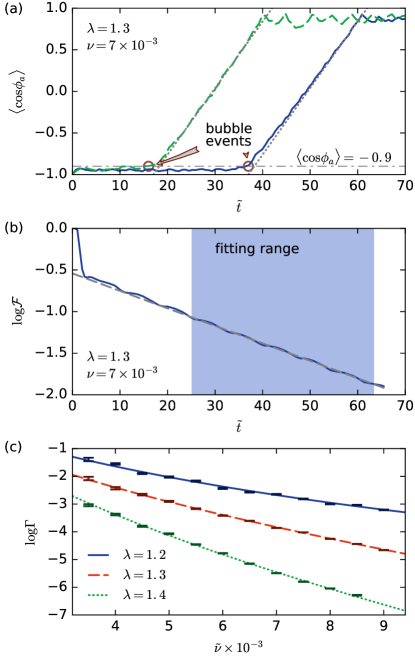
Figure 4: (a) Average relative phase $\langle\cos\phi_{a}\rangle$ in two separate single-trajectory simulations. A bubble is detected at $\tilde{t}=16$ and $\tilde{t}=37$. (b) Logarithmic plot of the survival probability $\mathcal{F}$ estimated using $16384$ TWA trajectories. The standard error in the mean is smaller than the line thickness and, therefore, not shown in the graph. The long time scale part of the plot (marked with the blue background) is fitted with a linear dependence (that is, ${\cal F}=\exp(-\Gamma\tilde{t})$), the slope of which gives the negated tunneling rate $-\Gamma$. (c) Dependence of the tunneling rate $\Gamma$ on the coupling $\tilde{\nu}$ for different values of $\lambda$. The errorbars show the combination of two sources of errors: the standard error in the mean of $\mathcal{F}$ and the estimated error of the linear fitting of $\log\mathcal{F}$. We fitted the data with $\log(\Gamma)=\tilde{\alpha}+\tilde{\beta}\tilde{\nu}^{1/2}+\tilde{\gamma}\tilde{\nu}^{5/2}$, where $\{\tilde{\alpha},\tilde{\beta},\tilde{\gamma}\}=\{1.72(8),-1.69(3),6.2(4)\times 10^{-4}\}$ for $\lambda=1.2$, $\{1.9(2),-2.14(9),-4(3)\times 10^{-4}\}$ for $\lambda=1.3$, $\{\tilde{\alpha},\tilde{\beta},\tilde{\gamma}\}=\{2.9(4),-3.1(2),-6(11)\times 10^{-4}\}$ for $\lambda=1.4$.

Varying $\tilde{\nu}$ and keeping $\lambda$ fixed allows us to study the quantum dynamics of the scalar field. Our TWA approach is expected to yield accurate predictions for the relatively shallow effective potentials necessary for tunneling over laboratory time-scales Drummond and Kinsler (1989). In Fig. 4 we present the scaling of the tunneling rate of the bubbles as a function of $\tilde{\nu}$ for different values of $\lambda$. The fitting procedure is as follows.

In each trajectory we define the appearance of a bubble as the average relative phase $\langle\cos\phi_{a}\rangle\equiv\frac{1}{\tilde{L}}\int_{0}^{\tilde{L}}\cos\phi_{a}(\tilde{x})d\tilde{x}$ first exceeding the (empyrically chosen) threshold of $0.9$, as illustrated in Fig. 4(a).

From the set of times $\tilde{t}_{j}^{\mathrm{bubble}}$ obtained this way in each of the $N_{\mathrm{tr}}$ TWA trajectories we approximate the decay probability as $\mathcal{F}_{\mathrm{decay}}\left(\tilde{t}\right)\equiv\int_{0}^{t}{\cal P}(\tilde{t}^{\prime})d\tilde{t}^{\prime}\approx\left|\left\{j,\,\tilde{t}_{j}^{\mathrm{bubble}}<\tilde{t}\right\}\right|$. At each point of time we can consider the set of decayed/non-decayed trajectories to be a sample from a binomial distribution and estimate the standard error of the mean as $E_{\mathcal{F}}\approx\sigma\left(\mathcal{F}\right)/\sqrt{N_{\mathrm{tr}}}=\mathcal{F}_{\mathrm{decay}}\left(1-\mathcal{F}_{\mathrm{decay}}\right)\sqrt{N_{\mathrm{tr}}}$. The “survival” probability defined as ${\cal F}\left(\tilde{t}\right)=1-\mathcal{F}_{\mathrm{decay}}$ for one of the values of $\lambda$ and $\tilde{\nu}$ is plotted in Fig. 4(b). The propagated error of $\log\mathcal{F}$, $E_{\mathcal{F}}/\mathcal{F_{\mathrm{decay}}}$, is smaller than the thickness of the line and is not shown on the plot.

The long time scale region is defined as the part of the evolution between the values of the relative population difference $P_{z}=0$ and $P_{z}=-0.5$. The relative population difference is calculated as $P_{z}=\left(N_{2}-N_{1}\right)/\left(N_{1}+N_{2}\right)$, where $N_{1}$ and $N_{2}$ are the component populations after a $\pi/2$ Rabi rotation. The “survival” probability in this region is fitted with an exponential, shown as the dashed grey line in Fig. 4(b) using weighted least squares (WLS), with weights being the errors of the mean from the previous step. This resultes in the value of the slope of the log plot $-\Gamma$, along with the associated error, for each pair of $\tilde{\nu},\lambda$. These points with errorbars are shown in Fig. 4(c).

Since $\Gamma=A\exp(-B)$, where $B$ is given in Eq. (29), we fit the curves with $\log(\Gamma)=\tilde{\alpha}+\tilde{\beta}\tilde{\nu}^{1/2}+\tilde{\gamma}\tilde{\nu}^{5/2}$, where $\tilde{\alpha}=\log(A)$. We were only able to fit the value of $\tilde{\gamma}$ accurately for $\lambda=1.2$, while for higher values of $\lambda$ the estimated error is comparable to the fitted value of the coefficient. Overall, the observed behavior provides strong evidence of a quantum tunneling process leading to bubble nucleation, with a scaling dependence on $\tilde{\nu}$ that agrees with the path integral result, Eq. (25).

V.2 Non-zero inter-component interaction

While the previous analysis treated the symmetric case, not all atomic species have this type of Hamiltonian. We therefore turn to the more general case typical, for example, of the broad Feshbach resonance known to occur in ⁷Li.

The most general equation of motion for TWA approach corresponding to the Hamiltonian (2) reads:

$$i\hbar\frac{d\Psi_{j}}{dt}=-\frac{\hbar^{2}}{2m}\frac{\partial^{2}\Psi_{j}}{\partial x^{2}}+\\ \sum_{k=1}^{2}g_{jk}\left(|\Psi_{k}|^{2}-\frac{\delta_{jk}+1}{2}\delta_{M}-\mu\right)\Psi_{j}-\nu_{t}\Psi_{3-j}.$$ (30)

This equation is similar to Eq. (26). We now allow the inter-component interaction strength $g_{12}\neq 0$ as well as the possibility $g_{11}\neq g_{22}$.

Similarly to the derivation of Eq. (27) we introduce units of time $\tilde{t}=t\omega_{0}$ and length $\tilde{x}=x/x_{0}=x\omega_{0}/c$, where now $c=\sqrt{\bar{g}\rho_{0}/m}$, $\bar{g}=(g_{11}+g_{22})/2+g_{12}$, and $\omega_{0}=2\sqrt{\nu\bar{g}\rho_{0}}/\hbar$. The chemical potential is taken so that $\mu=\bar{g}\rho_{0}+\nu$. Denoting $\tilde{\nu}=\nu/\bar{g}\rho_{0}$, $\tilde{g}_{jk}=g_{jk}/\bar{g}$, and $\lambda=\delta\hbar\omega_{0}/\sqrt{2}\nu$, we arrive at

$$i\frac{d\tilde{\Psi}_{j}}{d\tilde{t}}=\left[-\sqrt{\tilde{\nu}}\frac{\partial^{2}}{\partial\tilde{x}^{2}}+\sum_{k=1}^{2}\frac{\tilde{g}_{jk}}{2\sqrt{\tilde{\nu}}\tilde{\rho}_{0}}\left(|\tilde{\Psi}_{k}|^{2}-\frac{\delta_{jk}+1}{2}\tilde{\delta}_{M}\right)\right]\tilde{\Psi}_{j}$$

$$+\frac{\tilde{\nu}-1}{2\sqrt{\tilde{\nu}}}\tilde{\Psi}_{j}-\frac{\sqrt{\tilde{\nu}}}{2}\left[1+\sqrt{2}\lambda\tilde{\omega}\cos(\tilde{\omega}\tilde{t})\right]\tilde{\Psi}_{3-j},$$ (31)

where $\tilde{\rho}_{0}=\rho_{0}x_{0}$ and $\tilde{\delta}_{M}=Mx_{0}/L$.

First of all, we need to find appropriate initial conditions for simulating Eq. (31). The dynamics of the classical fields $\psi_{j}$ is governed by the potential function:

$${\cal H}=\frac{g_{jk}}{2}|\psi_{k}|^{2}|\psi_{j}|^{2}-\nu\psi_{j}^{\ast}\psi_{3-j},$$ (32)

where summation over spin indices $j$ and $k$ is assumed as in Eq. (2).

We parameterize the field $\psi_{1}$ and $\psi_{2}$ as

$$\psi_{1} = u\exp\left[i\left(\phi_{s}+\phi_{a}\right)/2\right]\cos\theta,$$

$$\psi_{2} = u\exp\left[i\left(\phi_{s}-\phi_{a}\right)/2\right]\sin\theta.$$ (33)

and adopt the dimensional units introduced above to get:

$${\cal H}\equiv u^{4}g\tilde{{\cal H}}=\\ u^{4}g\left(-\tilde{\nu}\cos\phi_{a}\sin 2\theta+\frac{\tilde{g}_{s}}{2}+\frac{\tilde{g}_{sa}}{2}\cos^{2}2\theta+\tilde{g}_{a}\cos 2\theta\right).$$ (34)

The initial conditions are found from the two saddle-point equations $\partial\tilde{{\cal H}}/\partial\phi_{a}=0$ and $\partial\tilde{{\cal H}}/\partial\theta=0$, or

$$\tilde{\nu}\sin\phi_{a}\sin 2\theta=0,$$ (35)

$$-2\tilde{\nu}\cos\phi_{a}\cos 2\theta-2\tilde{g}_{sa}\sin 2\theta\cos 2\theta-2\tilde{g}_{a}\sin 2\theta=0.$$

Among the various solutions to the above equations, we are interested in solutions satisfying $\partial^{2}\tilde{V}/\partial\theta^{2}>0$ and

$$\frac{\partial^{2}\tilde{{\cal H}}}{\partial\phi_{a}^{2}}\frac{\partial^{2}\tilde{{\cal H}}}{\partial\theta^{2}}-\left(\frac{\partial^{2}\tilde{{\cal H}}}{\partial\phi_{a}\partial\theta}\right)^{2}<0.$$ (36)

In the symmetric case $g_{11}=g_{22}$, we obtain $\psi_{j}=\sqrt{\rho_{0}}\exp[i(j-1)\pi]$. In the more general case $g_{11}\neq g_{22}$ Eqs. (35) and Eq. (36) are solved numerically. Typical results of these numerical simulations are shown in Fig. 3. Although the change in symmetry modifies the dynamics, we see that the essential feature of false vacuum decay into a true vacuum is still found.

V.3 Energy calculations

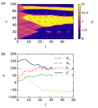
Figure 5: Evolution of relative phase (a) and its energy (b) for $\lambda=1.1$, $\tilde{\omega}=50$, $\tilde{\nu}=0.01$, $\tilde{\rho}_{0}=200$, $a_{11}=a_{22}$, $a_{12}=0$ with $256$ spatial grid points and $160000$ time steps.

We now consider the fate of the potential energy liberated during vacuum tunneling. In a pure quantum vacuum tunneling theory, all forms of energy are conserved. Here, it is possible that energy can be converted from relative phase energy to relative density energy, since density fluctuations act as a reservoir. This is similar to the way that gravitational degrees of freedom can modify the quantum field dynamics in inflationary universe theories.

The energy was calculated as follows. The total energy of the phase Hamiltonian is:

$$E=V+K_{x}+K_{t},$$ (37)

where we divide up the energy into a phase potential energy part, and contributions from the space and time ‘kinetic’ energy terms, which correspond to the energy available for free particle creation in a cosmological interpretation:

$$V=-\int_{0}^{L}\left(\cos\phi_{a}-\frac{\lambda^{2}}{2}\sin^{2}\phi_{a}\right)d\tilde{x},$$

$$K_{x}=\int_{0}^{L}\frac{1}{2}\left(\frac{d\phi_{a}}{d\tilde{x}}\right)^{2}d\tilde{x},$$

$$K_{t}=\int_{0}^{L}\frac{1}{2}\left(\frac{d\phi_{a}}{d\tilde{t}}\right)^{2}d\tilde{x}\,.$$ (38)

Fig. 5 shows the results of energy calculations for one TWA trajectory. The energy was measured at $2000$ time points, then each $20$ values were averaged producing $100$ points in total, which were plotted. Therefore the averaging time window consisted of $\tilde{t}_{\max}/\left(2000/20\right)/\left(2\pi/\tilde{\omega}\right)\approx 4$ periods of the oscillation of the driving field.

As can be seen from the figure there is strong evidence for conversion of energy from potential to ‘kinetic’ energy after a tunneling event has occurred. This implies that, at least at short times after tunneling has occurred, the phase-sector energy is largely conserved. At longer times, the total energy stored in the relative phase sector decreases gradually. We interpret this as transformation of phase-sector energy to relative density fluctuation energy — a behaviour not found in the original Coleman model. This is in accordance with the path integral results and numerical results presented in Fig. 4. The decrease of the tunneling rate found in these studies is associated with a damping mechanism in the system, which is clearly seen in the energy graphs.

VI Experimental proposal

The experimental implementation of false vacuum decay in a two-component Bose-Einstein condensate requires the use of two atomic states with specific scattering properties: (i) the inter-state scattering length should be close to zero, and (ii) both states should have positive scattering lengths so that our parameter $\lambda$ has a real value (section II A). It is also favorable for clear observation of this effect to use the states with nearly identical values of intra-state scattering lengths, in order to avoid the excitation of collective oscillations and the dynamical evolution of the order parameter Egorov et al. (2011).

Two pairs of Zeeman states in ${}^{41}{\rm K}$ have these requisite scattering properties, and can be used to test for the symmetric case of the false vacuum decay. States $|1\rangle=|F=1,m_{F}=1\rangle$ and $|2\rangle=|F=1,m_{F}=0\rangle$ are predicted Lysebo and Veseth (2010) to have an inter-state Feshbach resonance with a zero-crossing of the cross-coupling term $a_{12}$ at $675.25\,\mathrm{G}$, and a resonance width of $0.156\,\mathrm{G}$. The two intra-state scattering lengths have a similar value: $a_{11}=59.5a_{0}$ and $a_{22}=60.5a_{0}$, where $a_{0}$ is the Bohr radius. States $|1\rangle$ and $|2\rangle$ are separated by $61.93\,\mathrm{MHz}$ at this magnetic field, and will be coupled by the amplitude-modulated radio-frequency field via a magnetic dipole transition. The remaining state $|F=1,m_{F}=-1\rangle$ in this hyperfine manifold is far detuned, with a transition frequency of $66.1\,\mathrm{MHz}$, and will not participate in the resonant coupling of the $|1\rangle-|2\rangle$ transition. Another pair of suitable states consists of states $|1\rangle=|F=1,m_{F}=-1\rangle$ and $|2\rangle=|F=1,m_{F}=0\rangle$, which are also predicted Lysebo and Veseth (2010) to have an inter-state Feshbach resonance with a zero-crossing of the cross-coupling at $717.6\,\mathrm{G}$. In this case, the resonance width is $0.118\,\mathrm{G}$, with $a_{11}=61a_{0}$ and $a_{22}=59a_{0}$.

The asymmetric case of the false vacuum decay can be studied with two Zeeman states $|1\rangle=|F=1,m_{F}=0\rangle$, and $|2\rangle=|F=1,m_{F}=1\rangle$ in a ⁷Li condensate. These two states have zero-crossing of the inter-state scattering length $a_{12}$ at 640 G and positive values of scattering lengths $a_{11}=3a_{0}$ and $a_{22}=20a_{0}$ Hulet , as in the conditions of Fig. 3(a). The ⁷Li condensate can be readily prepared in one of the two Zeeman states, and the inter-state coupling can be driven by radiofrequency radiation in a similar way as with ⁴¹K atoms.

We can estimate the phase coherence length for the experimental parameters quoted in the caption of Fig. 3(a). The dimensionless coupling parameter is

$$\gamma=\frac{m\bar{g}}{\hbar^{2}\rho_{0}}=1.25\times 10^{-4}.$$ (39)

The zero-temperature phase coherence length $l_{\phi}^{(0)}\propto e^{2\pi/\sqrt{\gamma}}$ is extremely large. Therefore, the coherence length is limited by the temperature-dependent phase coherence length $l_{\phi}=\hbar^{2}\rho_{0}/\left(mk_{B}T\right)$, providing $\tau\equiv T/T_{D}\ll\sqrt{\gamma}$, where the quantum degeneracy temperature $T_{D}=\hbar^{2}\rho_{0}^{2}/\left(2mk_{B}\right)$ Bouchoule et al. (2012). With our parameters $T_{D}\approx 6mK$, so from the condition for the trap length $L\ll l_{\phi}$ it follows that the restriction on the temperature is

$$T\ll\frac{\hbar^{2}\rho_{0}}{mk_{B}L}\approx 235\,\mathrm{nK}.$$ (40)

Two Zeeman states can also be coupled by two co-propagating Raman beams with amplitudes $E_{1}$ and $E_{2}$. In the rotating wave approximation this results in the Raman coupling between two components with a strength $\Omega\propto E_{1}E_{2}$ Goldman et al. (2014). If we apply amplitude modulation with frequency $\omega$ to one of the fields, it is then possible to generate a time-dependent Raman coupling in the form $\Omega=\Omega_{0}+\text{$\Omega$}_{R}\cos\omega t$, where the coefficients $\Omega_{0}$ and $\Omega_{R}$ can be controlled individually Jimenez-Garcia et al. (2015). In this way it is possible to generate the required Kapitza pendulum coupling with a variable parameter $\lambda$.

The simplest case of a 1D geometry with a uniform distribution of the atom density along the axial coordinate can be realized in a toroidal optical dipole trap by the intersection of red-detuned “sheet” and “ring” laser beams Ramanathan et al. (2011). One-dimensional evolution of the relative phase can be ensured if the transverse frequency of the trap ($61\,\mathrm{kHz}$) is larger than the chemical potential of the condensate. Simulation data shown in Figs. 3 corresponds to a 1D geometry with a Bose condensate of $5\times 10^{4}$ ${}^{7}{\rm Li}$ atoms in state $|1\rangle$, loaded into a ring trap of $39\,\mu m$ diameter. A $\pi/2$ pulse of resonant r.f. radiation prepares a coherent superposition of states $|1\rangle$ and $|2\rangle$. The Kapitza-pendulum coupling of two states is realized by an amplitude modulated r.f. field phase shifted by $\pi/2$ in order to prepare the superposition in a metastable state of the effective potential of Fig. 1.

After some time evolution, an interrogating $\pi/2$ pulse can be utilized to convert the relative phase distribution along the axial coordinate into number density distributions $\rho_{1}(x)$ and $\rho_{2}(x)$ which can be imaged simultaneously Anderson et al. (2009). The bubble formation can be observed by plotting the normalized relative number density distribution $p_{z}(x)=(\rho_{2}(x)-\rho_{1}(x))/(\rho_{2}(x)+\rho_{1}(x))$ versus evolution time.

VII Conclusions

We have considered a model that implements the quantum decay of a relativistic false vacuum with an ultra-cold two-component spinor Bose gas. The experimental realization appears to be feasible. If achieved it will simulate quantum tunneling dynamics, potentially in regimes that are not readily accessible either with analytic approximations or numerical simulations on computers. This will provide a strong test of our understanding of false vacuum decay in a cosmologically relevant scenario. Beyond the features of Coleman’s model, the ultra-cold atom system has a tunable coupling between the relative and total phase sectors of excitations. This has interesting consequences for the scaling laws of the tunneling rate according to our prediction.

Acknowledgments: This work has been supported by the Marsden Fund of New Zealand (contract Nos. MAU1205 and UOO1320), the Australian Research Council, the National Science Foundation under Grant No. PHYS-1066293 and the hospitality of the Aspen Center for Physics. We thank R. Hulet for scattering length data.

References

- Schmelzer (2005) J. W. P. Schmelzer, ed., Nucleation Theory and Applications (Wiley-VCH Verlag GmbH & Co. KGaA, Weinheim, FRG, 2005).
- Rayleigh (1917) L. Rayleigh, Phil. Mag. 34, 94 (1917).
- Lifshitz and Kagan (1972) I. M. Lifshitz and Y. Kagan, Sov. Phys. JETP 35, 206 (1972).
- Satoh et al. (1992) T. Satoh, M. Morishita, M. Ogata, and S. Katoh, Phys. Rev. Lett. 69, 335 (1992).
- Coleman (1977) S. Coleman, Phys. Rev. D 15, 2929 (1977).
- Vilenkin (1983) A. Vilenkin, Phys. Rev. D 27, 2848 (1983).
- Guth (2007) A. H. Guth, J. Phys. A: Math. Theor. 40, 6811 (2007).
- Coleman and De Luccia (1980) S. Coleman and F. De Luccia, Phys. Rev. D 21, 3305 (1980).
- Feeney et al. (2011) S. M. Feeney, M. C. Johnson, D. J. Mortlock, and H. V. Peiris, Phys. Rev. Lett. 107, 071301 (2011).
- Bousso et al. (2013) R. Bousso, D. Harlow, and L. Senatore, “Inflation after False Vacuum Decay: Observational Prospects after Planck,” arXiv:1309.4060 (2013).
- Callan and Coleman (1977) C. G. Callan and S. Coleman, Phys. Rev. D 16, 1762 (1977).
- Fialko et al. (2015) O. Fialko, B. Opanchuk, A. Sidorov, P. Drummond, and J. Brand, Eur. Phys. Lett. 110, 56001 (2015).
- Egorov et al. (2011) M. Egorov et al., Phys. Rev. A 84, 021605(R) (2011).
- Opanchuk et al. (2013) B. Opanchuk, R. Polkinghorne, O. Fialko, J. Brand, and P. D. Drummond, Ann. Phys. 525, 866 (2013).
- Kapitza (1951) P. L. Kapitza, Sov. Phys. JETP 21, 588 (1951), for previous applications of the idea to BECs see H. Saito and M. Ueda, Phys. Rev. Lett. 90, 040403 (2003) and H. Saito, R. G. Hulet, and M. Ueda, Phys. Rev. A 76, 053619 (2007).
- Citro et al. (2015) R. Citro, E. G. Dalla Torre, L. D’Alessio, A. Polkovnikov, M. Babadi, T. Oka, and E. Demler, Ann. Phys. (N. Y). 360, 694 (2015).
- Caldeira and Leggett (1981) A. O. Caldeira and A. J. Leggett, Phys. Rev. Lett. 46, 211 (1981).
- Fischer and Schützhold (2004) U. R. Fischer and R. Schützhold, Phys. Rev. A 70, 063615 (2004).
- Menicucci et al. (2010) N. C. Menicucci, S. J. Olson, and G. J. Milburn, New J. Phys. 12, 095019 (2010).
- Neuenhahn et al. (2012) C. Neuenhahn, A. Polkovnikov, and F. Marquardt, Phys. Rev. Lett. 109, 085304 (2012).
- Su et al. (2015) S.-W. Su, S.-C. Gou, I.-K. Liu, A. S. Bradley, O. Fialko, and J. Brand, Phys. Rev. A 91, 023631 (2015).
- Liddle and Lyth (2000) A. R. Liddle and D. H. Lyth, Cosmological Inflation and Large-Scale Structure (Cambridge University Press, 2000) p. 400.
- Amin et al. (2012) M. A. Amin, R. Easther, H. Finkel, R. Flauger, and M. P. Hertzberg, Phys. Rev. Lett. 108, 241302 (2012).
- Drummond and Hardman (1993) P. D. Drummond and A. D. Hardman, EuroPhys. Lett. 21, 279 (1993).
- Steel et al. (1998) M. Steel et al., Phys. Rev. A 58, 4824 (1998).
- Sinatra et al. (2002) A. Sinatra, C. Lobo, and Y. Castin, J. Phys. B 35, 3599 (2002).
- Drummond and Chaturvedi (2016) P. D. Drummond and S. Chaturvedi, Physica Scripta 91, 073007 (2016).
- Drummond and Kinsler (1989) P. D. Drummond and P. Kinsler, Phys. Rev. A 40, 4813 (1989).
- Anderson et al. (2009) R. P. Anderson, C. Ticknor, A. I. Sidorov, and B. V. Hall, Phys. Rev. A 80, 023603 (2009).
- Goldman and Dalibard (2014) N. Goldman and J. Dalibard, Physical Review X 4, 031027 (2014).
- Atland and Simons (2010) A. Atland and B. Simons, Condensed Matter Field Theory (Cambridge University Press, 2010) p. 783.
- Takagi (2006) S. Takagi, Macroscopic Quantum Tunneling (Cambridge University Press, 2006) p. 224.
- Danshita and Polkovnikov (2012) I. Danshita and A. Polkovnikov, Phys. Rev. A 85, 023638 (2012).
- Deuar and Drummond (2006) P. Deuar and P. D. Drummond, Journal of Physics A 39, 2723 (2006).
- Carter et al. (1987) S. J. Carter, P. D. Drummond, M. D. Reid, and R. M. Shelby, Phys. Rev. Lett. 58, 1841 (1987).
- Drummond et al. (1993) P. D. Drummond, R. M. Shelby, S. R. Friberg, and Y. Yamamoto, Nature 365, 307 (1993).
- Corney et al. (2006) J. F. Corney, P. D. Drummond, J. Heersink, V. Josse, G. Leuchs, and U. L. Andersen, Phys. Rev. Lett. 97, 023606 (2006).
- Deuar and Drummond (2007) P. Deuar and P. D. Drummond, Phys. Rev. Lett. 98, 120402 (2007).
- Bagnato and Kleppner (1991) V. Bagnato and D. Kleppner, Phys. Rev. A 44, 7439 (1991).
- Görlitz et al. (2001) A. Görlitz, J. M. Vogels, A. E. Leanhardt, C. Raman, T. L. Gustavson, J. R. Abo-Shaeer, A. P. Chikkatur, S. Gupta, S. Inouye, T. Rosenband, and W. Ketterle, Phys. Rev. Lett. 87, 130402 (2001).
- Hillery et al. (1984) M. Hillery, R. F. O’Connell, M. O. Scully, and E. P. Wigner, Phys. Rep. 106, 121 (1984).
- Lewis-Swan et al. (2016) R. Lewis-Swan, M. Olsen, and K. Kheruntsyan, arXiv preprint arXiv:1605.07276 (2016).
- Ruostekoski and Isella (2005) J. Ruostekoski and L. Isella, Phys. Rev. Lett. 95, 110403 (2005).
- Lysebo and Veseth (2010) M. Lysebo and L. Veseth, Phys. Rev. A 81, 032702 (2010).
- (45) R. Hulet, Private communication.
- Bouchoule et al. (2012) I. Bouchoule, M. Arzamasovs, K. V. Kheruntsyan, and D. M. Gangardt, Phys. Rev. A 86, 033626 (2012).
- Goldman et al. (2014) N. Goldman, G. Juzeliunas, P. Ohberg, and I. Spielman, Rep. Prog. Phys 77, 126401 (2014).
- Jimenez-Garcia et al. (2015) K. Jimenez-Garcia, L. LeBlanc, R. Williams, M. Beeler, C. Qu, M. Gong, C. Zhang, and I. Spielman, Phys. Rev. Lett. 114, 125301 (2015).
- Ramanathan et al. (2011) A. Ramanathan, K. C. Wright, S. R. Muniz, M. Zelan, W. T. Hill, C. J. Lobb, K. Helmerson, W. D. Phillips, and G. K. Campbell, Phys. Rev. Lett. 106, 130401 (2011).