Wave Front Shaping in Quasi-One-Dimensional Waveguides

Abstract

Using 10 monopole antennas reaching into a rectangular multi mode waveguide we shape the incident wave to create specific transport even after scattering events. Each antenna is attached to an IQ-Modulator, which allows the adjustment of the amplitude and phase in a broad band range of 6-18 GHz. All of them are placed in the near field of the other, thus the excitation of an individual antenna is influenced by the presence of the other antennas. Still these 10 antennas are sufficient to generate any combination of the 10 propagating modes in the far field. At the output the propagating modes are extracted using a movable monopole antenna that is scanning the field. If the modes are scattered in a scattering region, the incident wave can be adjusted in such a way, that the outgoing wave can still be adjusted as long as localization is not present.

I Introduction

Wave front shaping is now widely used in several fields of wave systems ranging from multi antenna Wifi communication using spatial multiplexing and spatial diversity to increase throughput Yu (2003), to enhance visibility through tissues Vellekoop and Mosk (2008); Vellekoop et al. (2010), but also to destroy tumors by time reversal techniques Aubry et al. (2003). This might be done in the temporal, spatial or combined sense. In this paper we will concentrate on the spatial part. Using wave front shaping one can create ’particle like scattering states’ Rotter et al. (2011), i.e. a diffusive field that has high intensity along a classical trajectory even though far away from a ray description like in classical optics. Other application might be in the field of coherent perfect absorbers Chong et al. (2010); Gmachl (2010) (CPA), also called anti-laser, and enhanced absorbers Wan et al. (2011) (CEA). These absorbers uses destructive interference as well as internal absorption to increase absorption. It can also used to generate full transmission through disordered Vellekoop and Mosk (2008); Pendry (2008); Gérardin et al. (2014) or enhance transmission even broad band Hsu et al. (2015). Using broad band wave front shaping one can focus waves even below subwavelength, which has been detailed in the frame of time reversal techniques and measured using ultrasound or microwaves Derode et al. (2001); Lerosey et al. (2006, 2007); Dupré et al. (2016). In this paper we show that wave front shaping can be performed broad band in a rectangular waveguide using a monopole antenna array, which are fed by a vector network analyzer via IQ-Modulators, even if the antennas are placed in the near field. If the channel contains a scattering region wave front shaping is still possible. However, depending on the scattering system and the outgoing wave it might not be broad band anymore.

II Experimental setup

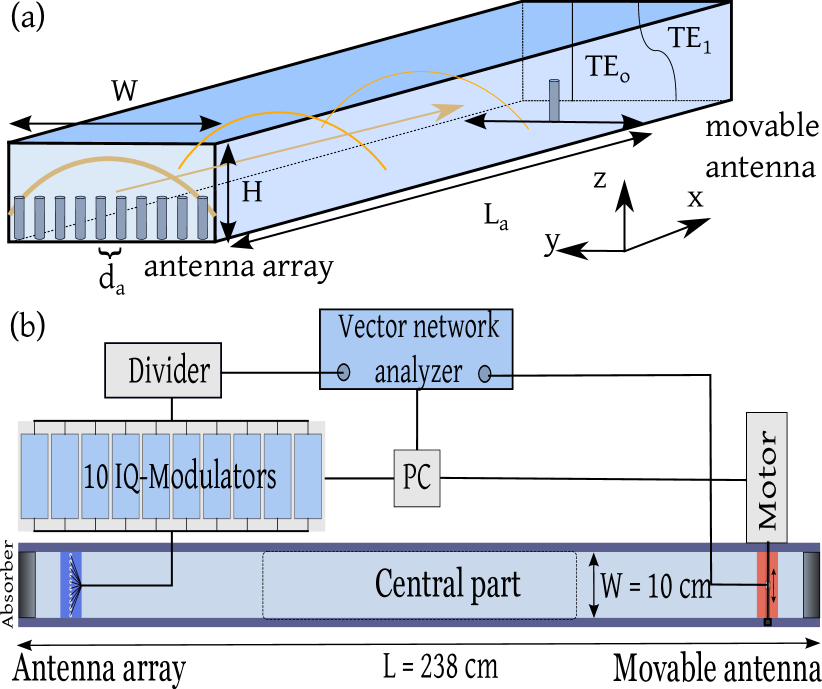
Figure 1: (a) Sketch of the waveguide indicating the antenna array and the movable antenna in a 3D sketch of a rectangular waveguide. The electric field dependence of the TE₀ and TE₁ modes are plotted as well. The height $H$=8 mm. The antennas are monopole antennas introduced via small holes into the waveguide. (b) The experimental setup including the PC, Vector Network Analyzer (VNA), cables, Power divider, IQ-Modulators, and the Q1D waveguide.

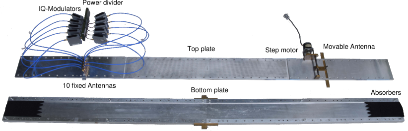
Figure 2: A photograph of the experimental setup showing the exciting 10 antennas with their connection to the power divider via the IQ-Modulators. The top plate is moved from the bottom part to give a view of the interior of the waveguide showing the absorbers at both ends. The holes in the central region of the top plate make it possible to scan the field inside this region.

In this study we use an experimental setup that allows us to measure microwave transport through a multimode metallic-wall waveguide (see fig. 1(a)), where scatterers of different type can be placed. The waveguide has a height of $H=8$ mm, a width $W=10$ cm, a total length $L=2.38$ m and a length between the antenna $L_{a}=1.50$ m thus meeting the waveguide condition

$$H\ll W\ll L.$$ (1)

The quasi one-dimensional setup has been used to investigate the propagation of modes in correlated disordered systems Dietz et al. (2011, 2012a, 2012b), using a second movable antenna instead of the antenna array. In an empty rectangular waveguide the electromagnetic field can be separated into two components of different polarization: the TM polarization with a transverse magnetic field and the TE polarization with a transverse electric field Jackson (1962). To ensure only a single mode in $z$ direction all measurements are performed below the cut-off frequency $\nu_{\textrm{cut}}=c/2H\approx 18.75$ GHz. In this case only the lowest TE-component, having the electric field stretched along the $z$ axis and the magnetic field being in the $(xy)$ plane (see the coordinate system in fig. 1), can propagate.

The input (transmitting) antenna array is excited by a vector network analyzer (Agilent E5071C) via a power splitter (Microot MPD16-060180) and IQ vector-modulators (GTM 1 M2L-68A-5 of GT Microwave Inc). The IQ-modulators can be controlled by a PC and vary the phase and amplitude in the frequency range of 6-18 GHz. The field transmitted by each individual antenna can be adjusted by the corresponding IQ-Modulator, thus the ensemble excites a combination of propagating modes (see also photograph shown in fig. 2). It is worth noting that phase and amplitude control via the IQ-Modulators is broad band meaning that inducing an additional phase shift of $\Delta\phi$ and a relative amplitude reduction of $a$ is valid over the full operating range of the IQ-modulator. $\Delta\phi$ and $a$ have a 12bit control and broad band stability of $\pm 2^{\circ}$ and $\pm 1$ dB.

The output (receiving) monopole antenna is plugged into the waveguide via a slide that can be shifted stepwise by a motor (see fig. 2). Absorbers are placed on both ends of the waveguide in order to reduce reflections from the ends. The used absorbers are ECCOSORB LS-14 and LS-16 with a relative impedance of 0.89 and 0.87 at 10 GHz, respectively. The LS-14 is placed first in direction of the system and has a sawtooth form with 5 teeth in the $y$-direction and a sawtooth depth of about 3.5 cm. Its length is 8 cm and thereafter the second absorber is placed using a linear interface and has a length of 14 cm (for details see fig. 2). Both absorber fill the full height over the full width. It is important to note that the absorbers at the end are placed sufficiently far away from the antennas to suppress evanescent coupling between antenna and absorbers. In our case the distance is about 2.5 times the width $W$. In the central region additional dielectric or metallic scatterer can be placed to include a scattering system.

III Individual Antenna Excitation

Let us assume for the moment that within the antenna array the other antennas can be neglected. Thus we treat the input antenna 1 as a point source, while the output antenna 2 is an observation point. We will follow the description and notation of Dietz et al. (2010). The electric field of a point source is determined by the retarded Green’s function ${\cal G}(|x-x^{\prime}|;y,y^{\prime})$. The Green’s function for the empty waveguide in the normal-mode representation reads

$${\cal G}(|x-x^{\prime}|;y,y^{\prime}) = \sum_{n=1}^{N_{W}}A_{n}\sin\left(\frac{\pi ny}{W}\right)\sin\left(\frac{\pi ny^{\prime}}{W}\right)$$ (2)

$$\times\frac{\exp\left(ik_{n}|x-x^{\prime}|\right)}{ik_{n}W}.$$

Here we introduced the factor $A_{n}$ which effectively describes the coupling between the antennas and normal modes labeled by index $n$. The quantities $\pi n/W$ and $k_{n}$ are, respectively, the discrete values of transverse, $k_{y}$, and longitudinal, $k_{x}$, wave numbers:

$$k_{n} = \sqrt{k^{2}-\left(\frac{\pi n}{W}\right)^{2}}=\frac{2\pi}{c}\sqrt{\nu^{2}-(n\nu_{c})^{2}},$$

$$\textrm{with}\ n=1,2,3,\ldots,N_{W}.$$

Here $k=2\pi\nu/c$ is the total wave number for the electromagnetic wave of frequency $\nu$. The total number $N_{W}$ of propagating waveguide modes is determined by the integer part $\left\langle\ldots\right\rangle$ of the mode parameter $kw/\pi=\nu/\nu_{c}$,

$$N_{W}=\left\langle kW/\pi\right\rangle=\left\langle\nu/\nu_{c}\right\rangle.$$ (4)

Correspondingly, the sum in eq. (2) runs only over the propagating modes with $n\leq N_{W}$ and ignores the contribution of evanescent modes for which $n>N_{W}$. Indeed, for evanescent modes the values of $k_{n}$ are purely imaginary; therefore, they do not contribute to the transport. The critical frequency for the $n$th mode

$$\nu^{(n)}_{c}=nc/2W,$$ (5)

below it is evanescent.

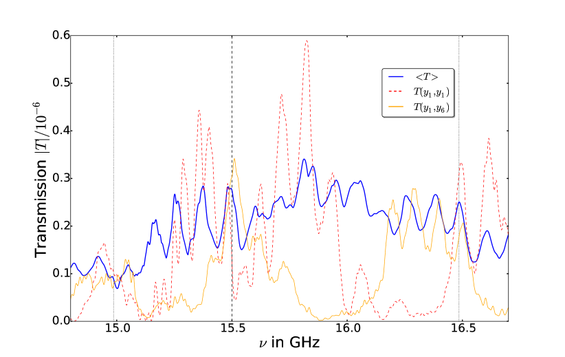
Figure 3: Transmission for different antenna positions $y_{1}$ and $y_{2}$ and its mean value $\langle T\rangle$ as a function of frequency, where the average was taken over all positions $y_{1}$ and $y_{2}$.

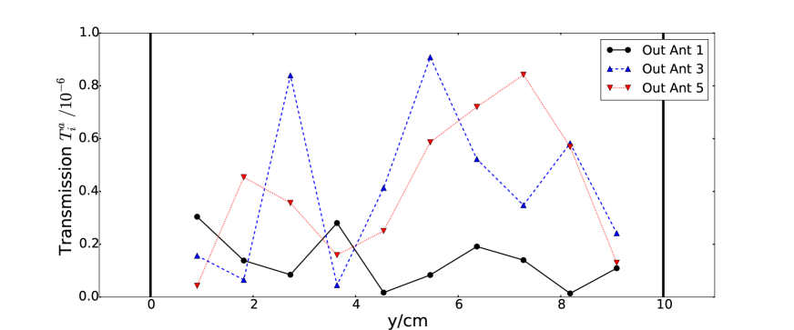
(a)

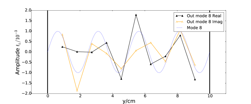
(b)

Figure 4: (a) Measured transmission intensity $T^{a}_{ij}$ from different input antennas $i$ of the antenna array to the movable antenna at position $y_{j}$ at 15.5 GHz. (b) Real and imaginary parts of the transmission amplitudes $S_{nm}$ of the 8th mode (using eq. (6)) to the movable antenna at 15.5 GHz. The dashed line corresponds to the 8th mode. A global phase shift to the data was performed such that the averaged imaginary part is 0.

In this paper we will concentrate on the range $15\leq\nu/$GHz$\leq 16.5$ where 10 modes can freely propagate. The transmission through the rectangular waveguide for two different antenna positions and its averaged value is shown in Fig. 3. The wave front shaping is adjusted at 15.5 GHz.

The scattering matrix $S$ in the modal representation for the whole waveguide ($|x-x^{\prime}|=L$) can be described as the twofold sine-Fourier transform,

$$S_{nm}=\frac{2}{W}\int\limits_{0}^{W}\textrm{d}y\textrm{d}y^{\prime}\sin\left(\frac{\pi ny}{W}\right)\sin\left(\frac{\pi my^{\prime}}{W}\right){\cal G}(L;y,y^{\prime}).$$ (6)

One can see that in accordance with eq. (2) the scattering matrix for the empty quasi-1D waveguide eq. (6) is diagonal in the mode representation.

For the experimental data analysis, the continuous Fourier transform eq. (6) is replaced by its discrete counterpart, allowing us to compute $S_{nm}$ from ${\cal G}(L;y,y^{\prime})$ measured for different positions $y$ and $y^{\prime}$ of input and output antennas. An example of the transmission at 15.5 GHz is shown in fig. 4. In (a) the transmission intensity of a single antenna excitation of the input array is shown as a function of the output antenna position for three different input antennas. In (b) we use eq. (6) to excite only the 8th mode of the cavity. As in the rectangular waveguide the 8th mode is freely propagating we expect to see the 8th mode only. Clearly we do not observe only the 8 mode, but a superposition of several modes. The relative proportion of the 8th mode is 64% of the total intensity. Have in mind that using the same kind of scanning antenna eq. (6) is valid and have been used to investigate correlated disorder in quasi one-dimensional systems Dietz et al. (2011, 2012a, 2012b). This effect is due to the presence of the other antennas in the near field, which destroys the simple description eq. (6). In the next section, we will show experimentally that it is still possible to excite all 10 modes individually even for the whole frequency range of 15 to 16.5 GHz, referring exactly to 10 propagating modes.

IV Decomposition in Rectangular Waveguide and Broad Band Characteristics

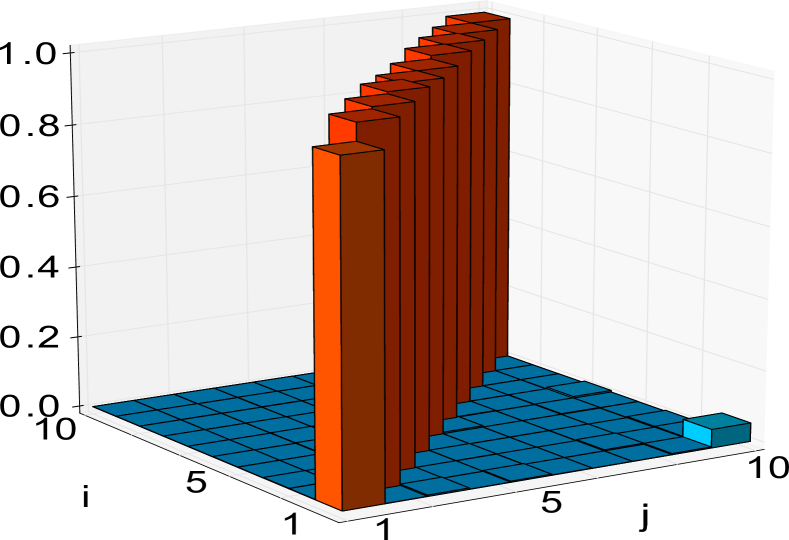
Figure 5: Measured Transmission matrix elements $T_{ij}$ for the rectangular waveguide where $i$ represent the sinusoidal mode number of the input and j the sinusoidal mode number of the output. The input basis have been adjusted by appropriate IQ-modulator phases and amplitudes.

We now measure the transmission of the antenna array to the movable antenna by illuminating each antenna individually. Each excitation of the other antennas are suppressed by about 40 dB using the IQ-modulators (see also fig. 4(a)). By solving a linear equation system for sinusoidal output we calculated the new basis for the input antennas. This calculation yields the phase $\phi_{i}$ and amplitudes $a_{i}$ values to adjust the IQ-modulators. Now we are able to excite exactly the mode of interest. In fig. 5 the transmission matrix $T$ in the sinusoidal input and output basis is shown showing the diagonal matrix.

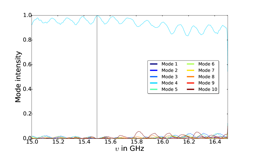
(a)

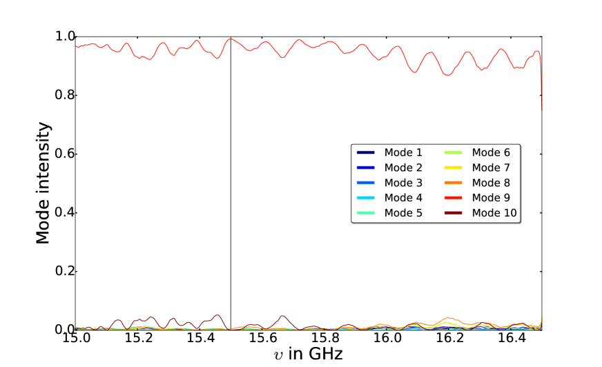
(b)

Figure 6: Measured transmission $T=|t(n_{\mathrm{in}},n_{\mathrm{out}},\nu)|^{2}$ of incident mode $n_{\mathrm{in}}=3$ (a) and 8 (b) as a function of frequency $\nu$. Over the whole range, where 10 modes are supported, mainly the outgoing mode $\mathrm{out}=3$ or 8, respectively, is dominant, even though the adjustment was done for $\nu=15.5$ GHz.

As the IQ-modulators adjust the phase and amplitudes in the whole frequency range from 6 to 18 GHz and we have taken care of using the same cables, connectors, antennas, so the phase shifts for all antennas should be the same over a broad frequency range. In fig. 6 we present the transmission of input mode 3 (a) and 8 (b) into all modes over the frequency range supporting exactly the 10 modes. On the one hand side one observes that at the adjustment frequency 15.5 GHz the modes 3 and 8 are very close to 1, respectively. Apart from that, mode 3 (8) are still very dominant in the whole range presented.

V Decomposition with Scattering region

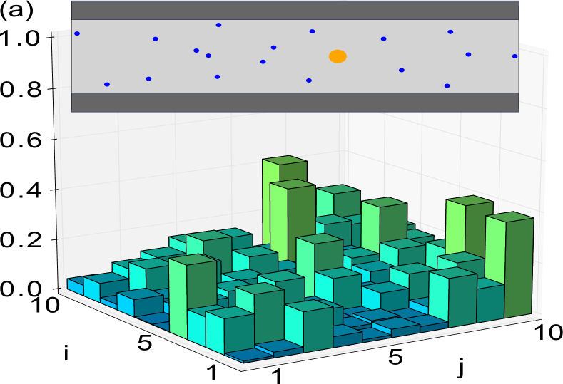
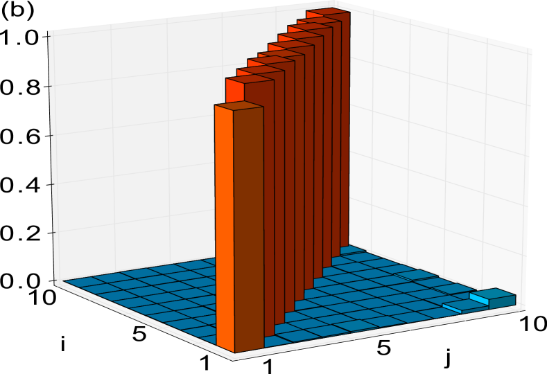
Figure 7: Introducing a scattering region with 18 teflon cylinders with $r=2.5$ mm (blue filled circles in the inset) and with a larger brass cylinder with radius $r=8.85$ mm (orange filled circle in the inset) a single mode excitation $n_{\mathrm{in}}$ is scattered into many outgoing channels $n_{\mathrm{out}}$ (see upper part). Readjusting the incoming wave front to a single outgoing mode $n_{\mathrm{out}}$ can be created.

Now we include a scattering region inside the rectangular waveguide (see inset fig. 7(a) and fig. 1(b)), where we place 18 dielectric (Teflon) scatterers with radius 2.5 mm and a larger brass scatterer inside the central region. Figure 7(a) shows the transmission matrix $T$ in the sinusoidal input and output basis. The scatterers distribute the incoming modes into several outgoing modes. Using this scattering information one can readjust the incident basis in such a way that we get single sinusoidal modes on the outgoing part, leading to a diagonal transmission matrix $T^{\prime}$, where the ^′ indicates the change of basis (see Figure 7(b)).

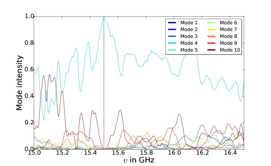
(a)

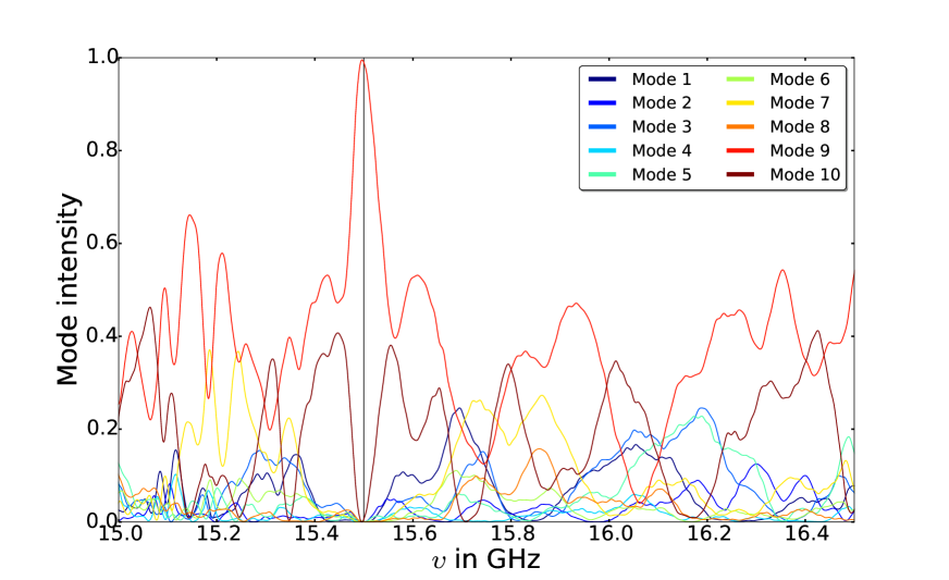
(b)

Figure 8: Measured transmission $T^{\prime}=|t(n^{\prime}_{\mathrm{in}},n_{\mathrm{out}},\nu)|^{2}$ of incident mode $n^{\prime}_{\mathrm{in}}=3$ (a) and 8 (b) as a function of frequency $\nu$. Over the whole range, where 10 modes are supported. The outgoing mode $\mathrm{out}=3$ or 8 are still dominant close to the adjustment frequency $\nu=15.5\,GHz$. But in case of the 8th mode it decays rapidly loosing the broad band features whereas mode 3 stays dominant over a broader frequency range.

Depending on the scattering system certain outgoing modes might be still rather broad band. This can be seen in fig. 8, where the 8th mode is very narrow but the $n_{\mathrm{out}}=3$ mode is still broad, even though not comparable to the situation observed in the rectangular waveguide (see fig. 6). Note that it is important that the scattering systems transmits sufficiently and localization effects are still weak. If the scattering system has not sufficient transporting modes, i.e. the transporting modes are smaller then the number of outgoing modes, a full control will not be feasible. In the case of strong localization the control of the outgoing mode by incident wave shaping is totally lost as the outgoing mode is solely defined by a single transporting mode Peña et al. (2014).

VI Conclusion

In this paper we have shown that it is possible to make broad band wave front shaping within a multi mode waveguide, e.g. a quasi one-dimensional rectangular waveguide, by using IQ-modulators and monopole antennas. The fact, that the antennas are situated in the near field of each other does destroy the use of sine transforms to adjust the IQ-modulators. However, full potential of wave front shaping is accessible if the far field scattering matrix of each individual antenna is known by measurement. We were even able to perform the incident wave shaping in such a way that the wave after undergoing scattering shows a pure sinusoidal mode profile. Attaching the quasi one-dimensional channel including the antenna array with the IQ-modulators to different kind of systems gives the possibility to enhance transmission, realize particle like scattering states, create coherent perfect absorbers and focus microwaves on sub wave length scales as already indicated in the introduction.

References

- Yu (2003) Wei Yu, “Spatial multiplex in downlink multiuser multiple-antenna wireless environments,” in Global Telecommunications Conference, 2003. GLOBECOM ’03. IEEE, Vol. 4 (2003) pp. 1887–1891 vol.4.
- Vellekoop and Mosk (2008) I. M. Vellekoop and A. P. Mosk, “Universal optimal transmission of light through disordered materials,” Phys. Rev. Lett. 101, 120601 (2008).
- Vellekoop et al. (2010) I. M. Vellekoop, A. Lagendijk, and A. P. Mosk, “Exploiting disorder for perfect focusing,” Nat. Photon. 4, 320 (2010).
- Aubry et al. (2003) J.-F. Aubry, M. Tanter, M. Pernot, J.-L. Thomas, and M. Fink, “Experimental demonstration of noninvasive transskull adaptive focusing based on prior computed tomography scans,” J. Acoust. Soc. Am. 113, 84 (2003).
- Rotter et al. (2011) S. Rotter, P. Ambichl, and F. Libisch, “Generating particle like scattering states in wave transport,” Phys. Rev. Lett. 106, 120602 (2011).
- Chong et al. (2010) Y. D. Chong, L. Ge, H. Cao, and A. D. Stone, “Coherent perfect absorbers: Time-reversed lasers,” Phys. Rev. Lett. 105, 053901 (2010).
- Gmachl (2010) C. F. Gmachl, “Laser science: Suckers for light,” Nature 467, 37 (2010).
- Wan et al. (2011) W. Wan, Y. Chong, L. Ge, H. Noh, A. D. Stone, and H. Cao, “Time-reversed lasing and interferometric control of absorption,” Science 331, 889 (2011).
- Pendry (2008) J. B. Pendry, “Light finds a way through the maze,” Physics 1, 20 (2008).
- Gérardin et al. (2014) B. Gérardin, J. Laurent, A. Derode, C. Prada, and A. Aubry, “Full transmission and reflection of waves propagating through a maze of disorder,” Phys. Rev. Lett. 113, 173901 (2014).
- Hsu et al. (2015) C. W. Hsu, A. Goetschy, Y. Bromberg, A. D. Stone, and H. Cao, “Broadband coherent enhancement of transmission and absorption in disordered media,” Phys. Rev. Lett. 115, 223901 (2015).
- Derode et al. (2001) A. Derode, A. Tourin, and M. Fink, “Random multiple scattering of ultrasound. II. Is time reversal a self-averaging process?” Phys. Rev. E 64, 036606 (2001).
- Lerosey et al. (2006) G. Lerosey, J. de Rosny, A. Tourin, A. Derode, and M. Fink, “Time reversal of wideband microwaves,” Appl. Phys. Lett. 88, 154101 (2006).
- Lerosey et al. (2007) G. Lerosey, J. de Rosny, A. Tourin, and M. Fink, “Focusing beyond the diffraction limit with far-field time reversal,” Science 315, 1120 (2007).
- Dupré et al. (2016) M. Dupré, F. Lemoult, M. Fink, and G. Lerosey, “Exploiting spatiotemporal degrees of freedom for far field subwavelength focusing using time reversal in fractals,” Preprint (2016), arXiv:1603.01725.
- Dietz et al. (2011) O. Dietz, U. Kuhl, H.-J. Stöckmann, N. M. Makarov, and F. M. Izrailev, “Microwave realization of quasi-one-dimensional systems with correlated disorder,” Phys. Rev. B 83, 134203 (2011).
- Dietz et al. (2012a) O. Dietz, U. Kuhl, J. C. Hernández-Herrejón, and L. Tessieri, “Transmission in waveguides with compositional and structural disorder: experimental effects of disorder cross-correlations,” New J. of Physics 14, 013048 (2012a).
- Dietz et al. (2012b) O. Dietz, H.-J. Stöckmann, U. Kuhl, F. M. Izrailev, N. M. Makarov, J. Doppler, F. Libisch, and S. Rotter, “Surface scattering and band gaps in rough waveguides and nanowires,” Phys. Rev. B 86, 201106(R) (2012b).
- Jackson (1962) J. D. Jackson, Classical Electrodynamics (Wiley, New York, 1962).
- Dietz et al. (2010) B. Dietz, H. L. Harney, A. Richter, F. Schäfer, and H. A. Weidenmüller, “Cross-section fluctuations in chaotic scattering,” Phys. Lett. B 685, 263 (2010).
- Peña et al. (2014) A. Peña, A. Girschik, F. Libisch, S. Rotter, and A. A. Chabanov, “The single-channel regime of transport through random media,” Nat. Commun. 5, 3488 (2014).