The ExoMol project: Software for computing large molecular line lists
Abstract
The use of variational nuclear motion programs to compute line lists of transition frequencies and intensities is now a standard procedure. The ExoMol project has used this technique to generate line lists for studies of hot bodies such as the atmospheres of exoplanets and cool stars. The resulting line list can be huge: many contain 10 billion or more transitions. This software update considers changes made to our programs during the course of the project to allow for such calculations. This update considers three programs: Duo which computed vibronic spectra for diatomics, DVR3D which computes rotation-vibration spectra for triatomics, and TROVE which computes rotation-vibration spectra for general polyatomic systems. Important updates in functionality include the calculation of quasibound (resonance) states and Landé -factors by Duo and the calculation of resonance states by DVR3D. Significant algorithmic improvements are reported for both DVR3D and TROVE. All three programs are publically available from ccpforge.cse.rl.ac.uk. Future developments are also considered.
Graphical Table of Contents
Molecular spectra provide important remote sensing fingerprints. However hot molecules can undergoing very large numbers of possible transitions: billions for even fairly small molecules such as methane. Nuclear motion software based on the use of the variational principle used to compute line lists is discussed and the adaptation of the programs to the demands of computing huge lists of molecular transitions described.
1 Introduction
The ExoMol projects aims to compute line lists of molecular transitions which are important for the study of hot atmospheres, particularly those of exoplanets, brown dwarfs and cool stars.1 In practice these line lists are also useful for a variety of terrestrial applications as well as for models of non-thermal environments such as masers. The project has produced comprehensive line lists for a number of molecules including BeH, MgH and CaH 2, SiO 3, HCN/HNC 4, CH4 5, NaCl and KCl 6, PN 7, PH3 8, H2CO 9, AlO 10, NaH 11, HNO3 12, CS 13, CaO 14, SO2 15, HOOH 16, H2S 17, SO3 18, VO 19, H 20 and CrH 21; the diatomic studies generally include consideration of all important isotopologues. These line lists are large with, for example, the line list for the diatomic 40Ca16O containing over 28 million transitions 14, and those for the polyatomic systems CH4, PH3, H2CO, HOOH and SO3 containing 10 billion or more lines. These calculations can also be used for other purposes such computing radiative lifetimes of individual states22 and thermally-averaged properties.
Computing these line lists has led us to develop or improve specialist programs designed to study the nuclear motion problem of the various molecules under consideration. This software update describes these developments. A common theme of all these programs is the direct solution of the nuclear motion Schrödinger equation using a variational treatment. In the next section we outline the overall methodological approach adopted by ExoMol. In the following sections we consider the main programs used under the project. They are grouped by the type of system studied. Section 3 considers diatomic systems, for which we use Le Roy’s program Level 23 and our program especially developed for the project, Duo.24 Unlike the other programs considered here, Duo is designed for the calculation of vibronic spectra and can treat problems involving coupled potential energy curves. Section 4 considers triatomic systems for which the exact kinetic energy nuclear motion code DVR3D 25 has been employed. For tetratomic systems calculations have largely been performed with TROVE 26 although WAVR4 27 has also been tested.28 TROVE, which has also been used to study methane, will be considered in section 5. Finally a new hybrid methodology based on the combined use of the variational principle and perturbation theory has been developed for larger systems. This will be considered in section 6. The final section considers our conclusions and prospects for the future.
A number of other groups are involved in projects computing extensive molecular line lists for astronomical or other purposes, again largely using especially developed software for the nuclear motion problem. These include the NASA Ames group of Huang, Schwenke and Lee who use the polyatomic nuclear motion program VTET 29 and have also been undertaking theoretical developments.30 Tyuterev and Rey from the University of Rheims in collaboration with Nikitin from the Tomsk Institute of Atmospheric Optics have computed line lists for a number of polyatomic species31, 32 using either their variational polyatomic code or contact transformation approach. Bowman’s group has developed a very efficient general approach to compute ro-vibrational intensity of polyatomic molecules using MULTIMODE 33 which has also been used to generate hot line lists.34 Finally, we note that Bernath’s group has produced a number of diatomic line lists based on the use of level with the effects of electron spin treated using perturbation theory 35, 36, 37. We note that there are also a number of studies which are the product of collaboration between the various groups.6, 15, 38
2 Method
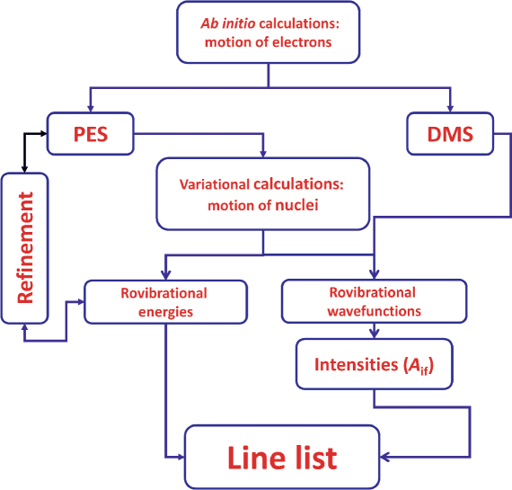
The general methodology used by us for constructing line lists has been extensively discussed elsewhere; in particular Lodi and Tennyson 39 gave an introduction on how to perform such calculations and Tennyson 40 reviewed the methodology used by the ExoMol project which is summarised in Fig. LABEL:f:workflow.
The first step in the calculation is construction of a potential energy surface (PES) using a high-level, ab initio procedure, which we generally do with MOLPRO 41. At the same time the computation of the appropriate dipole moment surfaces (DMS) is performed. These then form the input to the appropriate nuclear motion program; these programs are the focus of the present article. In only a very few cases 42, 43, 44, 20 are completely ab initio procedures the best choice for obtaining an accurate line list. In general this is only true for systems with very few electrons. Otherwise it is necessary to refine the calculation using experimental data.
There are three methods of improving the calculated line list on the basis of empirical data. The most common one is to refine the PES in the manner illustrated in Fig. LABEL:f:workflow. This methodology, which is widely used by a number of groups, 45, 46, 47 involves either adjusting parameters in the original fit of the PES or adding an auxiliary function which captures changes to this PES. The second method, which can only be used in programs such as TROVE which uses uncoupled vibrational and rotational basis functions, the so-called representation of rotational excitation 48, involves band origin shifts. In this method, the vibrational band origins that are computed in the rotationless () step of the calculation can be shifted to the observed one prior to solving the fully-coupled rotation-vibration problem 48. The third method involves substituting empirical energy levels at the end of the calculation. The format used for storing ExoMol line lists 49, 50 involves creating a states file which contains all energy levels and associated quantum numbers. There are now well-established procedures for extracting experimentally-determined energy levels from high resolution spectra 51, 52, 53, 54 and these energies can simply be used to replace the computed ones in the states file.
The situation with DMS is very different. The evidence is that DMS can be calculated ab initio more accurately than they can be obtained by inverting experimental data 55. Furthermore theoretical procedures have been developed which allow the assignment of uncertainties to individual transition intensities 56, 57, although at present these are too onerous to be used routinely for the very large line lists being considered here. Reviews discussing the theoretical determination of accurate DMS have been given by each of us 58, 59.
The nuclear motion programs which are the focus of this software review can be thought of as solving the Schrödinger equation implied by the nuclear-motion Hamiltonian:
| (1) |
where runs over the coordinates of the nuclei, each of mass , and is the PES expressed in internal coordinates . Of course this expression already assumes the Born-Oppenheimer approximation and neglects any couplings between PESs. To make progress with Hamiltonian (1) it is necessary to separate out the centre-of-mass coordinates which represent the translation motion of the whole molecule. The methods below also all work in body-fixed coordinates which involve separating the rotations from the vibrations by fixing an axis system to the molecular frame and using internal coordinates to express the vibrational coordinates. Precisely how this is done varies between the different programs.
In the standard variational approach the energies and wave functions of the body-fixed Hamiltonian are obtained by using appropriate basis functions to represent the rotational and vibrational motion, and then diagonalizing the resulting matrix; see, for example, the review by Bowman et al. 60. For the rotational motions the choice of basis functions is straightforward as symmetric top eigenfunctions (Wigner -matrices) form a complete set. For the vibrational coordinates it is often preferable to use a grid-based discrete variable representation (DVR) 61 rather than actual functions. Furthermore, rather than diagonalizing the resulting Hamiltonian matrix in a single step, our approach often uses intermediate diagonalizing steps so that the final matrix diagonalization is as compact as possible.
Ones ability to diagonalize the large matrices necessary for obtaining the many energies and wave functions required for computing hot line lists usually provides the computational bottleneck in these calculations. However, the very large number of transition probabilities, which we generally choose to represent as Einstein A coefficients, that need to be computed usually means that this step can come to dominate the actual computer time used. Measures to mitigate this are discussed below.
3 Diatomics systems
Le Roy’s program LEVEL 23 is our choice for computing the spectra of closed shell () diatomic molecules. The program has been refined over many years by Le Roy and has been used by us without further changes.
However, for more complicated diatomic systems, in particular ones involving coupled electronic states or non- states, we have developed our own program, Duo. A first release of Duo has just been published 24 and the reader is refered to this paper and an associated topical review 62 for full details. Duo is still under regular development and a number of improvements to the functionality of the published version have been made of which we highlight three here.
First, the published version of Duo only considers truly bound states. However, there are a number of situations where it is necessary to consider quasi-bound or resonance states, or indeed the continuum itself. Shape resonances arise when rotational excitation leads to quasi-bound states being trapped by the centrifugal barrier. There are also Feshbach resonances which undergo pre-dissociation caused by coupling to dissociative states. Finally, it is sometimes necessary to consider spin-orbit effects on bound states caused by coupling to either resonances or the continuum. A facility has been added to Duo which allows an artificial wall to be placed at large internuclear separation; this has the effect of discretizing the continuum and allowing localized, resonance states to be identified 63.
Second, the energy levels of open shell molecules are sensitive to the effects of magnetic fields. The behaviour of molecules in a magnetic field provides a spectroscopic tool as well as being important in fields as diverse as molecular trapping 64 and astrophysics 65. For an open shell diatomic, the splitting, , due to weak magnetic field of strength , otherwise known as the Zeeman splitting, is given by
| (2) |
where is the total angular momentum quantum number and is its projection along the direction of the magnetic field. Here is the effective Landé g-factor for the given level and is the Bohr magneton. In simple cases can be evaluated in the Hund’s case (a) basis used by Duo, using the expression
| (3) |
where and are the orbital and spin -factors respectively. In eq. (3), is the eigenvector of the state with good quantum numbers and (parity) and is a compound basis index
| (4) |
In this ‘state’ denotes an electronic state with electron spin and an associated vibrational state. , and are projection of the orbital angular momentum and spin, , onto the body-fixed molecular axis, respectively. In Eq. (3), and are subscripted by to emphasize that they are not conserved quantities but their value depends on the state part of the basis. Berdyugina and Solanki65 give a more complete expression for which allows it to be evaluated correctly using Duo wavefunctions even when the molecule is not well-represented by Hund’s case (a). An extension to Duo to evaluates this general expression has recently been written and tested for a few diatomic systems, notably CrH, C2 and AlO.66
Finally, visualization of wave functions can be very helpful for interpreting results. The latest version of Duo has incorporated plotting routines to aid the inspection of the results.
4 Triatomic systems
The DVR3D program suite obtains variationally exact solutions for the bound-state, three-atom nuclear motion problem for a given PES within the Born-Oppenheimer approximation. The program has been developed over a number of years originally starting as a finite basis set procedure 67, 68, 69, 70 before evolving 71 to one which is based on the use of DVR in all vibrational coordinates 72, 73. DVR3D and its predecessors have been benchmarked against other, similar, nuclear motion codes such VTET, and indeed TROVE, to confirm the accuracy of both the computed vibration-rotation energy levels 74, 15 and transition moments 75.
The current published release of the DVR3D program suite 25 is actually the third but dates back to 2003. Since then DVR3D has undergone a large series of developments, not least to facilitate the calculation of huge line lists. All modules have also been subject to a re-write to both make them more consistent and to bring the programming up to a more modern programming standard.
Figure LABEL:f:dvr3d gives the flow structure for the current version of DVR3D. The main driving module, DVR3DRJZ, solves the vibration-only or Coriolis-decoupled vibration-rotation problem. For rotationally-excited molecules, the results of DVR3DRJZ provide the basis functions used in one of the ROTLEV modules to solve the fully-coupled vibration-rotation problem; where the choice of module depends on the axis embedding used. The solutions to vibration-rotation problem can be used to compute expectation values of given variable in XPECT, this module is particularly used in performing fits of the PES to spectroscopic data where the Hellmann-Feynman theorem can be used to evaluate the expectation values of derivatives of the PES with respect to parameters of the fit. These same vibration-rotation eigenvectors can be used to compute line strengths in DIPOLE which in turn provides the necessary information to generate spectra. The new modules and significantly amended modules have been highlighted in this figure and are discussed below.
A new module, RES3D, has been written 76 which can be used to characterize quasibound or resonance states lying above dissociation. The automated procedure for doing the analysis has been successfully used to study resonances in both H 76 and water 77. Details of how this module works are given below.
In addition the functionality of DVR3D has been increased by a thorough re-write of the codes in which the -axis is placed perpendicular to the plane of the molecule (-perpendicular embedding option 78, 79). This option is useful for molecules, such as H, whose projected rotational motion is usually quantised along this axis. A new module, DIPOLE3Z, is introduced which computes transition dipoles for the -perpendicular embedding case.
Algorithmic improvements include the following:
-
•
The automated Gauss-(associated) Legendre quadrature generation procedure, which was adapted from one given by Stroud and Secrest 80 has been replaced by a brute force one which involves finding zeros in the polynomial equation for the point quadrature. This was found to be essential for grids with and has been successfully used for up to 150 15. The automatic check on the validity of grid obtained by comparing summed weights with the analytic value given by Stroud and Secrest has been retained.
-
•
For large calculations, module ROTLEV3b in the published version of DVR3D can spend a long time constructing the final Hamiltonian matrix. ROTLEV3b uses vibrational functions generated in the first step of the calculation 81 to provide basis functions for the full ro-vibrational calculation performed by ROTLEV3b. For high calculations this algorithm involves transforming large numbers of off-diagonal matrix elements to the vibrational basis set representation, see Eq. (31) in Tennyson and Sutcliffe 82. This step has been re-programmed as two successive summations rather than a double summation at the cost of requiring an extra, intermediate matrix 17. This had the effect of reducing the cost of Hamiltonian construction to below that of Hamiltonian diagonalization, which is generally the case for the other modules of DVR3D.
-
•
Dipole3 by default computes all transition dipoles between the bra and ket wave functions it is asked to process. For large line lists, computing transition dipoles actually dominates computer usage and this can be inefficient. These line lists are usually characterized by a lower energy cut-off, which determines the temperature range for which the line list is valid, and an upper energy cut-off which determines the frequency range. Computing transition moments between these ranges is expensive and unnecessary. New input variables have been introduced to avoid this 83.
-
•
DVR3DRJZ employs an algorithm which relies on solving a Coriolis-decoupled vibrational problem for each , where is the projection of the rotational angular momentum onto the chosen body-fixed axis and is the rotational motion quantum number. This provides a basis set from which functions used to solve the fully-coupled ro-vibrational problem are selected on energy grounds 80. Hot line list can involve calculations with high and experience has shown that in this case not all combinations are actually needed. An option has been implemented where unneeded high calculations are not performed 15. In practice, this does not save much computer time, since the initial calculations are quick, but does save disk space.
-
•
Again for large calculations, the algorithm used by module DIPOLE3 to read in the wave functions required a lot of redundant reads. DIPOLE3 has been re-structured to reduce the number of times the wave functions need to be read 15.
Finally, matrix diagonalization is the rate-limiting step in most applications of DVR3D. A number of new real, symmetric matrix diagonalizers have been added to the LAPACK software package 84. The diagonalizers implemented in DVR3D have been changed where appropriate.
4.1 Resonance detection
Resonances can be detected by the behaviour of states lying in the continuum upon the introduction of a complex absorbing potential (CAP). To do this the dissociating system’s PES is augmented with a complex functional form that absorbs the continuum part of the wave function. This non-Hermitian Hamiltonian produces wave functions above the dissociation threshold that represent the resonant states in question 85.
Formally, an imaginary negative potential that acts on the dissociation coordinate, , is added to the system’s Hamiltonian, :
| (5) |
where is a parameter used to control the CAP’s intensity. The resulting non-Hermitian Hamiltonian, , defines the energy of the resonance, , its width, , and the corresponding wave function, , through the relationship:
| (6) |
To solve Eq. (6), can be projected on a suitable basis set and diagonalized. In the infinite basis set limit, the eigenvalues corresponding to the resonant states will be found in the limit where . Fortunately the use of a finite basis set is both necessary and beneficial: the error introduced by the CAP and the finite basis set have opposite phase. This implies that these errors will cancel each other out at some optimal value, , thus yielding the complex “observables” associated with the resonant state.
The wavefunctions, , satisfying eq. (6) are naturally complex. This represents both transmission and reflection at the CAP. Theoretically it is best to minimize reflection 86, which can be done by judicious choice of absorbing potential 87. However, our calculations did not find much sensitivity to actual choice of CAP used.76, 88 However, the width in particular is found to be sensitive to convergence of the basis set representation employed.89
A search for is made by studying the behaviour of the complex eigenvalues of Eq. (6) with values of ranging from zero to a large arbitrary value. This results in trajectories in the complex plane, each associated with an eigenvalue . Through graphical analysis of these trajectories it is possible to identify the point in the complex plane that corresponds to the optimal value , and hence estimate the value for the position, , and with, , of the resonant state. This graphical method consists of locating cusps, loops and stability points in the eigenvalue trajectory, which are known to occur in positions around the true eigenvalue for the resonances on the complex plane.76, 90
The approach taken in the new RES3D module of DVR3D is to first diagonalize of the system under study and store the basis elements , and eigenvalues lying near dissociation. As one can expand the functions of Eq. (6) onto the basis set obtained from the bound state calculation:
| (7) |
The coefficients , the resonance energies and the resonance widths can then be obtained by diagonalizing the Hamiltonian:
| (8) |
where is the eigenvalue and is the eigenvector obtained from the diagonalization of . For systems with many bound states, wave functions associated with the strongly bound states are not needed when diagonalizing the Hamiltonian so can be dropped. This means that the Hamiltonian matrix is small, easy to construct and cheap to diagonalize which is important as the graphical method relies on many diagonalizations with different values if .
The matrix is complex symmetric matrix which therefore yields the complex eigenvalues needed to characterize both the position and width of the resonance. RES3D uses LAPACK 84 routine zgeev to perform this diagonalization.
5 Polyatomic systems
Code WAVR4 27 provides tetratomic implementation of the DVR-style approach employed in DVR3D. 91 WAVR4 has been tested28 against the alternative polyatomic code TROVE, described below, and found to considerably slower. There are a number of reasons for this. Firstly, DVR methods are diagonal in the potential and coupling appears through the kinetic energy operator. Although it is possible to formulate a DVR in general coordinates92, this is not efficient as it is only in orthogonal or polyspherical coordinates 93 in which the kinetic energy operator has a simple form that can be efficiently evaluated. Secondly, the representation as implemented in TROVE and discussed below has proved highly efficient for calculations on rotationally excited polyatomics. This form is not supported by WAVR4 which employs theory which naturally samples linear geometries 94, 91 where the representation fails.
TROVE is a variational method with an associated Fortran 2003 program to construct and solve the ro-vibrational Schrödinger equation for a general polyatomic molecule of arbitrary structure 95. The kinetic energy operator is constructed as an expansion in terms of internal vibrational coordinates with the expansion coefficients obtained numerically on-the-fly. The energies and eigenfunctions obtained via a variational approach can be used to model absorption/emission intensities (absorption coefficients) for a given temperature as well as to compute temperature independent line strengths and Einstein coefficients 96. The latter is then used as the input to construct molecular ExoMol line lists. TROVE provides an integrated facility for refining the ab initio PES in the appropriate analytical representation 97. Being a general program TROVE requires modules for each molecular type with all individual specifications including descriptions of the molecular structure, internal coordinates, and their symmetry properties. TROVE uses a symmetry adapted product-type basis set representation with an automatic symmetrization procedure 98. The Hamiltonian matrix constructed by TROVE is factorized into symmetry blocks corresponding to different irreducible representations. The molecular symmetry group 99 is used to classify the symmetries of the basis and wave functions. The construction of the ro-vibrational basis set is performed in three steps: (i) the 1D basis set functions are obtained either as numerical solution of 1D Schrödinger equations using the Numerov-Cooley method 100, 61Coxxxx.method or the harmonic oscillator wavefunctions; (ii) Schrödinger equations are solved for reduced Hamiltonians for different types of degrees of freedom connected by symmetry transformations in order to obtain a more compact, contracted basis set; the eigenfunctions of the Schrödinger equation are then contracted and used to form the final ro-vibrational basis set in the representation 48; (iii) the final step involves constructing and diagonalizing the symmetrized ro-vibrational Hamiltonian matrix.
Apart from computing energies and spectra for a series of polyatomic molecules, the program TROVE has being applied to study some of their properties, for example the so-called rotational energy clustering09YuOvTh.SbH3, jt580 or the temperature-averaged nuclear spin-spin matrix elements10YaYuPa.NH3 and isotropic hyperfine coupling constant15AdYaYuJe.CH3.
Even prior to the ExoMol project a number of modifications had been implemented to TROVE subsequent to its original publication 95, which have proved to be important for the project. These include:
The typical TROVE intensity project consists of the following steps:
-
1.
Expansion of the Hamiltonian operator (generating kinetic and potential energy expansion coefficients numerically on-the-fly) as well as of any ‘external’ function (e.g. dipole moment, polarizability, spin-spin coupling or any other property; PES correction used in the refinement process 97);
-
2.
Numerov-Cooley solution of the 1D Schrödinger equations;
-
3.
Eigen-solutions of the reduced Hamiltonian problems;
-
4.
Symmetrization of the contracted eigenfunctions from Step 3 and construction of the symmetry-adapted vibrational basis set ;
-
5.
Calculation of the vibrational matrix of the Hamiltonian operator as well as external functions (e.g. dipole) when required;
-
6.
Diagonalizaitons of the Hamiltonian matrices for each irreducible representation in question;
-
7.
Conversion of the primitive basis set representation (vibrational matrix elements from Step 5) to the representation;
-
8.
Construction of the symmetry-adapted ro-vibrational basis set as a direct product of the eigenfunctions and rigid rotor wavefunctions;
-
9.
Construction of the ro-vibrational Hamiltonian matrices for each and irreducible representation ;
-
10.
Diagonalization of the Hamiltonian matrices and storing eigenvectors for the postprocessing (e.g. intensity calculations) if necessary;
-
11.
For the intensity calculations (line list production), all pairs of the ro-vibrational eigenvectors (bra and ket) from Step 10 (subject to the selection rules as well as to the energy, frequency and thresholds) are cross-correlated with the dipole moment components in the laboratory-fixed frame via a vector-matrix-vector product, where the body-fixed components of the dipole moment from Step 5 are transformed to the -frame using the Wigner-matrices.
The main challenge of the ExoMol project is that very high rotational and vibrational excitations are needed for for accurate descriptions of high-temperature molecular spectra. This in turn requires larger basis sets and therefore larger Hamiltonian matrices, which associated increase of the calculation costs in terms of memory (both RAM and storage) and time. For example, for the SO3 line list 18 with extremely high rotational excitations (up to ) due to the heavy character of the molecule, the size of the Hamiltonian matrices to be solved has to be as large as 400,000400,000, which represents our biggest calculation so far. This is despite the fact that only the smallest matrix ( and symmetries of (M)) had to be considered due to the nuclear spin statistics of 32S16O3. The sheer size of these matrices requires special measures not only on the software side (TROVE), which is discussed below, but also from the hardware. For this example of the 400K400K matrices, the diagonalizations were performed on the Cambridge SMP facilities within the DiRAC II project, using about 1000 cores, 6 Tb of RAM and a specially adapted version of the eigensolver PLASMA plasma by the SGI team for TROVE.
In order to tackle these and other challenges associated with large basis sets and matrix sizes, the following critical modifications of TROVE have been performed.
Checkpointing. The production of a complete line list for a
polyatomic molecule with four and more atoms, takes very long times, longer
than the wall-clock limits of the high performance computers (HPC)
we have access to would allow. Therefore it was
important to implement the so-called ‘checkpointing’ feature
(i.e. storing data required for a restart)
for all calculation steps of the
TROVE protocol, together with a control
mechanism allowing a restart at any computational step. Moreover, the
eigen-coefficients in different representations used at different
stages are also stored in the form of ‘checkpoints’ thus treating them on
the same footing. In order to prevent accidental usage of the wrong
checkpoints, most of these files contain a built-in structure of
‘signatures’ with a header containing some key parameters representing
a TROVE project (expansion orders of the kinetic and potential
energy functions, sizes and types of the basis sets etc) and
control-phrases at the beginning and end of the different sections (e.g.
End Quantum numbers and energies).
Symmetries. Each molecule type in TROVE is represented as a project specifying reference (equilibrium) geometry, definition of the geometrically defined coordinates (GDC), and description of the associated transformation properties of these coordinates as well as of the rigid-rotor wavefunctions used for the rotational basis set. The same molecule type allows different choices of GDC depending on the specifics of the system as well as of the reference geometries, with the reference configuration to be either rigid or non-rigid. The transformation symmetry properties of the rigid-rotor wavefunctions 05YuCaJe.NH3 will vary depending on the choice of the -axis. For example in case of an XY2 molecule, the -axis can be chosen along the bisecting vector or perpendicular to it, which changes the symmetry properties of . For most of the symmetries, the irreducible (symmetry-adapted) combinations of the rigid-rotor wavefunctions are obtained as Wang functions 82Paxxxx.method
| (9) | |||||
| (10) |
Because of this property and the fact that the Hamiltonnian operator is quadratic in terms of the angular momentum operators , , and , the ro-vibrational Hamiltonian matrix has a block-diagonal structure with vanishing matrix elements for .
In the course of the ExoMol project the following new molecular types and corresponding symmetries were implemented: XY4 (, ) jt555, jt572, non-linear and non-rigid X2Y2 ((M), (M), +(M), (M), (M)) 28, 16, linear X2Y2 ((M), (M), ), rigid X2Y4 ((M)).
Euler symmetry. The XY4 is a special case since the simple symmetrization rules given in Eqs. (9) and (10) do not work 11AlLeCa.CH4 due to the additional symmetry axis (1,1,1) required to define its equivalent rotations 99BuJexx.CH4. The adapted basis set is given in this case by a linear combination of basis functions with spanning different values (). To address this problem a new routine for construction of symmetry-adapted rigid-rotor wavefunctions has been implemented. This symmetrization approach is based on the properties of the Wigner functions upon the equivalent rotations of an arbitrary molecular symmetry group (not only ) and only requires the values of the equivalent Euler angles only (see, for example, 11AlLeCa.CH4). As a consequence abandoning the Wang-type structure from Eq. (9) and (10), the ro-vibrational Hamiltonian matrices do not have the block-diagonal structure. Furthermore, matrix elements of the dipole moment components in the laboratory-frame are also less compact. Therefore the corresponding modules in TROVE responsible for the ro-vibrational Hamiltonian and dipole matrix elements had to be modified. More details can be found in our paper presenting our very large hot methane line list known as 10to10. 5
5.1 PES refinement
The TROVE-refinement method 97 is based on the two main features: (i) the eigenfunctions of the ro-vibrational Hamiltonians (usually ) corresponding to the ab initio potential energy function are used as basis functions to solve the Schrödinger equations for the modified potential function during the refinement procedure; (ii) the refined potential energy function is represented as a correction to the ab initio PES as given by
| (11) |
The refined part of the PES is in turn represented as an expansion in terms of the internal coordinates
| (12) |
with the expansion coefficients being varied using the Hellman-Feynmann theorem. The term plays the role of the external function at Step 5. The TROVE refinement project requires the following additional calculation steps after Step 10 in the calculation protocol above
-
11.
The vibrational matrix elements of (for a given approximation) are converted from the representation (Step 7) to the representation of the ab initio ro-vibrational eigenvectors;
-
12.
At each iteration, a set of refined Hamiltonian matrices are constructed and diagonalized;
-
13.
The eigenvalues are compared to the experimental energy levels;
-
14.
The diagonal matrix elements of on these eigenfunctions are computed and used to evaluate the next approximation for ;
-
15.
The fitting iteration steps are repeated until all accuracy or convergence criteria are satisfied.
In order to prevent non-physical distortions of , the refinement is usually constrained to the original ab initio potential function. This is achieved by a simultaneous fit 03YuCaJe.PH3 of the potential parameters to the experimental energies and ab initio potential function evaluated on a grid of (usually 10,000–20,000) geometries. The current TROVE implementation of the refinement approach given by Eqs. (11) assumes that the same functional form (not necessarily polynomial) in Eq. (12) is also used for :
| (13) |
This simplifies the evaluation of the derivatives of diagonal Hamiltonian matrix elements with respect to needed for the least-squares fit via the following property:
where denotes the Hamiltonian operator with all potential parameters set to zero except which is set to one. That is, the same subroutine can be used to evaluate both and . It should be noted however that an independent form for can be also easily implemented if required.
5.2 Curvilinear coordinates
Originally TROVE was based on the expansion in terms of linearized coordinates around an equilibrium geometry in the case of a rigid molecule or a one-dimensional non-rigid reference configuration 83Jensen.method in the case of molecules with one large amplitude motion (e.g. ammonia or hydrogen peroxide). Linearized coordinates are defined as a linear expansion of GDCs in terms of the Cartesian coordinates displacements truncated after the linear term 96. The linearized coordinates have the advantage of simplifying the Eckart conditions 95. Very recently, TROVE has been extended for expansions in terms of geometrically defined (or curvilinear) coordinates. In order to be able to use the Eckart conditions in this case, an automatic differentiation (AD) procedure has been implemented 15YaYuxx.method. Use of the curvilinear coordinates significantly improves the basis set convergence15YaYuxx.method. This method was originally tested on NH3, PH3, CH3Cl and H2CO, and has been used in subsequent applications 15OwYuYa.SiH4, jt612, jt634. AD is a robust numerical method to compute derivatives of arbitrary functions by computer programs.
5.3 Dipole moments
As for the potential energy functions, at least in principle, TROVE accepts any analytical form for the electric dipole moments used for intensity calculations. This is because TROVE re-expands any use-defined function in terms of TROVE internal coordinates (either linearized 95 or curvilinear 15YaYuxx.method) using numerical finite differences. TROVE requires that the corresponding subroutine outputs the dipole moment components for any given instantaneous molecular geometry in Cartesian coordinates. Analytical forms for the following dipole moment functions have been implemented in TROVE: XY3-type molecular bond (MB) 05YuCaLi.NH3 and symmetrized MB representations 09YuBaYa.NH3; an HSOH-type dipole moment function (DMF) 09YuYaTh.HSOH; an H2CS-type DMF 13YaPoTh.H2CS, 9; an XY4-type symmetrized MB representation jt555; an HOOH-type dipole moment function jt638. Since these functions are based on some user-defined choice of the coordinate system, an interface to transform this system to the TROVE coordinates (Cartesian) is always required.
5.4 TROVE for a linear molecule
TROVE was originally written to treat non-linear molecules only. This meant that TROVE was not capable of treating accurately enough for practical spectroscopic applications molecules such as water, which has a relatively low barrier to the linearity. This has been addressed in the most recent version of TROVE by extending it to the so-called - approach, jt22 where the rotation of the molecule around the molecular axis (e.g. ) is excluded from the set of the Euler angles and combined with the set of the vibrational modes. Technically this is done by describing the deformation of the linear geometry (displacement angle) and its rotation about via a double degenerate coordinate (,) representing projections of the bond angle onto the body-fixed and planes. The linearized coordinates in this cases are best suited for this 2D internal mode. All kinetic energy terms corresponding to the component are simply set to zero and thus excluded from the calculations. The construction of the - Hamiltonian requires minimal modifications of the - code. However the ro-vibrational basis set in the product form has to be constrained as follows 70Watson.method
where is the rotational quantum number (projection of the rotational angular momentum on ), are the vibrational angular momenta and is a generic vibrational quantum number. Thus the vibrational basis set has to be constructed with as a ‘good’ quantum number. Full details of our - approach will be reported elsewhere.
5.5 Rotational energy clustering
TROVE has been used to study the effect of the rotational energy clustering 72DoWaxx.cluster for the XY3 type molecules SbH3, BiH3, PH3, AsH3, and SO3 09YuOvTh.SbH3, 14UnYuTe.SO3. In order analyze the associated localization rotations, 96KoPaxx.cluster the following modules were implemented: (i) construction of classical rotational energy surfaces 84HaPaxx.cluster, (ii) construction of rotational probability density 05YuThPa.PH3 and (iii) determination of axes characterized by stable localized rotations.
5.6 Temperature averaging and matrix exponent expansion
For an ensemble of molecules in thermal equilibrium at absolute temperature the thermal average of a molecular property is given by
| (14) |
where is the degeneracy of the th state with the energy relative to the ground state energy, is the Boltzmann constant and is the internal partition function defined as
| (15) |
and is an expectation value of in a rovibrational state
| (16) |
A TROVE module for computing thermal averaging of a general molecular function based on Eqs. (14–16) was implemented and applied to indirect nuclear spin-spin coupling constants and equilibrium structure of of ammonia 10YaYuPa.NH3 and isotropic hyperfine coupling constant of methyl radical 15AdYaYuJe.CH3. The calculations require the ro-vibrational eigenvalues and eigenvectors obtained by a time-consuming matrix diagonalization. An alternative to this (also implemented as a part of this module) is an averaging technique based on the construction of the density matrix obtained by expanding the matrix exponent of a Hamiltonian matrix as a Taylor series:
| (17) |
in the representation of the basis functions. This approach is based on the realization that Eq. (14) represents the trace of a matrix product:
| (18) |
involving the (diagonal) density matrix
| (19) |
Since the trace does not depend on the choice of the representation Eq. (19) is conveniently evaluated in the basis set representation.
5.7 GAIN
The longest part of the line list production is usually the intensity calculations. The hot line lists of polyatomic molecules typically require billions of transition dipoles (linestrengths or Einstein A coefficients) to be computed. A calculation of a linestrength (as well as of an Einstein coefficient) requires a matrix element of the molecular space-fixed dipole moment for all TROVE ro-vibrational eigenfunctions subject to the selection rules and thresholds (see TROVE protocol above), i.e. a vector-matrix-vector product, each of which is relatively small in terms of the memory costs and fully independent from other transitions. This makes it perfectly suitable for the GPU architecture. We have modified the intensity part of TROVE to make it compatible for and efficient with GPUs. The new TROVE module and the underlying approach is called GAIN jtGAIN. With small modifications GAIN could be adopted for other variational programs. The gain in the calculation speed is from a factor of 10 to 1000 depending on the type of GPU used.
6 Larger molecules
As part of the ExoMol project we have worked with one further nuclear motion code AngMol which was originally developed by Gribov and Pavlyuchko 88GrPa.method. With Pavlyuchko we developed a hybrid variational – perturbation theoretical method for treating both vibrational and vibrational-rotational motion jt588 and computing spectra of large, hot systems efficiently jt603. This methodology has been used successfully to obtain a line list for hot nitric acid (HNO3) 12. However, AngMol has been developed in a highly specific manner. Rather than continuing its development, our plan is to implement the hybrid procedure successfully tested in AngMol within TROVE.
7 Conclusions and future developments
The codes Duo, DVR3D and TROVE are all publicly accessible via the CCPForge program depository (https://ccpforge.cse.rl.ac.uk/), where each of them are available as a separate project.
A number of developments of these codes are in progress or being planned. In particular, we are just starting to extend the polyatomic codes to include transitions between different electronic states and hence to consider the vibronic transitions already considered by the diatomic code Duo. The calculation of all states up to dissociation for strongly-bound triatomics has been possible with DVR3D for some time jt100, jt132, jt230; this leads to the possibility that wave functions generated in such calculations can be used for low-energy (or cold) reactive problems which occur just above dissociation. This possibility is currently being explored 63. Another development in progress is the extension of TROVE for molecular dynamics in the presence of external time dependent electric fields. For example, recently the TROVE has been extended to allow time-dependent solutions of Schrödinger equations for polyatomic molecules exposed by electric fields of arbitrary shapes and polarizations 15YaYuxx.HSOH, where the flexibility of the ExoMol format 50 is explored for the transition dipole and polarizability moments required to simulate the laser-driven molecular dynamics. Updated versions of the codes containing these extensions and others will be placed in the CCPForge program depository in due course.
ACKNOWLEDGMENTS
This work was supported by the ERC under Advanced Investigator Project 267219. We thank the other members of the ExoMol team for their participation in the many program developments discussed in this article.
References
- Tennyson and Yurchenko 2012 J. Tennyson and S. N. Yurchenko, Mon. Not. R. Astron. Soc. 425, 21 (2012).
- Yadin et al. 2012 B. Yadin, T. Vaness, P. Conti, C. Hill, S. N. Yurchenko, and J. Tennyson, Mon. Not. R. Astron. Soc. 425, 34 (2012).
- Barton et al. 2013 E. J. Barton, S. N. Yurchenko, and J. Tennyson, Mon. Not. R. Astron. Soc. 434, 1469 (2013).
- Barber et al. 2014 R. J. Barber, J. K. Strange, C. Hill, O. L. Polyansky, G. C. Mellau, S. N. Yurchenko, and J. Tennyson, Mon. Not. R. Astron. Soc. 437, 1828 (2014).
- Yurchenko and Tennyson 2014 S. N. Yurchenko and J. Tennyson, Mon. Not. R. Astron. Soc. 440, 1649 (2014).
- Barton et al. 2014 E. J. Barton, C. Chiu, S. Golpayegani, S. N. Yurchenko, J. Tennyson, D. J. Frohman, and P. F. Bernath, Mon. Not. R. Astron. Soc. 442, 1821 (2014).
- Yorke et al. 2014 L. Yorke, S. N. Yurchenko, L. Lodi, and J. Tennyson, Mon. Not. R. Astron. Soc. 445, 1383 (2014).
- Sousa-Silva et al. 2015 C. Sousa-Silva, A. F. Al-Refaie, J. Tennyson, and S. N. Yurchenko, Mon. Not. R. Astron. Soc. 446, 2337 (2015).
- Al-Refaie et al. 2015a A. F. Al-Refaie, S. N. Yurchenko, A. Yachmenev, and J. Tennyson, Mon. Not. R. Astron. Soc. 448, 1704 (2015a).
- Patrascu et al. 2015 A. T. Patrascu, J. Tennyson, and S. N. Yurchenko, Mon. Not. R. Astron. Soc. 449, 3613 (2015).
- Rivlin et al. 2015 T. Rivlin, L. Lodi, S. N. Yurchenko, J. Tennyson, and R. J. Le Roy, Mon. Not. R. Astron. Soc. 451, 5153 (2015).
- Pavlyuchko et al. 2015a A. I. Pavlyuchko, S. N. Yurchenko, and J. Tennyson, Mon. Not. R. Astron. Soc. 452, 1702 (2015a).
- Paulose et al. 2015 G. Paulose, E. J. Barton, S. N. Yurchenko, and J. Tennyson, Mon. Not. R. Astron. Soc. 454, 1931 (2015).
- Yurchenko et al. 2016a S. N. Yurchenko, A. Blissett, U. Asari, M. Vasilios, C. Hill, and J. Tennyson, Mon. Not. R. Astron. Soc. 456, 4524 (2016a).
- Underwood et al. 2016a D. S. Underwood, J. Tennyson, S. N. Yurchenko, X. Huang, D. W. Schwenke, T. J. Lee, S. Clausen, and A. Fateev, Mon. Not. R. Astron. Soc. (2016a).
- Al-Refaie et al. 2015b A. F. Al-Refaie, R. I. Ovsyannikov, O. L. Polyansky, S. N. Yurchenko, and J. Tennyson, J. Mol. Spectrosc. 318, 84 (2015b).
- Azzam et al. 2016 A. A. A. Azzam, S. N. Yurchenko, J. Tennyson, and O. V. Naumenko, Mon. Not. R. Astron. Soc. p. (in press) (2016).
- Underwood et al. 2016b D. S. Underwood, J. Tennyson, S. N. Yurchenko, S. Clausen, and A. Fateev, Mon. Not. R. Astron. Soc. p. (submitted) (2016b).
- McKemmish et al. 2016 L. K. McKemmish, S. N. Yurchenko, and J. Tennyson, Mon. Not. R. Astron. Soc. p. submitted (2016).
- Mizus et al. 2016 I. I. Mizus, A. Alijah, N. F. Zobov, J. Tennyson, and O. L. Polyansky, Mon. Not. R. Astron. Soc. (2016).
- Gorman et al. 2016 M. Gorman, S. N. Yurchenko, and J. Tennyson, Mon. Not. R. Astron. Soc. (2016).
- Tennyson et al. 2016a J. Tennyson, K. Hulme, O. K. Naim, and S. N. Yurchenko, J. Phys. B: At. Mol. Opt. Phys. 49, 044002 (2016a).
- Le Roy 2007 R. J. Le Roy, LEVEL 8.0 A Computer Program for Solving the Radial Schrödinger Equation for Bound and Quasibound Levels, University of Waterloo Chemical Physics Research Report CP-663, http://leroy.uwaterloo.ca/programs/ (2007).
- Yurchenko et al. 2016b S. N. Yurchenko, L. Lodi, J. Tennyson, and A. V. Stolyarov, Comput. Phys. Commun. 202, 262 (2016b).
- Tennyson et al. 2004 J. Tennyson, M. A. Kostin, P. Barletta, G. J. Harris, O. L. Polyansky, J. Ramanlal, and N. F. Zobov, Comput. Phys. Commun. 163, 85 (2004).
- Yurchenko et al. 2007a S. N. Yurchenko, W. Thiel, and P. Jensen, J. Mol. Spectrosc. 245, 126 (2007a).
- Kozin et al. 2004 I. N. Kozin, M. M. Law, J. Tennyson, and J. M. Hutson, Comput. Phys. Commun. 163, 117 (2004).
- Polyansky et al. 2013 O. L. Polyansky, I. N. Kozin, P. Maĺyszek, J. Koput, J. Tennyson, and S. N. Yurchenko, J. Phys. Chem. A 117, 7367 (2013).
- Schwenke 1996 D. W. Schwenke, J. Phys. Chem. 100, 2867 (1996).
- Schwenke 2015 D. W. Schwenke, J. Chem. Phys. 142, 144107 (2015).
- Rey et al. 2014 M. Rey, A. V. Nikitin, and V. G. Tyuterev, Astrophys. J. 789, 2 (2014).
- Rey et al. 2016 M. Rey, A. V. Nikitin, Y. L. Babikov, and V. G. Tyuterev, J. Mol. Spectrosc. pp. – (2016).
- Carter and Bowman 1998 S. Carter and J. M. Bowman, J. Chem. Phys. 108, 4397 (1998).
- Warmbier et al. 2009 R. Warmbier, R. Schneider, A. R. Sharma, B. J. Braams, J. M. Bowman, and P. H. Hauschildt, Astron. Astrophys. 495, 655 (2009).
- Brooke et al. 2014a J. S. A. Brooke, P. F. Bernath, C. M. Western, M. C. van Hemert, and G. C. Groenenboom, J. Chem. Phys. 141, 054310 (2014a).
- Masseron et al. 2014 T. Masseron, B. Plez, S. Van Eck, R. Colin, I. Daoutidis, M. Godefroid, P.-F. Coheur, P. Bernath, A. Jorissen, and N. Christlieb, Astron. Astrophys. 571, A47 (2014).
- Ram et al. 2014 R. S. Ram, J. S. A. Brooke, C. M. Western, and P. F. Bernath, J. Quant. Spectrosc. Radiat. Transf. 138, 107 (2014).
- Brooke et al. 2014b J. S. A. Brooke, R. S. Ram, C. M. Western, G. Li, D. W. Schwenke, and P. F. Bernath, Astrophys. J. Suppl. 210, 23 (2014b).
- Lodi and Tennyson 2010 L. Lodi and J. Tennyson, J. Phys. B: At. Mol. Opt. Phys. 43, 133001 (2010).
- Tennyson 2012 J. Tennyson, WIREs Comput. Mol. Sci. 2, 698 (2012).
- Werner et al. 2012 H.-J. Werner, P. J. Knowles, G. Knizia, F. R. Manby, and M. Schütz, WIREs Comput. Mol. Sci. 2, 242 (2012).
- Harris et al. 2002 G. J. Harris, O. L. Polyansky, and J. Tennyson, Astrophys. J. 578, 657 (2002).
- Engel et al. 2005 E. A. Engel, N. Doss, G. J. Harris, and J. Tennyson, Mon. Not. R. Astron. Soc. 357, 471 (2005).
- Coppola et al. 2011 C. M. Coppola, L. Lodi, and J. Tennyson, Mon. Not. R. Astron. Soc. 415, 487 (2011).
- Jensen 1988 P. Jensen, J. Mol. Spectrosc. 128, 478 (1988).
- Partridge and Schwenke 1997 H. Partridge and D. W. Schwenke, J. Chem. Phys. 106, 4618 (1997).
- Tyuterev et al. 2001 V. G. Tyuterev, S. A. Tashkun, and D. W. Schwenke, Chem. Phys. Lett. 348, 223 (2001).
- Yurchenko et al. 2009a S. N. Yurchenko, R. J. Barber, A. Yachmenev, W. Thiel, P. Jensen, and J. Tennyson, J. Phys. Chem. A 113, 11845 (2009a).
- Tennyson et al. 2013 J. Tennyson, C. Hill, and S. N. Yurchenko, in 6th international conference on atomic and molecular data and their applications ICAMDATA-2012 (AIP, New York, 2013), vol. 1545 of AIP Conference Proceedings, pp. 186–195.
- Tennyson et al. 2016b J. Tennyson, S. N. Yurchenko, A. F. Al-Refaie, E. J. Barton, K. L. Chubb, P. A. Coles, S. Diamantopoulou, M. N. Gorman, C. Hill, A. Z. Lam, et al., J. Mol. Spectrosc. (2016b).
- Furtenbacher et al. 2007 T. Furtenbacher, A. G. Császár, and J. Tennyson, J. Mol. Spectrosc. 245, 115 (2007).
- Furtenbacher and Császár 2012 T. Furtenbacher and A. G. Császár, J. Quant. Spectrosc. Radiat. Transf. 113, 929 (2012).
- Tennyson et al. 2014 J. Tennyson, P. F. Bernath, L. R. Brown, A. Campargue, A. G. Császár, L. Daumont, R. R. Gamache, J. T. Hodges, O. V. Naumenko, O. L. Polyansky, et al., Pure Appl. Chem. 86, 71 (2014).
- Furtenbacher et al. 2016 T. Furtenbacher, I. Szabo, A. G. Császár, P. F. Bernath, S. N. Yurchenko, and J. Tennyson, Astrophys. J. Suppl. (2016).
- Lynas-Gray et al. 1995 A. E. Lynas-Gray, S. Miller, and J. Tennyson, J. Mol. Spectrosc. 169, 458 (1995).
- Lodi and Tennyson 2012 L. Lodi and J. Tennyson, J. Quant. Spectrosc. Radiat. Transf. 113, 850 (2012).
- Zak et al. 2016 E. Zak, J. Tennyson, O. L. Polyansky, L. Lodi, S. A. Tashkun, and V. I. Perevalov, J. Quant. Spectrosc. Radiat. Transf. 177, 31 (2016).
- Yurchenko 2014 S. N. Yurchenko, in Chemical Modelling: Volume 10 (The Royal Society of Chemistry, 2014), vol. 10, chap. 7, pp. 183–228.
- Tennyson 2014 J. Tennyson, J. Mol. Spectrosc. 298, 1 (2014).
- Bowman et al. 2008 J. M. Bowman, T. Carrington, and H.-D. Meyer, Mol. Phys. 106, 2145 (2008).
- Light and Carrington Jr 2000 J. C. Light and T. Carrington Jr, Adv. Phys. Chem. 114, 263 (2000).
- Tennyson et al. 2016c J. Tennyson, L. Lodi, L. K. McKemmish, and S. N. Yurchenko, J. Phys. B: At. Mol. Opt. Phys. 49, 102001 (2016c).
- Tennyson et al. 2016d J. Tennyson, L. K. McKemmish, and T. Rivlin, Faraday Discuss. p. (in press) (2016d).
- Barry et al. 2014 J. F. Barry, D. J. McCarron, E. B. Norrgard, M. H. Steinecker, and D. DeMille, Nature 512, 286+ (2014).
- Berdyugina and Solanki 2002 S. V. Berdyugina and S. K. Solanki, Astron. Astrophys. 365, 701 (2002).
- Semenov et al. 2016 M. Semenov, S. N. Yurchenko, and J. Tennyson, J. Mol. Spectrosc. (2016).
- Tennyson 1983 J. Tennyson, Comput. Phys. Commun. 29, 307 (1983).
- Tennyson 1986 J. Tennyson, Comput. Phys. Commun. 42, 257 (1986).
- Tennyson and Miller 1989 J. Tennyson and S. Miller, Comput. Phys. Commun. 55, 149 (1989).
- Tennyson et al. 1993 J. Tennyson, S. Miller, and C. R. Le Sueur, Comput. Phys. Commun. 75, 339 (1993).
- Henderson and Tennyson 1993 J. R. Henderson and J. Tennyson, Comput. Phys. Commun. 75, 365 (1993).
- Henderson et al. 1993a J. R. Henderson, C. R. Le Sueur, and J. Tennyson, Comput. Phys. Commun. 75, 379 (1993a).
- Tennyson et al. 1995 J. Tennyson, J. R. Henderson, and N. G. Fulton, Comput. Phys. Commun. 86, 175 (1995).
- Polyansky et al. 2003 O. L. Polyansky, A. G. Császár, S. V. Shirin, N. F. Zobov, P. Barletta, J. Tennyson, D. W. Schwenke, and P. J. Knowles, Science 299, 539 (2003).
- Carter et al. 1989 S. Carter, P. Rosmus, N. C. Handy, S. Miller, J. Tennyson, and B. T. Sutcliffe, Comput. Phys. Commun. 55, 71 (1989).
- Silva et al. 2008 B. C. Silva, P. Barletta, J. J. Munro, and J. Tennyson, J. Chem. Phys. 128, 244312 (2008).
- Yurchenko et al. 2011a S. N. Yurchenko, R. J. Barber, and J. Tennyson, Mon. Not. R. Astron. Soc. 413, 1828 (2011a).
- Kostin et al. 2002 M. A. Kostin, O. L. Polyansky, and J. Tennyson, J. Chem. Phys. 116, 7564 (2002).
- Kostin et al. 2003 M. A. Kostin, O. L. Polyansky, J. Tennyson, and H. Y. Mussa, J. Chem. Phys. 118, 3538 (2003).
- Sutcliffe et al. 1988 B. T. Sutcliffe, S. Miller, and J. Tennyson, Comput. Phys. Commun. 51, 73 (1988).
- Tennyson and Sutcliffe 1986 J. Tennyson and B. T. Sutcliffe, Mol. Phys. 58, 1067 (1986).
- Tennyson and Sutcliffe 1992 J. Tennyson and B. T. Sutcliffe, Intern. J. Quantum Chem. 42, 941 (1992).
- Down et al. 2012 M. J. Down, J. Tennyson, J. Orphal, P. Chelin, and A. A. Ruth, J. Mol. Spectrosc. 282, 1 (2012).
- Anderson et al. 1999 E. Anderson, Z. Bai, C. Bischof, S. Blackford, J. Demmel, J. Dongarra, J. Du Croz, A. Greenbaum, S. Hammarling, A. McKenney, et al., LAPACK Users’ Guide (Society for Industrial and Applied Mathematics, Philadelphia, PA, 1999), 3rd ed.
- Riss and Meyer 1993 U. V. Riss and H. D. Meyer, J. Phys. B: At. Mol. Opt. Phys. 26, 4503 (1993).
- Riss and Meyer 1995 U. V. Riss and H. D. Meyer, J. Phys. B: At. Mol. Opt. Phys. 28, 1475 (1995).
- Manolopoulos 2002 D. E. Manolopoulos, J. Chem. Phys. 117, 9552 (2002).
- Zobov et al. 2011 N. F. Zobov, S. V. Shirin, L. Lodi, B. C. Silva, J. Tennyson, A. G. Császár, and O. L. Polyansky, Chem. Phys. Lett. 507, 48 (2011).
- Mussa and Tennyson 2002 H. Y. Mussa and J. Tennyson, Chem. Phys. Lett. 366, 449 (2002).
- Moiseyev et al. 1981 N. Moiseyev, S. Friedland, and P. R. Certain, J. Chem. Phys. 74, 4739 (1981).
- Kozin et al. 2005 I. N. Kozin, M. M. Law, J. Tennyson, and J. M. Hutson, J. Chem. Phys. 122, 064309 (2005).
- Henderson et al. 1990 J. R. Henderson, S. Miller, and J. Tennyson, J. Chem. Soc., Faraday Trans. 86, 1963 (1990).
- Gatti and Iung 2009 F. Gatti and C. Iung, Phys. Rep. 484, 1 (2009).
- Kozin et al. 2003 I. N. Kozin, M. M. Law, J. M. Hutson, and J. Tennyson, J. Chem. Phys. 118, 4896 (2003).
- Yurchenko et al. 2007b S. N. Yurchenko, W. Thiel, and P. Jensen, J. Mol. Spectrosc. 245, 126 (2007b).
- Yurchenko et al. 2005a S. N. Yurchenko, W. Thiel, M. Carvajal, H. Lin, and P. Jensen, Adv. Quant. Chem. 48, 209 (2005a).
- Yurchenko et al. 2011b S. N. Yurchenko, R. J. Barber, and J. Tennyson, Mon. Not. R. Astron. Soc. 413, 1828 (2011b).
- Yurchenko and Yachmenev 2016, to be submitted S. N. Yurchenko and A. Yachmenev, J. Chem. Phys. (2016, to be submitted).
- Bunker and Jensen 2004 P. R. Bunker and P. Jensen, Fundamentals of Molecular Symmetry (IOP Publishing, Bristol, 2004).
- Noumeroff 1923 B. Noumeroff, Mé˝́thode nouvelle de la détermination des orbites et le calcul des é˝́phé˝́mé˝́rides en tenant compte des perturbations (Moscow, Gosudarsvennoe Izdatel’stvo, 1923), vol. 2, pp. 188–259. \par\@@lbibitem{61Coxxxx.method}\NAT@@wrout{101}{1961}{Cooley}{}{Cooley 1961}{61Coxxxx.method}\lx@bibnewblock J. W. Cooley, Math. Comp. 15, 363 (1961). \par\@@lbibitem{09YuOvTh.SbH3}\NAT@@wrout{102}{2009{b}}{Yurchenko et~{}al.}{Yurchenko, Ovsyannikov, Thiel, and Jensen}{Yurchenko et~{}al. 2009{b}}{09YuOvTh.SbH3}\lx@bibnewblock S. N. Yurchenko, R. I. Ovsyannikov, W. Thiel, and P. Jensen, J. Mol. Spectrosc. 256, 119 (2009b). \par\@@lbibitem{jt580}\NAT@@wrout{103}{2014{a}}{Underwood et~{}al.}{Underwood, Yurchenko, Tennyson, and Jensen}{Underwood et~{}al. 2014{a}}{jt580}\lx@bibnewblock D. S. Underwood, S. N. Yurchenko, J. Tennyson, and P. Jensen, J. Chem. Phys. 140, 244316 (2014a). \par\@@lbibitem{10YaYuPa.NH3}\NAT@@wrout{104}{2010}{Yachmenev et~{}al.}{Yachmenev, Yurchenko, Paidarova, Jensen, Thiel, and Sauer}{Yachmenev et~{}al. 2010}{10YaYuPa.NH3}\lx@bibnewblock A. Yachmenev, S. N. Yurchenko, I. Paidarova, P. Jensen, W. Thiel, and S. P. A. Sauer, J. Chem. Phys. 132, 114305 (2010). \par\@@lbibitem{15AdYaYuJe.CH3}\NAT@@wrout{105}{2015}{Adam et~{}al.}{Adam, Yachmenev, Yurchenko, and Jensen}{Adam et~{}al. 2015}{15AdYaYuJe.CH3}\lx@bibnewblock A. Y. Adam, A. Yachmenev, S. N. Yurchenko, and P. Jensen, J. Chem. Phys. 143, 244306 (2015). \par\@@lbibitem{plasma}\NAT@@wrout{106}{2009}{Agullo et~{}al.}{Agullo, Demmel, Dongarra, Hadri, Kurzak, Langou, Ltaief, Luszczek, and Tomov}{Agullo et~{}al. 2009}{plasma}\lx@bibnewblock E. Agullo, J. Demmel, J. Dongarra, B. Hadri, J. Kurzak, J. Langou, H. Ltaief, P. Luszczek, and S. Tomov, J. Phys. Conf. Ser. 180, 012037 (2009). \par\@@lbibitem{05YuCaJe.NH3}\NAT@@wrout{107}{2005{b}}{Yurchenko et~{}al.}{Yurchenko, Carvajal, Jensen, Lin, Zheng, and Thiel}{Yurchenko et~{}al. 2005{b}}{05YuCaJe.NH3}\lx@bibnewblock S. N. Yurchenko, M. Carvajal, P. Jensen, H. Lin, J. J. Zheng, and W. Thiel, Mol. Phys. 103, 359 (2005b). \par\@@lbibitem{82Paxxxx.method}\NAT@@wrout{108}{1982}{Papou{\v{s}}ek and Aliev}{}{Papou{\v{s}}ek and Aliev 1982}{82Paxxxx.method}\lx@bibnewblock D. Papoušek and M. R. Aliev, \emph{Molecular Vibrational-Rotational Spectra} (Elsevier, Amsterdam, 1982). \par\@@lbibitem{jt555}\NAT@@wrout{109}{2013}{Yurchenko et~{}al.}{Yurchenko, Tennyson, Barber, and Thiel}{Yurchenko et~{}al. 2013}{jt555}\lx@bibnewblock S. N. Yurchenko, J. Tennyson, R. J. Barber, and W. Thiel, J. Mol. Spectrosc. 291, 69 (2013). \par\@@lbibitem{jt572}\NAT@@wrout{110}{2014}{Yurchenko et~{}al.}{Yurchenko, Tennyson, Bailey, Hollis, and Tinetti}{Yurchenko et~{}al. 2014}{jt572}\lx@bibnewblock S. N. Yurchenko, J. Tennyson, J. Bailey, M. D. J. Hollis, and G. Tinetti, Proc. Nat. Acad. Sci. 111, 9379 (2014). \par\@@lbibitem{11AlLeCa.CH4}\NAT@@wrout{111}{2011}{Alvarez-Bajo et~{}al.}{Alvarez-Bajo, Lemus, Carvajal, and Perez-Bernal}{Alvarez-Bajo et~{}al. 2011}{11AlLeCa.CH4}\lx@bibnewblock O. Alvarez-Bajo, R. Lemus, M. Carvajal, and F. Perez-Bernal, Mol. Phys. 109, 797 (2011). \par\@@lbibitem{99BuJexx.CH4}\NAT@@wrout{112}{1999}{Bunker and Jensen}{}{Bunker and Jensen 1999}{99BuJexx.CH4}\lx@bibnewblock P. R. Bunker and P. Jensen, Mol. Phys. 97, 255 (1999). \par\@@lbibitem{03YuCaJe.PH3}\NAT@@wrout{113}{2003}{Yurchenko et~{}al.}{Yurchenko, Carvajal, Jensen, Herregodts, and Huet}{Yurchenko et~{}al. 2003}{03YuCaJe.PH3}\lx@bibnewblock S. N. Yurchenko, M. Carvajal, P. Jensen, F. Herregodts, and T. R. Huet, Chem. Phys. 290, 59 (2003). \par\@@lbibitem{83Jensen.method}\NAT@@wrout{114}{1983}{Jensen}{}{Jensen 1983}{83Jensen.method}\lx@bibnewblock P. Jensen, Comp. Phys. Rep. 1, 1 (1983). \par\@@lbibitem{15YaYuxx.method}\NAT@@wrout{115}{2015}{Yachmenev and Yurchenko}{}{Yachmenev and Yurchenko 2015}{15YaYuxx.method}\lx@bibnewblock A. Yachmenev and S. N. Yurchenko, J. Chem. Phys. 143, 014105 (2015). \par\@@lbibitem{15OwYuYa.SiH4}\NAT@@wrout{116}{2015{a}}{Owens et~{}al.}{Owens, Yurchenko, Yachmenev, and Thiel}{Owens et~{}al. 2015{a}}{15OwYuYa.SiH4}\lx@bibnewblock A. Owens, S. N. Yurchenko, A. Yachmenev, and W. Thiel, J. Chem. Phys. 143, 244317 (2015a). \par\@@lbibitem{jt612}\NAT@@wrout{117}{2015{b}}{Owens et~{}al.}{Owens, Yurchenko, Yachmenev, Tennyson, and Thiel}{Owens et~{}al. 2015{b}}{jt612}\lx@bibnewblock A. Owens, S. N. Yurchenko, A. Yachmenev, J. Tennyson, and W. Thiel, J. Chem. Phys. 142, 244306 (2015b). \par\@@lbibitem{jt634}\NAT@@wrout{118}{2016}{Polyansky et~{}al.}{Polyansky, Ovsyannikov, Kyuberis, Lodi, Tennyson, Yachmenev, Yurchenko, and Zobov}{Polyansky et~{}al. 2016}{jt634}\lx@bibnewblock O. L. Polyansky, R. I. Ovsyannikov, A. A. Kyuberis, L. Lodi, J. Tennyson, A. Yachmenev, S. N. Yurchenko, and N. F. Zobov, J. Mol. Spectrosc. (2016). \par\@@lbibitem{05YuCaLi.NH3}\NAT@@wrout{119}{2005{c}}{Yurchenko et~{}al.}{Yurchenko, Carvajal, Lin, Zheng, Thiel, and Jensen}{Yurchenko et~{}al. 2005{c}}{05YuCaLi.NH3}\lx@bibnewblock S. N. Yurchenko, M. Carvajal, H. Lin, J. J. Zheng, W. Thiel, and P. Jensen, J. Chem. Phys. 122, 104317 (2005c). \par\@@lbibitem{09YuBaYa.NH3}\NAT@@wrout{120}{2009{c}}{Yurchenko et~{}al.}{Yurchenko, Barber, Yachmenev, Thiel, Jensen, and Tennyson}{Yurchenko et~{}al. 2009{c}}{09YuBaYa.NH3}\lx@bibnewblock S. N. Yurchenko, R. J. Barber, A. Yachmenev, W. Thiel, P. Jensen, and J. Tennyson, J. Phys. Chem. A 113, 11845 (2009c). \par\@@lbibitem{09YuYaTh.HSOH}\NAT@@wrout{121}{2009{d}}{Yurchenko et~{}al.}{Yurchenko, Yachmenev, Thiel, Baum, Giesen, Melnikov, and Jensen}{Yurchenko et~{}al. 2009{d}}{09YuYaTh.HSOH}\lx@bibnewblock S. N. Yurchenko, A. Yachmenev, W. Thiel, O. Baum, T. F. Giesen, V. V. Melnikov, and P. Jensen, J. Mol. Spectrosc. 257, 57 (2009d). \par\@@lbibitem{13YaPoTh.H2CS}\NAT@@wrout{122}{2013}{Yachmenev et~{}al.}{Yachmenev, Polyak, and Thiel}{Yachmenev et~{}al. 2013}{13YaPoTh.H2CS}\lx@bibnewblock A. Yachmenev, I. Polyak, and W. Thiel, J. Chem. Phys. 139 (2013). \par\@@lbibitem{jt638}\NAT@@wrout{123}{2016{a}}{Al-Refaie et~{}al.}{Al-Refaie, Polyansky, I., Ovsyannikov, Tennyson, and Yurchenko}{Al-Refaie et~{}al. 2016{a}}{jt638}\lx@bibnewblock A. F. Al-Refaie, O. L. Polyansky, R. I., Ovsyannikov, J. Tennyson, and S. N. Yurchenko, Mon. Not. R. Astron. Soc. (2016a). \par\@@lbibitem{jt22}\NAT@@wrout{124}{1983}{Brocks et~{}al.}{Brocks, {van der Avoird}, Sutcliffe, and Tennyson}{Brocks et~{}al. 1983}{jt22}\lx@bibnewblock G. Brocks, A. van der Avoird, B. T. Sutcliffe, and J. Tennyson, Mol. Phys. 50, 1025 (1983). \par\@@lbibitem{70Watson.method}\NAT@@wrout{125}{1970}{Watson}{}{Watson 1970}{70Watson.method}\lx@bibnewblock J. K. Watson, Mol. Phys. 19, 465 (1970). \par\@@lbibitem{72DoWaxx.cluster}\NAT@@wrout{126}{1972}{Dorney and Watson}{}{Dorney and Watson 1972}{72DoWaxx.cluster}\lx@bibnewblock A. J. Dorney and J. K. G. Watson, J. Mol. Spectrosc. 42, 135 (1972). \par\@@lbibitem{14UnYuTe.SO3}\NAT@@wrout{127}{2014{b}}{Underwood et~{}al.}{Underwood, Yurchenko, Tennyson, and Jensen}{Underwood et~{}al. 2014{b}}{14UnYuTe.SO3}\lx@bibnewblock D. S. Underwood, S. N. Yurchenko, J. Tennyson, and P. Jensen, J. Chem. Phys. 140 (2014b). \par\@@lbibitem{96KoPaxx.cluster}\NAT@@wrout{128}{1996}{Kozin and Pavlichenkov}{}{Kozin and Pavlichenkov 1996}{96KoPaxx.cluster}\lx@bibnewblock I. N. Kozin and I. M. Pavlichenkov, J. Chem. Phys. 104, 4105 (1996). \par\@@lbibitem{84HaPaxx.cluster}\NAT@@wrout{129}{1984}{Harter and Patterson}{}{Harter and Patterson 1984}{84HaPaxx.cluster}\lx@bibnewblock W. G. Harter and C. W. Patterson, J. Chem. Phys. 80, 4241 (1984). \par\@@lbibitem{05YuThPa.PH3}\NAT@@wrout{130}{2005{d}}{Yurchenko et~{}al.}{Yurchenko, Thiel, Patchkovskii, and Jensen}{Yurchenko et~{}al. 2005{d}}{05YuThPa.PH3}\lx@bibnewblock S. N. Yurchenko, W. Thiel, S. Patchkovskii, and P. Jensen, Phys. Chem. Chem. Phys. 7, 573 (2005d). \par\@@lbibitem{jtGAIN}\NAT@@wrout{131}{2016{b}}{Al-Refaie et~{}al.}{Al-Refaie, Tennyson, and Yurchenko}{Al-Refaie et~{}al. 2016{b}}{jtGAIN}\lx@bibnewblock A. F. Al-Refaie, J. Tennyson, and S. N. Yurchenko, Comput. Phys. Commun. (2016b), (to be submitted). \par\@@lbibitem{88GrPa.method}\NAT@@wrout{132}{1998}{Gribov and Pavlyuchko}{}{Gribov and Pavlyuchko 1998}{88GrPa.method}\lx@bibnewblock L. A. Gribov and A. I. Pavlyuchko, \emph{Variational Methods for Solving Anharmonic Problems in the Theory of Vibrational Spectra of Molecules} (Nauka, Moscow, 1998), (in Russian). \par\@@lbibitem{jt588}\NAT@@wrout{133}{2015{b}}{Pavlyuchko et~{}al.}{Pavlyuchko, Yurchenko, and Tennyson}{Pavlyuchko et~{}al. 2015{b}}{jt588}\lx@bibnewblock A. I. Pavlyuchko, S. N. Yurchenko, and J. Tennyson, Mol. Phys. 113, 1559 (2015b). \par\@@lbibitem{jt603}\NAT@@wrout{134}{2015{c}}{Pavlyuchko et~{}al.}{Pavlyuchko, Yurchenko, and Tennyson}{Pavlyuchko et~{}al. 2015{c}}{jt603}\lx@bibnewblock A. I. Pavlyuchko, S. N. Yurchenko, and J. Tennyson, J. Chem. Phys. 142, 094309 (2015c). \par\@@lbibitem{jt100}\NAT@@wrout{135}{1990}{Henderson and Tennyson}{}{Henderson and Tennyson 1990}{jt100}\lx@bibnewblock J. R. Henderson and J. Tennyson, Chem. Phys. Lett. 173, 133 (1990). \par\@@lbibitem{jt132}\NAT@@wrout{136}{1993{b}}{Henderson et~{}al.}{Henderson, Tennyson, and Sutcliffe}{Henderson et~{}al. 1993{b}}{jt132}\lx@bibnewblock J. R. Henderson, J. Tennyson, and B. T. Sutcliffe, J. Chem. Phys. 98, 7191 (1993b). \par\@@lbibitem{jt230}\NAT@@wrout{137}{1998}{Mussa and Tennyson}{}{Mussa and Tennyson 1998}{jt230}\lx@bibnewblock H. Y. Mussa and J. Tennyson, J. Chem. Phys. 109, 10885 (1998). \par\@@lbibitem{15YaYuxx.HSOH}\NAT@@wrout{138}{2016}{Yachmenev and Yurchenko}{}{Yachmenev and Yurchenko 2016}{15YaYuxx.HSOH}\lx@bibnewblock A. Yachmenev and S. N. Yurchenko, Phys. Rev. Lett. p. In press (2016). \par\endthebibliography \par\LTX@newpage\par\begin{figure}\includegraphics[height=284.52756pt]{fig1.eps} \@@toccaption{{\lx@tag[ ]{{1}}{ A typical work flow of the line list production. }}}\@@caption{{\lx@tag[: ]{{Figure 1}}{ A typical work flow of the line list production. }}}\end{figure} \par\begin{figure}\centering\includegraphics[height=284.52756pt]{fig2.eps} \@@toccaption{{\lx@tag[ ]{{2}}{ Flow chart illustrating the various modules of program {\scDVR3D}. Molecules in bold are new and those in italic have significant algorithmic improvements since the last published release of the code \cite[cite]{\textsuperscript{\@@bibref{Number}{DVR3D}{}{}}}.}}}\@@caption{{\lx@tag[: ]{{Figure 2}}{ Flow chart illustrating the various modules of program {\scDVR3D}. Molecules in bold are new and those in italic have significant algorithmic improvements since the last published release of the code \cite[cite]{\textsuperscript{\@@bibref{Number}{DVR3D}{}{}}}.}}}\@add@centering\end{figure} \par\par\begin{figure}\centering\includegraphics[height=284.52756pt]{fig3.eps} \@@toccaption{{\lx@tag[ ]{{3}}{ Flow chart illustrating different stages of the {\scTROVE}\ algorithm \cite[cite]{\textsuperscript{\@@bibref{Number}{DVR3D,TROVE,15YaYuxx.method}{}{}}}.}}}\@@caption{{\lx@tag[: ]{{Figure 3}}{ Flow chart illustrating different stages of the {\scTROVE}\ algorithm \cite[cite]{\textsuperscript{\@@bibref{Number}{DVR3D,TROVE,15YaYuxx.method}{}{}}}.}}}\@add@centering\end{figure} \par\par\par\end{document}