Drawing Graphs on Few Lines and Few Planes

Abstract

We investigate the problem of drawing graphs in 2D and 3D such that their edges (or only their vertices) can be covered by few lines or planes. We insist on straight-line edges and crossing-free drawings. This problem has many connections to other challenging graph-drawing problems such as small-area or small-volume drawings, layered or track drawings, and drawing graphs with low visual complexity. While some facts about our problem are implicit in previous work, this is the first treatment of the problem in its full generality. Our contribution is as follows.

• We show lower and upper bounds for the numbers of lines and planes needed for covering drawings of graphs in certain graph classes. In some cases our bounds are asymptotically tight; in some cases we are able to determine exact values.

• We relate our parameters to standard combinatorial characteristics of graphs (such as the chromatic number, treewidth, maximum degree, or arboricity) and to parameters that have been studied in graph drawing (such as the track number or the number of segments appearing in a drawing).

• We pay special attention to planar graphs. For example, we show that there are planar graphs that can be drawn in 3-space on a lot fewer lines than in the plane.

1 Introduction

It is well known that any graph admits a straight-line drawing in 3-space. Suppose that we are allowed to draw edges only on a limited number of planes. How many planes do we need for a given graph $G$? For example, $K_{6}$ needs four planes; see Fig. 2. Note that this question is different from the well-known concept of a book embedding where all vertices lie on one line (the spine) and edges lie on a limited number of adjacent half-planes (the pages). In contrast, we put no restriction on the mutual position of planes, the vertices can be located in the planes arbitrarily, and the edges must be straight-line.

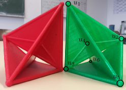
Figure 1: $K_{6}$ can be drawn straight-line and crossing-free on four planes. This is optimal, that is, $\rho^{2}_{3}(K_{6})=4$.

Figure 2: Planar 9-vertex graph $G$ with $\pi^{1}_{3}(G)=3$, 3D-drawing on three lines.

In a weaker setting, we require only the vertices to be located on a limited number of planes (or lines). For example, the graph in Fig. 2 can be drawn in 2D such that its vertices are contained in three lines; we conjecture that it is the smallest planar graph that needs more than two lines even in 3D. This version of our problem is related to the well-studied problem of drawing a graph straight-line in a 3D grid of bounded volume [17, 44]: If a graph can be drawn with all vertices on a grid of volume $v$, then $v^{1/3}$ planes and $v^{2/3}$ lines suffice. We now formalize the problem.

Definition 1

Let $1\leq l<d$, and let $G$ be a graph. We define the $l$-dimensional affine cover number of $G$ in $\mathbb{R}^{d}$, denoted by $\rho^{l}_{d}(G)$, as the minimum number of $l$-dimensional planes in $\mathbb{R}^{d}$ such that $G$ has a drawing that is contained in the union of these planes. We define $\pi^{l}_{d}(G)$, the weak $l$-dimensional affine cover number of $G$ in $\mathbb{R}^{d}$, similarly to $\rho^{l}_{d}(G)$, but under the weaker restriction that the vertices (and not necessarily the edges) of $G$ are contained in the union of the planes. Finally, the parallel affine cover number, $\bar{\pi}^{l}_{d}(G)$, is a restricted version of $\pi^{l}_{d}(G)$, in which we insist that the planes are parallel. We consider only straight-line and crossing-free drawings. Note: $\rho^{l}_{d}(G)$, $\pi^{l}_{d}(G)$, and $\bar{\pi}^{l}_{d}(G)$ are only undefined when $d=2$ and $G$ is non-planar.

Clearly, for any combination of $l$ and $d$, it holds that $\pi^{l}_{d}(G)\leq\bar{\pi}^{l}_{d}(G)$ and $\pi^{l}_{d}(G)\leq\rho^{l}_{d}(G)$. Larger values of $l$ and $d$ give us more freedom for drawing graphs and, therefore, smaller $\pi$- and $\rho$-values. Formally, for any graph $G$, if $l^{\prime}\leq l$ and $d^{\prime}\leq d$ then $\pi^{l}_{d}(G)\leq\pi^{l^{\prime}}_{d^{\prime}}(G)$, $\rho^{l}_{d}(G)\leq\rho^{l^{\prime}}_{d^{\prime}}(G)$, and $\bar{\pi}^{l}_{d}(G)\leq\bar{\pi}^{l^{\prime}}_{d^{\prime}}(G)$. But in most cases this freedom is not essential. For example, it suffices to consider $l\leq 2$ because otherwise $\rho^{l}_{d}(G)=1$. More interestingly, we can actually focus on $d\leq 3$ because every graph can be drawn in $3$-space as effectively as in high dimensional spaces, i.e., for any integers $1\leq l\leq d$, $d\geq 3$, and for any graph $G$, it holds that $\pi^{l}_{d}(G)=\pi^{l}_{3}(G)$, $\bar{\pi}^{l}_{d}(G)=\bar{\pi}^{l}_{3}(G)$, and $\rho^{l}_{d}(G)=\rho^{l}_{3}(G)$. We prove this important fact in Appendix 0.A. Thus, our task is to investigate the cases $1\leq l<d\leq 3$. We call $\rho^{1}_{2}(G)$ and $\rho^{1}_{3}(G)$ the line cover numbers in 2D and 3D, $\rho^{2}_{3}(G)$ the plane cover number, and analogously for the weak versions.

Related work.

We have already briefly mentioned 3D graph drawing on the grid, which has been surveyed by Wood [44] and by Dujmović and Whitesides [17]. For example, Dujmović [13], improving on a result of Di Battista et al. [4], showed that any planar graph can be drawn into a 3D-grid of volume $O(n\log n)$. It is well-known that, in 2D, any planar graph admits a plane straight-line drawing on an $O(n)\times O(n)$ grid [39, 22] and that the nested-triangles graph $T_{k}=K_{3}\times P_{k}$ (see Fig. 5, p. 5) with $3k$ vertices needs $\Omega(k^{2})$ area [22].

An interesting variant of our problem is to study drawings whose edge sets are represented (or covered) by as few objects as possible. The type of objects that have been used are straight-line segments [14, 19] and circular arcs [40]. The idea behind this objective is to keep the visual complexity of a drawing low for the observer. For example, Schulz [40] showed how to draw the dodecahedron by using $10$ arcs, which is optimal.

Our contribution.

Our research goes into three directions.

First, we show lower and upper bounds for the numbers of lines and planes needed for covering drawings of graphs in certain graph classes such as graphs of bounded degree or subclasses of planar graphs. The most natural graph families to start with are the complete graphs and the complete bipartite graphs. Most versions of the affine cover numbers of these graphs can be determined easily. Two cases are much more subtle: We determine $\rho^{2}_{3}(K_{n})$ and $\rho^{1}_{3}(K_{n,n})$ only asymptotically, up to a factor of 2 (see Theorem 2.4 and Example 2). Some efforts are made to compute the exact values of $\rho^{2}_{3}(K_{n})$ for small $n$ (see Theorem 2.5). As another result in this direction, we prove that $\rho^{1}_{3}(G)>n/5$ for almost all cubic graphs on $n$ vertices (Theorem 2.3(b)).

Second, we relate the affine cover numbers to standard combinatorial characteristics of graphs and to parameters that have been studied in graph drawing. In Section 2.1, we characterize $\pi^{1}_{3}(G)$ and $\pi^{2}_{3}(G)$ in terms of the linear vertex arboricity and the vertex thickness, respectively. This characterization implies that both $\pi^{1}_{3}(G)$ and $\pi^{2}_{3}(G)$ are linearly related to the chromatic number of the graph $G$. Along the way, we refine a result of Pach et al. [34] concerning the volume of 3D grid drawings (Theorem 2.1). We also prove that any graph $G$ has balanced separators of size at most $\rho^{1}_{3}(G)$ and conclude from this that $\rho^{1}_{3}(G)\geq\operatorname{tw}(G)/3$, where $\operatorname{tw}(G)$ denotes the treewidth of $G$ (Theorem 2.3). In Section 3.2, we analyze the relationship between $\rho^{1}_{2}(G)$ and the segment number $\operatorname{segm}(G)$ of a graph, which was introduced by Dujmović et al. [14]. We prove that $\operatorname{segm}(G)=O(\rho^{1}_{2}(G)^{2})$ for any connected $G$ and show that this bound is optimal (see Theorem 3.3 and Example 5).

Third, we pay special attention to planar graphs (Section 3). Among other results, we show examples of planar graphs with a large gap between the parameters $\rho^{1}_{3}(G)$ and $\rho^{1}_{2}(G)$ (see Theorem 3.4).

We also investigate the parallel affine cover numbers $\bar{\pi}^{1}_{2}$ and $\bar{\pi}^{1}_{3}$. Observe that for any graph $G$, $\bar{\pi}^{1}_{3}(G)$ equals the improper track number of $G$, which was introduced by Dujmović et al. [15].

Due to lack of space, our results for the parallel affine cover numbers (along with a survey of known related results) appear in Appendix 0.B. We defer some other proofs to Appendices 0.C and 0.D and list some open problems in Appendix 0.E.

Remark on the computational complexity.

In a follow-up paper [9], we investigate the computational complexity of computing the $\rho$- and $\pi$-numbers. We argue that it is NP-hard to decide whether a given graph has a $\pi^{1}_{3}$- or $\pi^{2}_{3}$-value of 2 and that both values are even hard to approximate. This result is based on Theorems 2.1 and 2.2 and Corollaries 1 and 2 in the present paper. While the graphs with $\rho_{3}^{2}$-value 1 are exactly the planar graphs (and hence, can be recognized in linear time), it turns out that recognizing graphs with a $\rho_{3}^{2}$-value of 2 is already NP-hard. In contrast to this, the problems of deciding whether $\rho^{1}_{3}(G)\leq k$ or $\rho^{1}_{2}(G)\leq k$ are solvable in polynomial time for any fixed $k$. However, the versions of these problems with $k$ being part of the input are complete for the complexity class $\exists\mathbb{R}$ which is based on the existential theory of the reals and that plays an important role in computational geometry [38].

Notation.

For a graph $G=(V,E)$, we use $n$ and $m$ to denote the numbers of vertices and edges of $G$, respectively. Let $\Delta(G)=\max_{v\in V}\deg(v)$ denote the maximum degree of $G$. Furthermore, we will use the standard notation $\chi(G)$ for the chromatic number, $\operatorname{tw}(G)$ for the treewidth, and $\operatorname{diam}(G)$ for the diameter of $G$. The Cartesian product of graphs $G$ and $H$ is denoted by $G\times H$.

2 The Affine Cover Numbers in $\mathbb{R}^{3}$

2.1 Placing Vertices on Few Lines or Planes ($\pi^{1}_{3}$ and $\pi^{2}_{3}$)

A linear forest is a forest whose connected components are paths. The linear vertex arboricity $\operatorname{lva}(G)$ of a graph $G$ equals the smallest size $r$ of a partition $V(G)=V_{1}\cup\dots\cup V_{r}$ such that every $V_{i}$ induces a linear forest. This notion, which is an induced version of the fruitful concept of linear arboricity (see Remark 1 below), appears very relevant to our topic. The following result is based on a construction of Pach et al. [34]; see Appendix 0.C for the proof.

Theorem 2.1

For any graph $G$, it holds that $\pi^{1}_{3}(G)=\operatorname{lva}(G)$. Moreover, any graph $G$ can be drawn with vertices on $r$ lines in the 3D integer grid of size $r\times 4rn\times 4r^{2}n$, where $r=\operatorname{lva}(G)$.

Corollary 1

$\chi(G)/2\leq\pi^{1}_{3}(G)\leq\chi(G)$.

Corollary 1 readily implies that $\pi^{1}_{3}(G)\leq\Delta(G)+1$ [7]. This can be considerably improved using a relationship between the linear vertex arboricity and the maximum degree that is established by Matsumoto [32]. Matsumoto’s result implies that $\pi^{1}_{3}(G)\leq\Delta(G)/2+1$ for any connected graph $G$. Moreover, if $\Delta(G)=2d$, then $\pi^{1}_{3}(G)=d+1$ if and only if $G$ is a cycle or the complete graph $K_{2d+1}$.

We now turn to the weak plane cover numbers. The vertex thickness $\operatorname{vt}(G)$ of a graph $G$ is the smallest size $r$ of a partition $V(G)=V_{1}\cup\dots\cup V_{r}$ such that $G[V_{1}],\dots,G[V_{r}]$ are all planar. We prove the following theorem in Appendix 0.C.

Theorem 2.2

For any graph $G$, it holds that $\pi^{2}_{3}(G)=\bar{\pi}^{2}_{3}(G)=\operatorname{vt}(G)$ and that $G$ can be drawn such that all vertices lie on a 3D integer grid of size $\operatorname{vt}(G)\times O(m^{2})\times O(m^{2})$, where $m$ is the number of edges of $G$. Note that this drawing occupies $\operatorname{vt}(G)$ planes.

Corollary 2

$\chi(G)/4\leq\pi^{2}_{3}(G)\leq\chi(G)$.

Example 1

1. $\pi^{1}_{3}(K_{n})=\lceil n/2\rceil$.

2. $\pi^{1}_{3}(K_{p,q})=2$ for any $1\leq p\leq q$; except for $\pi^{1}_{3}(K_{1,1})=\pi^{1}_{3}(K_{1,2})=1$.

3. $\pi^{2}_{3}(K_{n})=\lceil n/4\rceil$; therefore, $\pi^{2}_{3}(G)\leq\lceil n/4\rceil$ for every graph $G$.

2.2 Placing Edges on Few Lines or Planes ($\rho^{1}_{3}$ and $\rho^{2}_{3}$)

Clearly, $\Delta(G)/2\leq\rho^{1}_{3}(G)\leq m$ for any graph $G$. Call a vertex $v$ of a graph $G$ essential if $\deg v\geq 3$ or if $v$ belongs to a $K_{3}$ subgraph of $G$. Denote the number of essential vertices in $G$ by $\operatorname{es}(G)$.

Lemma 1

1. $\rho^{1}_{3}(G)>(1+\sqrt{1+8\operatorname{es}(G)})/2$.

2. $\rho^{1}_{3}(G)>\sqrt{m^{2}/n-m}$ for any graph $G$ with $m\geq n\geq 1$.

Proof

(a) In any drawing of a graph $G$, any essential vertex is shared by two edges not lying on the same line. Therefore, each such vertex is an intersection point of at least two lines, which implies that $\operatorname{es}(G)\leq\binom{\rho^{1}_{3}(G)}{2}$. Hence, $\rho^{1}_{3}(G)\geq\big{(}1+\sqrt{1+8\operatorname{es}(G)}\,\big{)}/2>\sqrt{2\operatorname{es}(G)}$.

(b) Taking into account multiplicity of intersection points (that is, each vertex $v$ requires at least $\lceil\deg v/2\rceil(\lceil\deg v/2\rceil-1)/2$ intersecting line pairs), we obtain

$$\binom{\rho^{1}_{3}(G)}{2} \geq \frac{1}{2}\sum_{v\in V(G)}\left\lceil\frac{\deg v}{2}\right\rceil\left(\left\lceil\frac{\deg v}{2}\right\rceil-1\right)\geq\sum\frac{\deg v(\deg v-2)}{8}=$$

$$= \frac{1}{8}\sum(\deg v)^{2}-\frac{1}{4}\sum\deg v\geq\frac{1}{8n}\left(\sum\deg v\right)^{2}-\frac{1}{4}2m=\frac{m^{2}}{2n}-\frac{m}{2}.$$

The last inequality follows by the inequality between arithmetic and quadratic means. Hence, $\rho^{1}_{3}(G)>\sqrt{m^{2}/n-m}$.

Part (a) of Lemma 1 implies that $\rho^{1}_{3}(G)>\sqrt{2n}$ if a graph $G$ has no vertices of degree 1 and 2, while Part (b) yields $\rho^{1}_{3}(G)>\sqrt{m/2}$ for all such $G$. Note that a disjoint union of $k$ cycles can have no essential vertices, but each cycle will need $3$ intersection points of lines, i.e., such a graph has $\rho^{1}_{3}\in\Omega(\sqrt{k})$. Thus, $\rho^{1}_{3}$ cannot be bounded from above by a function of essential vertices.

Remark 1

The linear arboricity $\operatorname{la}(G)$ of a graph $G$ is the minimum number of linear forests which partition the edge set of $G$; see [29]. Clearly, we have $\rho^{1}_{3}(G)\geq\operatorname{la}(G)$. There is no function of $\operatorname{la}(G)$ that is an upper bound for $\rho^{1}_{3}(G)$. Indeed, let $G$ be an arbitrary cubic graph. Akiyama et al. [2] showed that $\operatorname{la}(G)=2$. On the other hand, any vertex of $G$ is essential, so $\rho^{1}_{3}(G)>\sqrt{2n}$ by Lemma 1(a). Theorem 2.3 below shows an even larger gap.

We now prove a general lower bound for $\rho^{1}_{3}(G)$ in terms of the treewidth of $G$. Note for comparison that $\pi^{1}_{3}(G)\leq\chi(G)\leq\operatorname{tw}(G)+1$ (the last inequality holds because the graphs of treewidth at most $k$ are exactly partial $k$-trees and the construction of a $k$-tree easily implies that it is $k+1$-vertex-chromatic) . The relationship between $\rho^{1}_{3}(G)$ and $\operatorname{tw}(G)$ follows from the fact that graphs with low parameter $\rho^{1}_{3}(G)$ have small separators. This fact is interesting by itself and has yet another consequence: Graphs with bounded vertex degree can have linearly large value of $\rho^{1}_{3}(G)$ (hence, the factor of $n$ in the trivial bound $\rho^{1}_{3}(G)\leq m\leq\frac{1}{2}\,n\,\Delta(G)$ is best possible).

We need the following definitions. Let $W\subseteq V(G)$. A set of vertices $S\subset V(G)$ is a balanced $W$-separator of the graph $G$ if $|W\cap C|\leq|W|/2$ for every connected component $C$ of $G\setminus S$. Moreover, $S$ is a strongly balanced $W$-separator if there is a partition $W\setminus S=W_{1}\cup W_{2}$ such that $|W_{i}|\leq|W|/2$ for both $i=1,2$ and there is no path between $W_{1}$ and $W_{2}$ avoiding $S$. Let $\operatorname{sep}_{W}(G)$ (resp. $\operatorname{sep}^{*}_{W}(G)$) denote the minimum $k$ such that $G$ has a (resp. strongly) balanced $W$-separator $S$ with $|S|=k$. Furthermore, let $\operatorname{sep}(G)=\operatorname{sep}_{V(G)}(G)$ and $\operatorname{sep}^{*}(G)=\operatorname{sep}^{*}_{V(G)}(G)$. Note that $\operatorname{sep}_{W}(G)\leq\operatorname{sep}^{*}_{W}(G)$ for any $W$ and, in particular, $\operatorname{sep}(G)\leq\operatorname{sep}^{*}(G)$.

It is known [21, Theorem 11.17] that $\operatorname{sep}_{W}(G)\leq\operatorname{tw}(G)+1$ for every $W\subseteq V(G)$. On the other hand, if $\operatorname{sep}_{W}(G)\leq k$ for all $W$ with $|W|=2k+1$, then $\operatorname{tw}(G)\leq 3k$.

The bisection width $\operatorname{bw}(G)$ of a graph $G$ is the minimum possible number of edges between two sets of vertices $W_{1}$ and $W_{2}$ with $|W_{1}|=\lceil n/2\rceil$ and $|W_{2}|=\lfloor n/2\rfloor$ partitioning $V(G)$. Note that $\operatorname{sep}^{*}(G)\leq\operatorname{bw}(G)+1$.

Theorem 2.3

1. $\rho^{1}_{3}(G)\geq\operatorname{bw}(G)$.

2. $\rho^{1}_{3}(G)>n/5$ for almost all cubic graphs with $n$ vertices.

3. $\rho^{1}_{3}(G)\geq\operatorname{sep}^{*}_{W}(G)$ for every $W\subseteq V(G)$.

4. $\rho^{1}_{3}(G)\geq\operatorname{tw}(G)/3$.

Proof

(a) Fix a drawing of the graph $G$ on $r=\rho^{1}_{3}(G)$ lines in $\mathbb{R}^{3}$. Choose a plane $L$ that is not parallel to any of the at most $\binom{n}{2}$ lines passing through two vertices of the drawing. Let us move $L$ along the orthogonal direction until it separates the vertex set of $G$ into two almost equal parts $W_{1}$ and $W_{2}$. The plane $L$ can intersect at most $r$ edges of $G$, which implies that $\operatorname{bw}(G)\leq r$.

(b) follows from Part (a) and the fact that a random cubic graph on $n$ vertices has bisection width at least $n/4.95$ with probability $1-o(1)$ (Kostochka and Melnikov [30]).

(c) Given $W\subseteq V(G)$, we have to prove that $\operatorname{sep}^{*}_{W}(G)\leq\rho^{1}_{3}(G)$. Choose a plane $L$ as in the proof of Part (a) and move it until it separates $W$ into two equal parts $W^{\prime}_{1}$ and $W^{\prime}_{2}$; if $|W|$ is odd, then $L$ should contain one vertex $w$ of $W$. If $|W|$ is even, we can ensure that $L$ does not contain any vertex of $G$. We now construct a set $S$ as follows. If $L$ contains a vertex $w\in W$, i.e., $|W|$ is odd, we put $w$ in $S$. Let $E$ be the set of those edges which are intersected by $L$ but are not incident to the vertex $w$ (if it exists). Note that $|E|<r$ if $|W|$ is odd and $|E|\leq r$ if $|W|$ is even. Each of the edges in $E$ contributes one of its incident vertices into $S$. Note that $|S|\leq r$. Set $W_{1}=W^{\prime}_{1}\setminus S$ and $W_{2}=W^{\prime}_{2}\setminus S$ and note that there is no edge between these sets of vertices. Thus, $S$ is a strongly balanced $W$-separator.

(d) follows from (c) by the relationship between treewidth and balanced separators.

On the other hand, note that $\rho^{1}_{3}(G)$ cannot be bounded from above by any function of $\operatorname{tw}(G)$. Indeed, by Lemma 1(a) we have $\rho^{1}_{3}(T)=\Omega(\sqrt{n})$ for every caterpillar $T$ with linearly many vertices of degree 3. The best possible relation in this direction is $\rho^{1}_{3}(G)\leq m<n\operatorname{tw}(G)$. The factor $n$ cannot be improved here (take $G=K_{n}$).

Example 2

1. $\rho^{1}_{3}(K_{n})=\binom{n}{2}$ for any $n\geq 2$.

2. $pq/2\leq\rho^{1}_{3}(K_{p,q})\leq pq$ for any $1\leq p\leq q$.

We now turn to the plane cover number.

Example 3

For any integers $1\leq p\leq q$, it holds that $\rho^{2}_{3}(K_{p,q})=\lceil p/2\rceil$.

Determining the parameter $\rho^{2}_{3}(G)$ for complete graphs $G=K_{n}$ is a much more subtle issue. We are able to determine the asymptotics of $\rho^{2}_{3}(K_{n})$ up to a factor of 2.

By a combinatorial cover of a graph $G$ we mean a set of subgraphs $\{G_{i}\}$ such that every edge of $G$ belongs to $G_{i}$ for some $i$. A geometric cover of a crossing-free drawing $d\colon V(K_{n})\to\mathbb{R}^{3}$ of a complete graph $K_{n}$ is a set $\mathcal{L}$ of planes in $\mathbb{R}^{3}$ so that for each pair of vertices $v_{i},v_{j}\in V(K_{n})$ there is a plane $\ell\in\mathcal{L}$ containing both points $d(v_{i})$ and $d(v_{j})$. This geometric cover $\mathcal{L}$ induces a combinatorial cover $\mathcal{K}_{\mathcal{L}}=\{G_{\ell}\mid\ell\in\mathcal{L}\}$ of the graph $K_{n}$, where $G_{\ell}$ is the subgraph of $K_{n}$ induced by the set $d^{-1}(\ell)$. Note that each $G_{\ell}$ is a $K_{s}$ subgraph with $s\leq 4$ (because $K_{5}$ is not planar).

Let $c(K_{n},K_{s})$ denote the minimum size of a combinatorial cover of $K_{n}$ by $K_{s}$ subgraphs ($c(K_{n},K_{s})=0$ if $s>n$). The asymptotics of the numbers $c(K_{n},K_{s})$ for $s=3,4$ can be determined via the results about Steiner systems by Kirkman and Hanani [5, 28]. This yields the following bounds for $\rho^{2}_{3}(K_{n})$ (see Appendix 0.C).

Theorem 2.4

For all $n\geq 3$,

$$\left(1/2+o(1)\right)n^{2}=c(K_{n},K_{4})\leq\rho^{2}_{3}(K_{n})\leq c(K_{n},K_{3})=\left(1/6+o(1)\right)n^{2}.$$

Note that we cannot always realize a combinatorial cover of $K_{n}$ by copies of $K_{4}$ geometrically. For example, $c(K_{6},K_{4})=3<4=\rho^{2}_{3}(K_{6})$ (see Theorem 2.5).

In order to determine $\rho^{2}_{3}(K_{n})$ for particular values of $n$, we need some properties of geometric and combinatorial covers of $K_{n}$.

Lemma 2

Let $d\colon V(K_{n})\to\mathbb{R}^{3}$ be a crossing-free drawing of $K_{n}$ and $\mathcal{L}$ a geometric cover of $d$. For each 4-vertex graph $G_{\ell}\in\mathcal{K}_{\mathcal{L}}$, the set $d(G_{\ell})$ not only belongs to a plane $\ell$, but also defines a triangle with an additional vertex in its interior.

Lemma 3

Let $d\colon V(K_{n})\to\mathbb{R}^{3}$ be a crossing-free drawing of $K_{n}$ and $\mathcal{L}$ a geometric cover of $d$. No two different 4-vertex graphs $G_{\ell},G_{\ell^{\prime}}\in\mathcal{K}_{\mathcal{L}}$ can have three common vertices.

Theorem 2.5

For $n\leq 9$, the value of $\rho^{2}_{3}(K_{n})$ is bounded by the numbers in Table 1.

Table 1: Lower and upper bounds for $\rho^{2}_{3}(K_{n})$ for small values of $n$.

$n$	4	5	6	7	8	9
$\geq$	1	3	4	6	6	7
$\leq$	1	3	4	6	7

Proof

Here, we show only the bounds for $n=6$. For the remaining proofs, see Appendix 0.C. Fig. 2 shows that $\rho^{2}_{3}(K_{6})\leq 4$. Now we show that $\rho^{2}_{3}(K_{6})\geq 4$. Assume that $\rho^{2}_{3}(K_{6})<4$. Consider a combinatorial cover $\mathcal{K}_{\mathcal{L}}$ of $K_{6}$ by its complete planar subgraphs corresponding to a geometric cover $\mathcal{L}$ of its drawing by $3$ planes. Graph $K_{6}$ has $15$ edges, so to cover it by complete planar graphs we have to use at least two copies of $K_{4}$ and, additionally, a copy of $K_{k}$ for $3\leq k\leq 4$. But, since each two copies of $K_{4}$ in $K_{6}$ have a common edge (and by Lemma 3 this edge is unique), the cover $\mathcal{K}_{\mathcal{L}}$ consists of three copies of $K_{4}$. Denote these copies by $K_{4}^{1}$, $K_{4}^{2}$, and $K_{4}^{3}$. By Lemma 2, for each $i$, $d(K_{4}^{i})$ is a triangle with an additional vertex $d(v_{i})$ in its interior. Let $V_{0}=\{v_{1},v_{2},v_{3}\}$. By the Krein–Milman theorem [31, 42], the convex hull $\operatorname{Conv}(d(K_{6}))$ is the convex hull $\operatorname{Conv}(d(V(K_{6}))\setminus d(V_{0}))$. If all the vertices $v_{i}$ are mutually distinct then the set $d(V(K_{6}))\setminus d(V_{0})$ is a triangle, so the drawing $d$ is planar, a contradiction. Hence, $v_{i}=v_{j}$ for some $i\neq j$. Let $k$ be the third index that is distinct from both $i$ and $j$. Since graphs $K_{4}^{i}$ and $K_{4}^{j}$ have exactly one common edge, this is an edge $(v_{i},v)$ for some vertex $v$ of $K_{6}$ (see Fig. 2 with $u_{4}$ for $v_{i}$ and $u_{1}$ for $v$). Let $V(K_{4}^{i})=\{v,v_{i},v_{i}^{1},v_{i}^{2}\}$ and $V(K_{4}^{j})=\{v,v_{j},v_{j}^{1},v_{j}^{2}\}$. Since the union $K_{4}^{1}\cup K_{4}^{2}\cup K_{4}^{3}$ covers all edges of $K_{6}$, all edges $(v_{i}^{1},v_{j}^{1})$, $(v_{i}^{1},v_{j}^{2})$, $(v_{i}^{2},v_{j}^{1})$, and $(v_{i}^{2},v_{j}^{2})$ belong to $K_{4}^{k}$. Thus $V(K_{4}^{k})=\{v_{i}^{1},v_{i}^{2},v_{j}^{1},v_{j}^{2}\}$. But vertices $v_{i}^{1}$, $v_{i}^{2}$, $v_{j}^{1}$, and $v_{j}^{2}$ are in convex position (see Fig. 2), a contradiction to Lemma 2.

3 The Affine Cover Numbers of Planar Graphs ($\mathbb{R}^{2}$ and $\mathbb{R}^{3}$)

3.1 Placing Vertices on Few Lines ($\pi^{1}_{2}$ and $\pi^{1}_{3}$)

Combining Corollary 1 with the 4-color theorem yields $\pi^{1}_{3}(G)\leq 4$ for planar graphs. Given that outerplanar graphs are 3-colorable (they are partial 2-trees), we obtain $\pi^{1}_{3}(G)\leq 3$ for these graphs. These bounds can be improved using the equality $\pi^{1}_{3}(G)=\operatorname{lva}(G)$ of Theorem 2.1 and known results on the linear vertex arboricity:

1. For any planar graph $G$, it holds that $\pi^{1}_{3}(G)\leq 3$ [24, 35].

2. There is a planar graph $G$ with $\pi^{1}_{3}(G)=3$ [10].

3. For any outerplanar graph $G$, $\pi^{1}_{3}(G)\leq 2$ [1, 6, 41].

According to Chen and He [11], the upper bound $\operatorname{lva}(G)\leq 3$ for planar graphs by Poh [35] is constructive and yields a polynomial-time algorithm for partitioning the vertex set of a given planar graph into three parts, each inducing a linear forest. By combining this with the construction given in Theorem 2.1, we obtain a polynomial-time algorithm that draws a given planar graph such that the vertex set “sits” on three lines.

The example of Chartrand and Kronk [10] is a 21-vertex planar graph whose vertex arboricity is 3, which means that the vertex set of this graph cannot even be split into two parts both inducing (not necessarily linear) forests. Raspaud and Wang [36] showed that all 20-vertex planar graphs have vertex arboricity at most 2. We now observe that a smaller example of a planar graph attaining the extremal value $\pi^{1}_{3}(G)=3$ can be found by examining the linear vertex arboricity.

Example 4

The planar 9-vertex graph $G$ in Fig. 2 has $\pi^{1}_{3}(G)=\operatorname{lva}(G)=3$. (See a proof in Appendix 0.D.)

Now we show lower bounds for the parameter $\pi^{1}_{2}(G)$.

Recall that the circumference of a graph $G$, denoted by $c(G)$, is the length of a longest cycle in $G$. For a planar graph $G$, let $\bar{v}(G)$ denote the maximum $k$ such that $G$ has a straight-line plane drawing with $k$ collinear vertices.

Lemma 4

Let $G$ be a planar graph. Then $\pi^{1}_{2}(G)\geq n/\bar{v}(G)$. If $G$ is a triangulation then $\pi^{1}_{2}(G)\geq(2n-4)/c(G^{*})$.

Proof

Since the first claim is obvious, we prove only the second. Let $\gamma(G)$ denote the minimum number of cycles in the dual graph $G^{*}$ sharing a common vertex and covering every vertex of $G^{*}$ at least twice. Note that, as $G$ is a triangulation, $\gamma(G)\geq(4n-8)/c(G^{*})$, where $2n-4$ is the number of vertices in $G^{*}$ (as a consequence of Euler’s formula). We now show $\pi^{1}_{2}(G)\geq\gamma(G)/2$, which implies the claimed result.

Given a drawing realizing $\pi^{1}_{2}(G)$ with line set $\mathcal{L}$, for every line $\ell\in\mathcal{L}$, draw two parallel lines $\ell^{\prime},\ell^{\prime\prime}$ sufficiently close to $\ell$ such that they together intersect the interiors of all faces touched by $\ell$ and do not go through any vertex of the drawing. Note that $\ell^{\prime}$ and $\ell^{\prime\prime}$ cross boundaries of faces only via inner points of edges. Each such crossing corresponds to a transition from one vertex to another along an edge in the dual graph $G^{*}$. Since all the faces of $G$ are triangles, each of them is visited by each of $\ell^{\prime}$ and $\ell^{\prime\prime}$ at most once. Therefore, the faces crossed along $\ell^{\prime}$ and the faces crossed along $\ell^{\prime\prime}$, among them the outer face of $G$, each form a cycle in $G^{*}$. It remains to note that every face $f$ of the graph $G$ is crossed at least twice, because $f$ is intersected by at least two different lines from $\mathcal{L}$ and each of these two lines has a parallel copy that crosses $f$.

An infinite family of triangulations $G$ with $\bar{v}(G)\leq n^{0.99}$ is constructed in [37]. By the first part Lemma 4 this implies that there are infinitely many triangulations $G$ with $\pi^{1}_{2}(G)\geq n^{0.01}$. The second part of Lemma 4 along with an estimate of Grünbaum and Walther [26] (that was used also in [37]) yields a stronger result.

Theorem 3.1

There are infinitely many triangulations $G$ with $\Delta(G)\leq 12$ and $\pi^{1}_{2}(G)\geq n^{0.01}$.

Proof

The shortness exponent $\sigma_{\mathcal{G}}$ of a class $\mathcal{G}$ of graphs is the infimum of the set of the reals $\liminf_{i\to\infty}{\log c(H_{i})}/{\log|V(H_{i})|}$ for all sequences of $H_{i}\in\mathcal{G}$ such that $|V(H_{i})|<|V(H_{i+1})|$. Thus, for each $\epsilon>0$, there are infinitely many graphs $H\in\mathcal{G}$ with $c(H)<|V(H)|^{\sigma_{\mathcal{G}}+\epsilon}$. The dual graphs of triangulations with maximum vertex degree at most 12 are exactly the cubic 3-connected planar graphs with each face incident to at most 12 edges (this parameter is well defined by the Whitney theorem). Let $\sigma$ denote the shortness exponent for this class of graphs. It is known [26] that $\sigma\leq\frac{\log 26}{\log 27}=0.988\ldots$. The theorem follows from this bound by the second part of Lemma 4.

Problem 1

Does $\pi^{1}_{2}(G)=o(n)$ hold for all planar graphs $G$?

A track drawing [20] of a graph is a plane drawing for which there are parallel lines, called tracks, such that every edge either lies on a track or its endpoints lie on two consecutive tracks. We call a graph track drawable if it has a track drawing. Let $\operatorname{tn}(G)$ be the minimum number of tracks of a track drawing of $G$. Note that $\pi^{1}_{2}(G)\leq\bar{\pi}^{1}_{2}(G)\leq\operatorname{tn}(G)$.

The following proposition is similar to a lemma of Bannister et al. [3, Lemma 1] who say it is implicit in the earlier work of Felsner et al. [20].

Theorem 3.2 (cf. [20, 3])

Let $G$ be a track drawable graph. Then $\pi^{1}_{2}(G)\leq 2$.

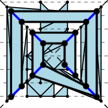
Figure 8: Proof of Theorem 3.2

Proof. Consider a track drawing of $G$, which we now transform to a drawing on two intersecting lines. Put the tracks consecutively along a spiral so that they correspond to disjoint intervals on the half-lines as depicted on the right. Tracks whose indices are equal modulo 4 are placed on the same half-line; for more details see Fig. 8 in Appendix 0.D on page 8. (Bannister et al. [3, Fig. 1] use three half-lines meeting in a point.) ∎

Observe that any tree is track drawable: two vertices are aligned on the same track iff they are at the same distance from an arbitrarily assigned root. Moreover, any outerplanar graph is track drawable [20]. This yields an improvement over the bound $\pi^{1}_{3}(G)\leq 2$ for outerplanar graphs stated in the beginning of this section.

Corollary 3

For any outerplanar graph $G$, it holds that $\pi^{1}_{2}(G)\leq 2$.

3.2 Placing Edges on Few Lines ($\rho^{1}_{2}$ and $\rho^{1}_{3}$)

The parameter $\rho^{1}_{2}(G)$ is related to two parameters introduced by Dujmović et al. [14]. They define a segment in a straight-line drawing of a graph $G$ as an inclusion-maximal (connected) path of edges of $G$ lying on a line. A slope is an inclusion-maximal set of parallel segments. The segment number (resp., slope number) of a planar graph $G$ is the minimum possible number of segments (resp., slopes) in a straight-line drawing of $G$. We denote these parameters by $\operatorname{segm}(G)$ (resp., $\operatorname{slop}(G)$). Note that $\operatorname{slop}(G)\leq\rho^{1}_{2}(G)\leq\operatorname{segm}(G)$.

These parameters can be far away from each other. Figure 5 shows a graph with $\operatorname{slop}(G)=O(1)$ and $\rho^{1}_{2}(G)=\Omega(n)$ (see the proof of Theorem 3.4). On the other hand, note that $\rho^{1}_{2}(mK_{2})=1$ while $\operatorname{segm}(mK_{2})=m$ where $mK_{2}$ denotes the graph consisting of $m$ isolated edges. The gap between $\rho^{1}_{2}(G)$ and $\operatorname{segm}(G)$ can be large even for connected graphs. It is not hard to see that $\operatorname{segm}(G)$ is bounded from below by half the number of odd degree vertices (see [14] for details). Therefore, if we take a caterpillar $G$ with $k$ vertices of degree 3 and $k+2$ leaves, then $\operatorname{segm}(G)\geq n/2$, while $\rho^{1}_{2}(G)=O(\sqrt{n})$ because $G$ can easily be drawn in a square grid of area $O(n)$. Note that, for the same $G$, the gap between $\operatorname{slop}(G)$ and $\rho^{1}_{2}(G)$ is also large. Indeed, $\operatorname{slop}(G)=2$ while $\rho^{1}_{2}(G)>\sqrt{n-2}$ by Lemma 1(a).

It turns out that a large gap between $\rho^{1}_{2}(G)$ and $\operatorname{segm}(G)$ can be shown also for 3-connected planar graphs and even for triangulations.

Example 5

There are triangulations with $\rho^{1}_{2}(G)=O(\sqrt{n})$ and $\operatorname{segm}(G)=\Omega(n)$. Note that this gap is the best possible because any 3-connected graph $G$ has minimum vertex degree $3$ and, hence, $\rho^{1}_{2}(G)\geq\rho^{1}_{3}(G)>\sqrt{2n}$ by Lemma 1(a). Consider the graph shown in Fig. 5. Its vertices are placed on the standard orthogonal grid and two slanted grids, which implies that at most $O(\sqrt{n})$ lines are involved. The pattern can be completed to a triangulation by adding three vertices around it and connecting them to the vertices on the pattern boundary. Since the pattern boundary contains $O(\sqrt{n})$ vertices, $O(\sqrt{n})$ new lines suffice for this. Thus, we have $\rho^{1}_{2}(G)=O(\sqrt{n})$ for the resulting triangulation $G$. Note that the vertices drawn fat in Fig. 5 have degree $5$, and there are linearly many of them. This implies that $\operatorname{segm}(G)=\Omega(n)$.

Figure 3: The main body of a triangulation $G$ with $\rho^{1}_{2}(G)=O(\sqrt{n})$ and $\operatorname{segm}(G)=\Omega(n)$.

Figure 4: The nested-triangles graph $T_{k}$.

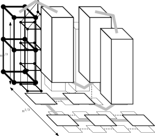
Figure 5: Sketch of the construction in the proof of Theorem 3.4(b).

Somewhat surprisingly, the parameter $\operatorname{segm}(G)$ can be bounded from above by a function of $\rho^{1}_{2}(G)$ for all connected graphs.

Theorem 3.3

For any connected planar graph $G$, $\operatorname{segm}(G)=O(\rho^{1}_{2}(G)^{2})$.

Note that $\Delta(G)/2\leq\rho^{1}_{3}(G)\leq\rho^{1}_{2}(G)\leq\operatorname{segm}(G)\leq m$ for any planar graph $G$. For all inequalities here except the second one, we already know that the gap between the respective pair of parameters can be very large (by considering a caterpillar with linearly many degree 3 vertices and applying Lemma 1(a), by Example 5, and by considering the path graph $P_{n}$, for which $\operatorname{segm}(P_{n})=1$). Part (b) of the following theorem shows a large gap also between the parameters $\rho^{1}_{3}(G)$ and $\rho^{1}_{2}(G)$, that is, some planar graphs can be drawn much more efficiently, with respect to the line cover number, in 3-space than in the plane.

Theorem 3.4

1. There are infinitely many planar graphs with constant maximum degree, constant treewidth, and linear $\rho^{1}_{2}$-value.

2. For infinitely many $n$ there is a planar graph $G$ on $n$ vertices with $\rho^{1}_{2}(G)=\Omega(n)$ and $\rho^{1}_{3}(G)=O(n^{2/3})$.

Proof

Consider the nested-triangles graph $T_{k}=C_{3}\times P_{k}$ shown in Fig. 5. To prove statements (a) and (b), it suffices to establish the following bounds:

1. $\rho^{1}_{2}(T_{k})\geq n/2$ and

2. $\rho^{1}_{3}(T_{k})=O(n^{2/3})$.

To see the linear lower bound (i), note that $T_{k}$ is 3-connected. Hence, Whitney’s theorem implies that, in any plane drawing of $T_{k}$, there is a sequence of nested triangles of length at least $k/2$. The sides of the triangles in this sequence must belong to pairwise different lines. Therefore, $\rho^{1}_{2}(T_{k})\geq 3k/2=n/2$.

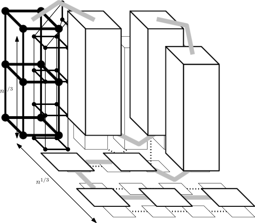
Figure 11: The graph $C_{4}\times P_{k}$ drawn into a 3D grid of linear volume on $O(n^{2/3})$ lines (the proof of Theorem 3.4(b)).

For the sublinear upper bound (ii), first consider the graph $C_{4}\times P_{k}$. We build wireframe rectangular prisms that are stacks of $O(\sqrt[3]{n})$ squares each. These prisms are placed onto the base plane in an $O(\sqrt[3]{n})\times O(\sqrt[3]{n})$ grid; see Fig. 5. So far we can place the edges on the $O(n^{2/3})$ lines of the 3D cubic grid of volume $O(n)$. Next, we construct a path that traverses all squares by passing through the prisms from top to bottom (resp., vice versa) and connecting neighboring prims. We rotate and move some of the squares at the top (resp., bottom) of the prisms to be able to draw the edges between neighboring prisms according to this path. For this “bending” we need $O(n^{2/3})$ additional lines. In Appendix 0.D we provide a drawing; see Fig. 11 on page 11. The same approach works for the graph $T_{k}=C_{3}\times P_{k}$. In addition to the standard 3D grid, here we need also its slanted, diagonal version (and, again, additional lines for bending in the cubic box of volume $O(n)$). The number of lines increases just by a constant factor.

We are able to determine the exact values of $\rho^{1}_{2}(G)$ for complete bipartite graphs $K_{p,q}$ that are planar.

Example 6

$\rho^{1}_{2}(K_{1,q})=\lceil m/2\rceil$ and $\rho^{1}_{2}(K_{2,q})=\lceil(3n-7)/2\rceil=\lceil(3m-2)/4\rceil$. See Appendix 0.D for details.

Motivated by Example 6, we ask:

Problem 2

What is the smallest $c$ such that $\rho^{1}_{2}(G)\leq(c+o(1))m$ for any planar graph $G$? Example 6 shows that $c\geq 3/4$. Durocher and Mondal [19], improving on an earlier bound of Dujmović et al. [14], showed that $\operatorname{segm}(G)<\frac{7}{3}n$ for any planar graph $G$. This implies that $c\leq 7/9$.

For any binary tree $T$, it holds that $\rho^{1}_{2}(T)=O(\sqrt{n\log n})$. This follows from the known fact [8] that $T$ has an orthogonal drawing on a grid of size $O(\sqrt{n\log n})\times O(\sqrt{n\log n})$. For complete binary trees lower and upper bounds are described in Example 13 in Appendix 0.D.

Appendix

Appendix 0.A Collapse of the Multidimensional Affine Hierarchy

Theorem 0.A.1

For any integers $1\leq l\leq d$, $d\geq 3$, and for any graph $G$, it holds that $\pi^{l}_{d}(G)=\pi^{l}_{3}(G)$, $\bar{\pi}^{l}_{d}(G)=\bar{\pi}^{l}_{3}(G)$, and $\rho^{l}_{d}(G)=\rho^{l}_{3}(G)$.

Proof

The theorem follows from the following fact: For any finite family $\mathcal{L}$ of lines in $\mathbb{R}^{d}$, there exists a linear transformation $A\colon\mathbb{R}^{d}\to\mathbb{R}^{3}$ that is injective on $L_{0}=\bigcup\left\{\hskip 1.42262pt\ell:\hskip 1.42262pt\ell\in\mathcal{L}\right\}$, the set of all points of the lines in $\mathcal{L}$.

We prove this claim by induction on $d$. If $d=3$, we let $A$ be the identity map on $\mathbb{R}^{3}$. Suppose that $d>3$.

Regarding two lines $\ell$ and $\ell^{\prime}$ in $\mathbb{R}^{d}$ as 1-dimensional affine subspaces, we consider the Minkowski difference $\ell-\ell^{\prime}=\left\{\hskip 1.42262ptl-l^{\prime}:\hskip 1.42262ptl\in\ell,\,l^{\prime}\in\ell^{\prime}\right\}$. Note that this is a plane, i.e., a 2-dimensional affine subspace of $\mathbb{R}^{d}$. Denote $L=L_{0}-L_{0}=\bigcup\left\{\hskip 1.42262pt\ell-\ell^{\prime}:\hskip 1.42262pt\ell,\ell^{\prime}\in\mathcal{L}\right\}$. Let $L^{\prime}=\left\{\hskip 1.42262pttl:\hskip 1.42262ptt\in\mathbb{R},\,l\in L\right\}$ be the union of all lines going through the origin $0$ of $\mathbb{R}^{d}$ and intersecting the set $L$. Since the set $L$ is contained in a union of finitely many planes in the space $\mathbb{R}^{d}$, the set $L^{\prime}$ is contained in a union of finitely many $3$-dimensional linear subspaces of $\mathbb{R}^{d}$ (each of them contains the origin $0$). Since $d>3$, there exists a line $\ell_{0}\ni 0$ such that $\ell_{0}\cap L=\{0\}$. Now, let $A_{0}:\mathbb{R}^{d}\rightarrow\mathbb{R}^{d-1}$ be an arbitrary linear transformation such that $\ker A_{0}=\ell_{0}$. Let $x,y\in L_{0}$ be arbitrary points such that $A_{0}x=A_{0}y$. Then $x-y\in(L_{0}-L_{0})\cap\ker A_{0}=L\cap\ell_{0}=\{0\}$, so $x=y$. Thus, the map $A_{0}$ is injective on $L_{0}$.

By the inductive assumption applied to the family of lines $\left\{\hskip 1.42262ptA_{0}\ell:\hskip 1.42262pt\ell\in\mathcal{L}\right\}$ in $\mathbb{R}^{d-1}$, there exists a linear transformation $A_{1}:\mathbb{R}^{d-1}\rightarrow\mathbb{R}^{3}$ injective on the union of all $\ell\in\mathcal{L}$. It remains to take the composition $A=A_{1}A_{0}$.

Appendix 0.B The Parallel Affine Cover Numbers

0.B.1 Placing Vertices on Few Parallel Lines in 3-Space ($\bar{\pi}^{1}_{3}$)

The concept of a proper track drawing was introduced by Dujmović et al. [16] in combinatorial terms with the following geometric meaning. We call a 3D drawing of a graph $G$ a proper track drawing if there are parallel lines, called tracks, such that every vertex of $G$ lies on one of the tracks and every edge connects vertices lying on two different tracks. Edges between any two tracks are not allowed to cross each other. Furthermore, we call a drawing of $G$ an improper track drawing if we allow edges between consecutive vertices of a same track. The proper track number $\operatorname{tn}^{\mathrm{p}}(G)$ (improper track number $\operatorname{tn}^{\mathrm{i}}(G)$) of $G$ is the minimum number of tracks of a proper (improper) track drawing of $G$. While the definition above does not excludes crossing of two edges if they are between disjoint pairs of tracks, note that all such crossings can be removed by slightly shifting the vertices within each track. We, therefore, have

$$\bar{\pi}^{1}_{3}(G)=\operatorname{tn}^{\mathrm{i}}(G)$$

for any graph $G$. By [15, Lemma 2.2], $\operatorname{tn}^{\mathrm{p}}(G)/2\leq\operatorname{tn}^{\mathrm{i}}(G)\leq\operatorname{tn}^{\mathrm{p}}(G)$. Therefore, the upper bounds for $\operatorname{tn}^{\mathrm{p}}(G)$ surveyed by Dujmović et al. [16, Table 1]) imply also upper bounds on $\bar{\pi}^{1}_{3}(G)$ for different classes of graphs $G$.

In particular, Dujmović, Morin, and Wood [15] prove that

$$\operatorname{tn}^{\mathrm{p}}(G)\leq 3^{\operatorname{tw}(G)}\cdot 6^{(4^{\operatorname{tw}(G)}-3{\operatorname{tw}(G)}-1)/9}$$

for any graph $G$. Note that any upper bound for $\bar{\pi}^{1}_{3}(G)$ implies also an upper bound for $\rho^{2}_{3}(G)$.

Lemma 5

$\rho^{2}_{3}(G)\leq\binom{\bar{\pi}^{1}_{3}(G)}{2}$.

Proof

Any two parallel lines of the drawing lie in a plane, and all the edges are located in these planes.

Since $\bar{\pi}^{1}_{3}(G)\leq\operatorname{tn}^{\mathrm{p}}(G)$, Lemma 5 implies that the parameter $\rho^{2}_{3}(G)$ is bounded from above by a function of the treewidth of $G$.

Whether or not $\operatorname{tn}^{\mathrm{p}}(G)$ and, hence, $\bar{\pi}^{1}_{3}(G)$ is bounded for the class of planar graphs is a long-standing open problem; see [15]. The best lower bound is $\bar{\pi}^{1}_{3}(G)\geq 7$; see [16, Cor. 10]. The best upper bound $\bar{\pi}^{1}_{3}(G)=O(\sqrt{n})$ for planar graphs is obtained by Dujmović and Wood [18]. Wood [43, Theorem 2] proved that for all $\Delta\geq 3$ and for all sufficiently large $n>n(\Delta)$, there is a simple $\Delta$-regular $n$-vertex graph with $\operatorname{tn}^{\mathrm{p}}(G)\geq c\sqrt{\Delta}n^{1/2-1/\Delta}$ for some absolute constant $c$, which implies that $\bar{\pi}^{1}_{3}(G)$ is unbounded even over graphs of bounded degree.

Theorem 0.B.1

1. If $\bar{\pi}^{1}_{3}(G)\leq 3$ then $G$ is planar and $\pi^{1}_{2}(G)\leq\bar{\pi}^{1}_{3}(G)$.

2. If $\pi^{1}_{2}(G)\leq 2$ for a planar graph $G$, then $\bar{\pi}^{1}_{3}(G)\leq 4$.

3. If $G$ is, moreover, track drawable, then $\bar{\pi}^{1}_{3}(G)\leq 3$.

Proof

(a) Since any two parallel lines in $\mathbb{R}^{3}$ define a plane, the graph $G$ can be drawn on the three rectangular faces of a triangular prism in $\mathbb{R}^{3}$, created by (a projection of) the parallel lines. Therefore, $G$ is planar. Now pick a point outside of the prism, but close to its triangular base. Project the drawing of $G$ on a plane that does not intersect the prism, is close and parallel to the other triangular face of the prism. This yields a drawing of $G$ whose vertices lie on $\bar{\pi}^{1}_{3}(G)$ lines.

(b) Assume that the graph $G$ is drawn on two lines $\ell_{1}$ and $\ell_{2}$. If these lines are parallel then $\bar{\pi}^{1}_{3}(G)\leq\bar{\pi}^{1}_{2}(G)\leq 2$ and we are done. If the lines $\ell_{1}$ and $\ell_{2}$ intersect in a point $O$, then the union $\ell_{1}\cup\ell_{2}$ is split into three open rays and one half-open ray. We can put the vertices from the rays into four parallel tracks, preserving their order from the point $O$ to infinity along the rays.

(c) This part is a version of Theorem 3.2.

Example 7

The parallel affine cover number of complete (bipartite) graphs is as follows.

1. $\bar{\pi}^{1}_{3}(K_{n})=n-1$ for any $n\geq 2$.

2. $\bar{\pi}^{1}_{3}(K_{p,q})=p+1$ for any $p\leq q$ and $q\geq 3$.

Part (a) is straightforward.

Let us prove Part (b) (for the proper track number the case $p=q$ was considered by Dujmović and Whitesides [17]) To show the upper bound $\bar{\pi}^{1}_{3}(K_{p,q})\leq p+1$, we put the independent set of $q$ vertices in a line and use a separate line for each of the other $p$ vertices. To show the lower bound, let $\mathcal{L}$ be an optimal set of lines. Suppose that our bipartition is defined by $p$ white and $q$ black vertices. First, suppose that one line $\ell\in\mathcal{L}$ contains a pair of monochromatic vertices. Since our lines are parallel, no other line may contain two vertices of the other color. Clearly, if $\ell$ is monochromatic, there are at least $p+1$ lines. If $\ell$ is not monochromatic, then $\ell$ contains exactly three vertices, where the monochromatic pair is separated by the other vertex. However, now, every line $\ell^{\prime}\in\mathcal{L}\setminus\{\ell\}$ must be monochromatic, otherwise the edges spanning between $\ell$ and $\ell^{\prime}$ will produce a crossing. Thus since $q\geq 3$ the total number of lines is at least $1+p-1+1\geq p+1$.

In the other case, no line contains two monochromatic vertices. If $p<q$, then we already have our lower bound of $p+1$. However, if $p=q$, we need to argue a little more carefully. Here, we note that there cannot be three lines with two vertices each since this would imply a crossing. Note that, in order to avoid a crossing between the pair of edges connecting two lines, the order of the colors on the first line must be reversed on the second. In particular, with three lines, some pair of lines will violate this condition. Thus the total number of lines is at least $2+q-2+p-2\geq p+1$, because $q\geq 3$.

0.B.2 Placing Vertices on Few Parallel Lines in the Plane ($\bar{\pi}^{1}_{2}$)

All graphs considered in this subsection are supposed to be planar.

Let $G$ be a planar graph with $\Delta(G)\leq 2$. Observe that $G$ is a union of cycles and paths and, hence, $\pi^{1}_{2}(G)=\bar{\pi}^{1}_{2}(G)\leq 2$. However, if we relax the degree restriction even just slightly to $\Delta(G)\leq 3$, the parameters $\pi^{1}_{2}(G)$ and $\bar{\pi}^{1}_{2}(G)$ can be different. As a simplest examples, note that $\pi^{1}_{2}(K_{4})=2$ while $\bar{\pi}^{1}_{2}(K_{4})=3$. In general, the gap is unbounded. In the following, we examine the gap for some interesting graph classes.

For any tree $G$, we have $\pi^{1}_{2}(G)\leq 2$ by Theorem 3.2. On the other hand, Felsner et al. [20] showed that $\bar{\pi}^{1}_{2}(G)\geq\log_{3}(2n+1)$ for every complete ternary tree $G$. We can show a much larger gap for graphs of vertex degree at most 3 with cycles. Beforehand, we need some preliminaries.

Let $H$ be a plane graph, that is, a planar graph drawn without edge crossings in the plane. Removal of $H$ splits the plane into connected components, which are called faces of $H$. We define $H^{f}$ to be the graph whose vertices are the faces of $H$; two faces are adjacent in $H^{f}$ if their boundaries have a common point. Note that this is not the same as the dual of $G$, which has an edge for each pair of faces that share an edge. For a planar graph $G$, let $\phi(G)=\min_{H}\operatorname{diam}(H^{f})$, where the minimum is taken over all plane representations $H$ of $G$.

Lemma 6

$\bar{\pi}^{1}_{2}(G)\geq\phi(G)$.

Proof

Let $H$ be a drawing of $G$ attaining the value $r=\bar{\pi}^{1}_{2}(G)$. The $r$ underlying lines partition the plane into $r+1$ parallel strips (including two half-planes). If a face of $H$ intersects one of the bounded strips, then it is incident to a vertex lying in a line above this strip. This vertex is incident to another face intersecting a strip above this line. The same holds true also in the downward direction. It follows that from each face we can reach the outer face in $H^{f}$ along a path of length at most $\lfloor r/2\rfloor$. Therefore, $\operatorname{diam}(H^{f})\leq 2\lfloor r/2\rfloor\leq r$.

Theorem 0.B.2

For each $k$, there is a planar graph $G$ on $n=4k$ vertices with $\Delta(G)\leq 3$, $\pi^{1}_{2}(G)=2$, and $\bar{\pi}^{1}_{2}(G)\geq n/4$.

Proof

Consider the graph $G=S_{k}$ consisting of $k=n/4$ nested copies of $C_{4}$ connected as depicted in the drawing $H_{k}$ in Fig. 6. This drawing certifies that $\pi^{1}_{2}(S_{k})=2$. Note that $\operatorname{diam}(H_{k}^{f})=k$. In order to apply Lemma 6, we have to show that this equality holds true as well for any other drawing of $S_{k}$.

Note that $S_{k}$ is 2-connected. We use general facts about plane embeddings of 2-connected graphs; here we do not restrict ourselves to straight-line drawings only. A 2-connected planar graph $G$ can have many plane representations, but all of them are obtainable from each other by a sequence of simple transformations. Specifically, let $H$ be a plane version of $G$ and $C$ be a cycle in $H$ containing only two vertices, $u$ and $v$, that are incident to some edges outside $C$. We can obtain another plane embedding $H^{\prime}$ of $G$ by flipping $G$ inside $C$, that is, by replacing the interior of $C$ with its mirror version (up to homeomorphism). The rest of $G$ is unchanged; in particular, $u$ and $v$ keep their location. It turns out [33, Theorem 2.6.8] that, for any other plane representation $H_{1}$ of $G$, $H$ can be transformed into $H_{1}$ by a sequence of flippings that is followed, if needed, by re-assigning the outer face and applying a plane homeomorphism.

Let us apply this to $G=S_{k}$ and its plane representation $H=H_{k}$. First we need to identify all cycles in $H_{k}$ for which the flipping operation is possible. Recall that such a cycle $C$ is connected to its exterior only at two vertices $u$ and $v$. Clearly, removal of these vertices disconnects the graph. This is possible only if $u$ and $v$ belong to two diagonal edges forming a centrally symmetric pair of edges. If the last condition is true for $u$ and $v$, then an appropriate cycle $C$ exists only if the pair $\{u,v\}$ is centrally symmetric. It readily follows from here that flipping is possible only with respect to square cycles excepting the outer one.

Note now that, for each such cycle $C$, the interior of $C$ is symmetric with respect to the axis passing through the corresponding vertices $u$ and $v$. This implies that flipping of $H_{k}$ with respect to $C$ does not change the graph $H^{f}_{k}$. Moreover, the flipped graph differs from $H$ only by relabeling of vertices. Therefore, any further flipping also does not change $H^{f}_{k}$. Moreover, $H^{f}_{k}$ stays the same up to isomorphism after re-assigning the outer face and applying a plane homeomorphism. We conclude that $\phi(S_{k})=\operatorname{diam}(H_{k}^{f})=k$.

Figure 6: The nested-squares graph $S_{k}$.

Lemma 7

For any graph $G$, it holds that $\bar{\pi}^{1}_{2}(G)\leq\sqrt{\operatorname{area}(G)}$, where $\operatorname{area}(G)$ is the minimum number of vertices in a rectangular grid containing a straight-line drawing of $G$.

Di Battista and Frati [12] have shown that outerplanar graphs can be drawn straight-line in area $O(n^{1.48})$, which yields the following corollary.

Corollary 4 (cf. [12])

For any outerplanar graph $G$ with $n$ vertices, it holds that $\bar{\pi}^{1}_{2}(G)=O(n^{0.74})$.

Appendix 0.C The Affine Cover Numbers of General Graphs: Proofs

A complete $r$-partite graph is called balanced if any two of its classes differ by at most one in size. Let $K^{r}(n)$ denote a balanced complete $r$-partite graph with $n\geq r$ vertices. In other words, the vertex set of $K^{r}(n)$ is split into $r$ disjoint classes, $V_{1},\dots,V_{r}$ such that $|V_{i}|\in\{\lfloor n/r\rfloor,\lceil n/r\rceil\}$.

Lemma 8 ([34, Lemma])

For any $r\geq 2$ and for any $n$ divisible by $r$, the balanced complete $r$-partite graph $K^{r}(n)$ with vertex set $V=V_{1}\cup\dots\cup V_{r}$ has a 3D-grid drawing that fits into a box of size $r\times 4n\times 4rn$. The drawing is such that any class $V_{i}$ is collinear.

We include the proof for the reader’s convenience.

Proof

Let $p$ be the smallest prime with $p\geq 2r-1$ and set $N:=pn/r$. By Bertrand’s postulate, $p<4r$ and, hence, $N<4n$. For any $0\leq i\leq r-1$, let $V_{i}=\{(i,t,it)\colon 0\leq t<N,t\equiv i^{2}\pmod{p}\}$.

Note that $V_{i}$ is contained in the line $\ell_{i}=\{(i,0,0)+t(0,1,i)\colon t\in\mathbb{R}\}$. These sets are pairwise disjoint, and each of them has precisely $N/p=n/r$ elements. Connect any two points belonging to different $V_{i}$’s by a straight-line segment. The resulting drawing of $K^{r}(n)$ fits into a box of size $r\times 4n\times 4rn$, as desired. Pach et al. [34, Lemma] showed that no two edges of this drawing cross each other. Moreover, Case 2 of their proof implies that, for any $i$, no edge of this drawing crosses a segment between two consecutive vertices of $V_{i}$ placed along the line $\ell_{i}$. So we can join these vertices by edges without adding crossings to the drawing.

We utilize the construction of Lemma 8 to show that $\operatorname{lva}(G)=\pi^{1}_{3}(G)$ and that any graph $G$ admits a drawing which fits in a small 3D integer grid in terms of $\pi^{1}_{3}(G)$ and $n$.

Theorem 0.C.1

For any graph $G$, it holds that $\pi^{1}_{3}(G)=\operatorname{lva}(G)$. Moreover, any graph $G$ can be drawn with vertices on $r$ lines in the 3D integer grid of size $r\times 4rn\times 4r^{2}n$, where $r=\operatorname{lva}(G)$.

Proof

Let $r=\operatorname{lva}(G)$. The inequality $r\leq\pi^{1}_{3}(G)$ is obvious. We now prove $\pi^{1}_{3}(G)\leq r$. Let $V(G)=V^{\prime}_{1}\cup\dots\cup V^{\prime}_{r}$ be a partition such that each $G[V^{\prime}_{i}]$ is a linear forest. Associate a graph $K^{r}(nr)$ with its drawing from Lemma 8. Let $V(K^{r}(rn))=V_{1}\cup\dots\cup V_{r}$ be the canonical partition of the set $V(K^{r}(rn))$. Since $|V^{\prime}_{i}|\leq|V|=n=|V_{i}|$ for each $i$, there exists a map $f\colon V(G)\to V(K^{r}(rn))$ such that, for each $i$, $f$ maps adjacent vertices of the linear forest $G[V^{\prime}_{i}]$ into consecutive vertices of the set $V_{i}$ placed along a line $\ell_{i}$.

Then the observation at the end of the proof of Lemma 8 implies that $f(V(G))$ induces a crossing-free straight-line drawing of $G$.

Theorem 0.C.2

For any graph $G$, it holds that $\pi^{2}_{3}(G)=\bar{\pi}^{2}_{3}(G)=\operatorname{vt}(G)$ and that $G$ can be drawn such that all vertices lie on a 3D integer grid of size $\operatorname{vt}(G)\times O(m^{2})\times O(m^{2})$, where $m$ is the number of edges of $G$. Note that this drawing occupies $\operatorname{vt}(G)$ planes.

Proof

The bounds $\operatorname{vt}(G)\leq\pi^{2}_{3}(G)\leq\bar{\pi}^{2}_{3}(G)$ are obvious. The bound $\bar{\pi}^{2}_{3}(G)\leq\operatorname{vt}(G)$ follows from the existence of a drawing with the specified volume, so we need to prove the last fact.

Let $r=\operatorname{vt}(G)$ and let $V_{1},\ldots,V_{r}$ be a partition of the vertex set of $G$ such that each $G[V_{i}]$ is a planar graph. As well known, every planar graph admits a plane straight-line drawing on an $O(n)\times O(n)$ grid [39, 22]. Let us fix such a drawing $\delta_{i}$ for each $G[V_{i}]$ and place it in the plane $z=i$. Call an edge $uv$ horizontal if both $u$ and $v$ belong to the same $V_{i}$ for some $i\leq r$. We now have to resolve two problems:

• A non-horizontal edge can pass through a vertex of some $\delta_{i}$;

• Two edges that are not both horizontal can cross each other.

In order to remove all possible crossings, we replace each $\delta_{i}$ with its random perturbation $\delta^{\prime}_{i}$ (still in the same plane $z=i$) and prove that, with non-zero probability, no crossing occurs.

Specifically, let $s$ and $t$ be parameters that will be chosen later. Let $T_{a,b,p,q}$ be an affine tranformation of the $(x,y)$-plane defined by

$$T_{a,b,p,q}\left(\begin{array}[]{c}x\\ y\end{array}\right)=\left(\begin{array}[]{cc}a&-b\\ b&a\end{array}\right)\left(\begin{array}[]{c}x\\ y\end{array}\right)+\left(\begin{array}[]{c}p\\ q\end{array}\right),$$

where $a$, $b$, $p$, and $q$ are integers such that $0\leq p,q<s$, $1\leq b<a\leq t$, and $a$ and $b$ are coprime. Note that $T_{a,b,p,q}$ consists of a dilating rotation followed by a shift, and that it transforms integral points into integral points. The random drawings $\delta^{\prime}_{i}$ are obtained by choosing $a$, $b$, $p$, and $q$ at random and applying $T_{a,b,p,q}$ to $\delta_{i}$ (this is done independently for different $i\leq r$). Note that the resulting drawing occupies a 3D grid of size $r\times O(tn+s)\times O(tn+s)$.

For each fixed edge $uv$ and vertex $w$ such that $u\in V_{i}$, $w\in V_{j}$, and $v\in V_{k}$ for some $i<j<k$, let us estimate the probability that $uv$ passes through $w$ in the drawing. Conditioned on the positions of $\delta^{\prime}_{l}$ for all $l\neq j$ and on the choice of the parameters $a$ and $b$ in $T_{a,b,p,q}$ for $\delta^{\prime}_{j}$, this probability is clearly at most $1/s^{2}$. Therefore, this probability is at most $1/s^{2}$ also if all $\delta^{\prime}_{l}$ are chosen at random. It follows that there is a non-horizontal edge passing through some vertex with probability at most $mn/s^{2}$.

Consider now two edges $u_{1}v_{1}$ and $u_{2}v_{2}$. If there is an $i\leq r$ such that $V_{i}$ contains exactly one of the vertices $u_{1}$, $v_{1}$, $u_{2}$, and $v_{2}$, then an argument similar to the above shows that $u_{1}v_{1}$ and $u_{2}v_{2}$ cross with probability at most $1/s$. It follows that some edges of this kind cross each other with probability at most $m^{2}/s$.

Suppose now that $u_{1},u_{2}\in V_{i}$ and $v_{1},v_{2}\in V_{j}$. Note that shifts cannot resolve the possible crossing of the edges $u_{1}v_{1}$ and $u_{2}v_{2}$. Luckily, if we fix $\delta^{\prime}_{i}$ and “rotate” $\delta^{\prime}_{j}$ by means of $T_{a,b,p,q}$ with random $a,b$ and fixed $p,q$, then $u_{1}v_{1}$ and $u_{2}v_{2}$ will cross in at most one case. The probability of this event is bounded by $O(1/t^{2})$ because the number of coprime $a$ and $b$ such that $1\leq b<a\leq t$ is equal to the number of Farey fractions of order $t$, which is known to be asymptotically $\frac{3}{\pi^{2}}t^{2}+O(t\log t)$ [25]. It follows that some edges of this kind cross each other with probability at most $O(m^{2}/t^{2})$. Summarizing, we see that the random drawing of $G$ will have a crossing with probability bounded by

$$\frac{mn}{s^{2}}+\frac{m^{2}}{s}+O\left(\frac{m^{2}}{t^{2}}\right).$$

This probability can be ensured to be strictly smaller than 1 by choosing parameters $s=O(m^{2})$ and $t=O(m)$. We conclude that for such choice of $s$ and $t$ there is at least one crossing-free drawing. Since $O(tn+s)=O(mn+m^{2})=O(m^{2})$ (the latter equality being true for $G$ with no isolated vertex), such a drawing occupies volume $r\times O(m^{2})\times O(m^{2})$.

Example 8

1. $\pi^{1}_{3}(K_{n})=\lceil n/2\rceil$.

2. $\pi^{1}_{3}(K_{p,q})=2$ for any $1\leq p\leq q$; except for $\pi^{1}_{3}(K_{1,1})=\pi^{1}_{3}(K_{1,2})=1$.

3. $\pi^{2}_{3}(K_{n})=\lceil n/4\rceil$; therefore, $\pi^{2}_{3}(G)\leq\lceil n/4\rceil$ for every graph $G$.

Proof

(a–b) The lower bound for $\pi^{1}_{3}(K_{n})$ and the upper bound for $\pi^{1}_{3}(K_{p,q})$ follow from Corollary 1. The upper bound $\pi^{1}_{3}(K_{n})\leq\lceil n/2\rceil$ is given by any 3-dimensional drawing of $K_{n}$; we can split the vertices in pairs and draw a line through each pair. (c) By Theorem 2.2, $\pi^{2}_{3}(K_{n})$ is equal to the smallest size $r$ of a partition $V(G)=V_{1}\cup\ldots\cup V_{r}$ such that every $V_{i}$ induces a planar subgraph of $K_{n}$, that is iff every $V_{i}$ has size at most $4$ (because $K_{4}$ is planar and $K_{5}$ is not). Such a partition exists iff $r\geq\lceil n/4\rceil$.

Example 9

1. $\rho^{1}_{3}(K_{n})=\binom{n}{2}$ for any $n\geq 2$.

2. $pq/2\leq\rho^{1}_{3}(K_{p,q})\leq pq$ for any $1\leq p\leq q$.

Proof

Brief comments on this example: (a) Any line contains at most one of the $\binom{n}{2}$ edges of $K_{n}$, otherwise the line would contain a triangle. (b) In any drawing that realizes $\rho_{3}^{1}(K_{p,q})$, each line contains at least one and at most two of the $pq$ edges of $K_{p,q}$.

Example 10

For any integers $1\leq p\leq q$, it holds that $\rho^{2}_{3}(K_{p,q})=\lceil p/2\rceil$.

Proof

Indeed, let $S$ be a set of planes underlying a drawing of $K_{p,q}$. Every plane in $S$ contains at most two points of either type $p$ or of type $q$, otherwise it would contain the non-planar $K_{3,3}$. Hence, every plane in $S$ covers at most $2q$ edges. Given $pq$ edges in total, we get $|S|\geq\lceil pq/2q\rceil=\lceil p/2\rceil$. This lower bound is tight. Place all points of type $q$ on a line $\ell$ and introduce $\lceil p/2\rceil$ distinct planes containing $\ell$. Line $\ell$ divides the planes into $2\lceil p/2\rceil\geq p$ half-planes. Put every point of type $p$ in one of these half-planes and connect it to the points on $\ell$.

(a) $c(K_{6},K_{4})=3$.

(b) $c(K_{7},K_{3})=7$.

Figure 7: Combinatorial bounds for the numbers of $K_{3}$’s and $K_{4}$’s needed to cover $K_{7}$ and $K_{6}$, respectively.

Theorem 0.C.4

For all $n\geq 3$,

$$\left(1/2+o(1)\right)n^{2}=c(K_{n},K_{4})\leq\rho^{2}_{3}(K_{n})\leq c(K_{n},K_{3})=\left(1/6+o(1)\right)n^{2}.$$

Proof

For the lower bound, take a drawing of $K_{n}$ with a geometric cover $\mathcal{L}$ using $\rho^{2}_{3}(K_{n})$ planes. This geometric cover induces a combinatorial cover $\mathcal{K}_{\mathcal{L}}$ of $K_{n}$ by $\rho^{2}_{3}(K_{n})$ copies of $K_{\leq 4}$. It follows that $\rho^{2}_{3}(K_{n})\geq c(K_{n},K_{4})$.

For the upper bound, let $d\colon V(K_{n})\to\mathbb{R}^{3}$ be an arbitrary drawing of $K_{n}$ in 3-space (with non-crossing edges). Since, for any $K_{3}$-subgraph of $K_{n}$, its image $d(K_{3})$ is contained in a plane, it is clear that $\rho^{2}_{3}(K_{n})\leq c(K_{n},K_{3})$.

Now we show lower and upper bounds for $c(K_{n},K_{3})$ and $c(K_{n},K_{4})$ and determine their asymptotics. Since the graph $K_{n}$ has $\binom{n}{2}=n(n-1)/2$ edges and each copy of the graph $K_{k}$ has $\binom{k}{2}=k(k-1)/2$ edges, we see that $c(K_{n},K_{k})\geq\frac{n(n-1)}{k(k-1)}$, in particular we get $c(K_{n},K_{4})\geq n^{2}/12-n/12$ for $k=4$. This lower bound is attained provided there exists a Steiner system $S(2,k,n)$, so in this case $c(K_{n},K_{k})=|S(2,k,n)|=\frac{n(n-1)}{k(k-1)}$. Hanani [28] showed that a Steiner system $S(2,4,n)$ exists iff $n\equiv 1\pmod{12}$ or $n\equiv 4\pmod{12}$. This implies that $c(K_{n},K_{4})=n^{2}/12+\Theta(n)$ for any $n$.

In 1847 Kirkman showed (see, for instance, [5, p.113]) that a Steiner system $S(2,3,n)$ exists iff $n\equiv 1\pmod{6}$ or $n\equiv 3\pmod{6}$ (for instance, Fig. 7(b) shows that $c(K_{7},K_{3})=7$). Hence, for any $n$, we have $c(K_{n},K_{3})=n^{2}/6+O(n)$.

Lemma 9

Let $d\colon V(K_{n})\to\mathbb{R}^{3}$ be a crossing-free drawing of $K_{n}$ and $\mathcal{L}$ a geometric cover of $d$. For each 4-vertex graph $G_{\ell}\in\mathcal{K}_{\mathcal{L}}$, the set $d(G_{\ell})$ not only belongs to a plane $\ell$, but also defines a triangle with an additional vertex in its interior.

Proof

In any planar drawing of $K_{4}$, the four vertices cannot be drawn as vertices of a convex quadrilateral for else its diagonals would intersect.

Lemma 10

Let $d\colon V(K_{n})\to\mathbb{R}^{3}$ be a crossing-free drawing of $K_{n}$ and $\mathcal{L}$ a geometric cover of $d$. No two different 4-vertex graphs $G_{\ell},G_{\ell^{\prime}}\in\mathcal{K}_{\mathcal{L}}$ can have three common vertices.

Proof

Indeed, assume the converse: both graphs $K_{\ell}$ and $K_{\ell^{\prime}}$ contain the same copy $K_{3}^{\prime}$ of $K_{3}$. Since the triangle $d(K_{3}^{\prime})$ cannot be collinear, both $d(K_{\ell})$ and $d(K_{\ell^{\prime}})$ lie in the plane $\ell^{\prime\prime}$ spanned by the set $d(K_{3}^{\prime})$. But then the plane $\ell^{\prime\prime}$ contains five points of $d(K_{n})$, which is impossible.

Lemma 11

1. $\rho^{2}_{3}(K_{n+1})\leq\rho^{2}_{3}(K_{n})+\lceil n/2\rceil$.

2. $\rho^{2}_{3}(K_{n+1})\leq\rho^{2}_{3}(K_{n})+\lceil(n-3)/2\rceil$ if there is a geometric cover of a drawing $d$ of $K_{n}$ realizing the value of $\rho^{2}_{3}(K_{n})$, where one of the covering planes contains exactly three vertices.

Proof

1. Since each drawing of the graph $K_{n}$ can be extended to a drawing of the graph $K_{n+1}$ by adding $n$ segments with a common endpoint $d(v_{n+1})$, which can be covered by $\lceil n/2\rceil$ planes, we see that $\rho^{2}_{3}(K_{n+1})\leq\rho^{2}_{3}(K_{n})+\lceil n/2\rceil$.

2. Let $\ell$ by the covering plane that contains exactly three vertices $d(v)$, $d(v^{\prime})$ and $d(v^{\prime\prime})$ of $d(K_{n})$. If we extend $d$ to a drawing of the graph $K_{n+1}$ by adding the endpoint $d(v_{n+1})$ inside of the triangle with the vertices $d(v)$, $d(v^{\prime})$ and $d(v^{\prime\prime})$ then it suffices to cover by additional planes only $n-3$ segments with a common endpoint $d(v_{n+1})$, connecting it with vertices of $d(V(K_{n}))\setminus\ell$.

Theorem 0.C.5

For $n\leq 9$, the value of $\rho^{2}_{3}(K_{n})$ is bounded by the numbers in Table 1.

Proof

$n=5$. By Lemma 11(a), $\rho^{2}_{3}(K_{5})\leq\rho^{2}_{3}(K_{4})+2=3$. To obtain a lower bound, remark that $\rho^{2}_{3}(K_{5})\geq c(K_{5},K_{4})=3$. To prove the last equality remark that although a graph $K_{5}$ has $10<2\cdot 6$ edges, it cannot be covered by two copies $K_{4}^{\prime}$ and $K_{4}^{\prime\prime}$ of a graph $K_{4}$, because in this case they should have at least three common vertices, so their intersection should have at least three common edges, but $12-3<10$. From the other side, each two different copies of $K_{4}$ cover all edges of $K_{5}$ but one, so $c(K_{5},K_{4})=3$.

$n=6$. This case is treated in the main part of the paper (page 2.5).

$n=7$. Since in the cover of $d(K_{6})$ in Fig. 2 by $4$ planes, one of the covering planes contains exactly three vertices $d(v)$, by Lemma 11(b), we obtain $\rho^{2}_{3}(K_{7})\leq 4+\lceil(6-3)/2\rceil=6$, Now we show that $\rho^{2}_{3}(K_{7})\geq 6$. Assume that $r=\rho^{2}_{3}(K_{7})<6$. Consider a combinatorial cover $\mathcal{K}_{\mathcal{L}}$ of $K_{7}$ by its complete planar subgraphs corresponding to a geometric cover $\mathcal{L}$ of its drawing by $r$ planes. Count number $s=|\{(v,K):v\in V(K_{7}),K\in\mathcal{K}_{\mathcal{L}}\}|$. Since $|\mathcal{K}_{\mathcal{L}}|=r$, and each graph $K\in\mathcal{K}_{\mathcal{L}}$ has at most $4$ vertices, $s\leq 5\cdot 4=20<21=7\cdot 3$. Therefore there exists a vertex $v_{0}\in V(K_{7})$ covered by at most two members of the cover $\mathcal{K}_{\mathcal{L}}$. Since each element $K$ of cover $\mathcal{K}_{\mathcal{L}}$ covers at most three vertices incident to $v_{0}$ (and exactly three vertices only if $K$ is a copy of graph $K_{4}$) and, in graph $K_{7}$, there are $6$ edges incident to vertex $v_{0}$, we see that vertex $v_{0}$ belongs to exactly two members $K^{1}_{4}$ and $K^{2}_{4}$ of the cover $\mathcal{K}_{\mathcal{L}}$, and each of these members is a copy of graph $K_{4}$. Moreover, $v_{0}$ is the unique common vertex of the graphs $K^{1}_{4}$ and $K^{2}_{4}$. For each $i$ let $V_{i}=V(K^{i}_{4})\setminus\{v_{0}\}$. Let $\mathcal{K}^{\prime}=\mathcal{K}_{\mathcal{L}}\setminus\{K^{1}_{4},K^{2}_{4}\}$. Since $|\mathcal{K}^{\prime}|=r-2$ and $r-2<4=\rho^{2}_{3}(K_{6})$, there exists an edge $(v,v^{\prime})$ of the graph $K_{7}-v_{0}$ which is not covered by the family $\mathcal{K}^{\prime}$. Since a set $\{(u,u^{\prime}):u\in V_{1},u^{\prime}\in V_{2}\}$ of edges is covered by the family $\mathcal{K}^{\prime}$, there exists an index $i$ with $V_{0}=\{v,v^{\prime}\}\subset V_{i}$. Let $j\neq i$ be the other index. We have $|V_{0}\cap V(K)|\leq 1$ for each $K\in\mathcal{K}^{\prime}$. Since $|\mathcal{K}^{\prime}|=r-2\leq 3$, there exists a vertex $v_{1}\in V_{0}$ which belongs to at most one set $K\in\mathcal{K}^{\prime}$. In fact, such a set $K$ exists, because in in opposite case no edge $(v_{1},w)$ for $w\in V_{j}$ is covered by $\mathcal{K}_{\mathcal{L}}$. Since both $K^{j}_{4}$ and $K$ are members of the cover $\mathcal{K}_{\mathcal{L}}$, by Lemma 3, there exists a vertex $w\in V_{j}\setminus V(K)$. Then an edge $(v_{1},w)$ is not covered by $\mathcal{K}_{\mathcal{L}}$, a contradiction.

$n=8$. Clearly, $\rho^{2}_{3}(K_{8})\geq\rho^{2}_{3}(K_{7})=6$. Put a point $d(u_{7})$ inside of a triangle $d(u_{2})d(u_{5})d(u_{6})$ and a point $d(u_{8})$ inside of a triangle $d(u_{3})d(u_{5})d(u_{6})$ in the drawing of $d(K_{6})$ in Fig. 2 symmetrically with respect to the axis $d(u_{1})d(u_{4})$. Then, to cover all edges of the drawing $d(K_{8})$, it suffices to add the four planes of Fig. 2, an additional plane spanned by triangle $d(u_{1})d(u_{7})d(u_{8})$ and lines spanned by segments $d(u_{3})d(u_{7})$ and $d(u_{2})d(u_{8})$. Therefore, $\rho^{2}_{3}(K_{8})\leq 7$.

$n=9$. $\rho^{2}_{3}(K_{9})\geq c(K_{9},K_{4})>6$. We prove the last inequality. Since a graph $K_{9}$ has $36=6\cdot 6$ edges, each cover of $K_{6}$ by six copies of $K_{4}$ generates a Steiner system $S(2,4,9)$. The absence of such a system follows from the result of Hanani mentioned earlier, but we give a direct proof. Indeed, assume that $c(K_{9},K_{4})\leq 6$. Since degree of each vertex $v$ of $K_{9}$ is $8$, $v$ belongs to at least $3$ copies of $K_{4}$ from the cover $\mathcal{K}^{\prime}$. Then $s=|\{(v,K):v\in V(K_{8}),K\in\mathcal{K}^{\prime}|\geq 9\cdot 3=27$. But since each member $K$ of the cover $\mathcal{K}^{\prime}$ contains $4$ vertices of $V(K_{9})$, we have $s\leq 6\cdot 4=24$, a contradiction.

Appendix 0.D The Affine Cover Numbers of Planar Graphs: Proofs

Example 11

The planar 9-vertex graph $G$ in Fig. 2 has $\pi^{1}_{3}(G)=\operatorname{lva}(G)=3$.

Proof

Indeed, in the picture it is easy to see that $2\leq\operatorname{lva}(G)\leq 3$. In order to show that $\operatorname{lva}(G)>2$, assume that the vertex set of $G$ is colored black and white where each monochromatic component induces a linear forest. Without loss of generality, we may assume that the central vertex is white. Since the central vertex cannot have more than two white neighbors, at most two other vertices are white. Note that the neighbors of the central vertex form a square in Fig. 2 and that each side of the square contains a cycle. Hence, none of the sides of the square can be monochromatic; it must contain at least one white vertex. Therefore, the boundary of the square contains exactly two white vertices, which must be placed in opposite corners. If the white vertices are placed in the top left and the bottom right corners, then the two other corners, which are black, have three black neighbors. If the white vertices are placed in the top right and the bottom left corners, then the three white vertices induce a cycle. In both cases, we have a contradiction.

Theorem 0.D.3

For any connected planar graph $G$, $\operatorname{segm}(G)=O(\rho^{1}_{2}(G)^{2})$.

Proof

Call a vertex $v$ of the graph $G$ branching if its degree is at least three. A path between vertices of the graph $G$ will be called straight if it has no branching vertices other than its endpoints.

Reduce the graph $G$ to a graph $G^{\prime}$ as follows. The set of vertices of $G^{\prime}$ is the set of branching vertices in $G$, and two vertices are adjacent in $G^{\prime}$ if they are connected by a straight path in $G$. Being a planar graph, $G^{\prime}$ has a straight-line drawing.

If $G^{\prime}$ is empty then $G$ is a path or a cycle, and $\operatorname{segm}(G)\leq 3$. So, assume that $G$ has a branching vertex. Since $G$ is connected, every vertex in it is connected to a branching vertex by a straight path (possibly of zero length). Thus, we can construct a straight-line drawing of $G$ from a straight-line drawing of $G^{\prime}$ as follows. Note that an edge $e$ of $G^{\prime}$ corresponds to a bond of paths in $G$ connecting the incident vertices of $e$. We draw one path in the bond on the segment $e$, and each other is drawn as a pair of two segments that are close to $e$. A branching vertex $v$ in $G$ can be connected by a straight path to a degree 1 vertex (which disappears in $G^{\prime}$). We restore each such path by drawing it as a small segment. Moreover, $v$ can belong to a cycle whose all vertices except $v$ have degree 2. We draw each such cycle as a small triangle.

Note that the segments incident to the branching vertex $v$ are split into three parts: $b_{v}$ segments which belong to the edge bonds, $l_{v}$ segments going to leaves, and $t_{v}$ segments that are sides of the small triangles. Unless $l_{v}=0$ and $t_{v}=2$, we can ensure that the last $l_{v}+t_{v}$ segments are drawn in at most $\lceil(l_{v}+t_{v})/2\rceil$ all crossing at the point $v$. Therefore, the vertex $v$ is incident to at most $b_{v}+\lceil(l_{v}+t_{v})/2\rceil$ segments. This holds true even if $l_{v}=0$ and $t_{v}=2$; we need to use the fact that in this case $b_{v}\neq 0$. We will say that these segments are related to $v$. We also relate to $v$ the opposite sides of the corresponding small triangles; there are $t_{v}/2$ of them. Thus, the vertex $v$ has at most $b_{v}+\lceil(l_{v}+t_{v})/2\rceil+t_{v}/2\leq b_{v}+\lceil(l_{v}+t_{v})/2\rceil+\lfloor(l_{v}+t_{v})/2\rfloor=b_{v}+l_{v}+t_{v}=\deg v$ segments. Since every segment of the constructed drawing of $G$ is related to some vertex, the total number of the segments is bounded by $\sum_{v\in V(G),\deg v\geq 3}\deg v\leq 4\sum_{v\in V(G),\deg v\geq 3}\left\lceil\frac{\deg v}{2}\right\rceil\left(\left\lceil\frac{\deg v}{2}\right\rceil-1\right)\leq 4\rho^{1}_{3}(G)(\rho^{1}_{3}-1)$. The last estimate is the first inequality in the proof of Lemma 1(b).

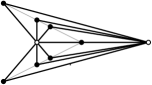
(a) $\rho^{1}_{2}(K_{2,q})\leq\lceil(3n-7)/2\rceil$.

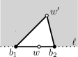
(b) $\rho^{1}_{2}(K_{2,q})\geq\lceil(3n-7)/2\rceil$.

Figure 9: Establishing lower and upper bounds for $\rho^{1}_{2}(K_{2,q})$.

Example 12

$\rho^{1}_{2}(K_{1,q})=\lceil m/2\rceil$ and $\rho^{1}_{2}(K_{2,q})=\lceil(3n-7)/2\rceil=\lceil(3m-2)/4\rceil$.

Proof

The former equality is obvious. We have to prove for $G=K_{2,q}$ that $\rho^{1}_{2}(G)=\lceil(3n-7)/2\rceil$. Fig. 9(a) shows that $\rho^{1}_{2}(G)\leq\lceil(n-3)/2\rceil+n-2=\lceil(3n-7)/2\rceil$. It remains to show the lower bound $\rho^{1}_{2}(G)\geq\lceil(3n-7)/2\rceil$. Suppose that our bipartition is defined by $2$ white vertices and $q$ black vertices. Associate the graph $G$ with its plane drawing. If there exist no line containing one white vertex and two black vertices of the graph $G$ then we need $m=2n-4\geq\lceil(3n-7)/2\rceil$ lines to cover all edges of the graph $G$. Assume from now that there exists a line $\ell$ containing a white vertex $w$ and two black vertices $b_{1}$ and $b_{2}$ of the graph $G$. Then the vertex $w$ lies on the line $\ell$ between the vertices $b_{1}$ and $b_{2}$. Let $w^{\prime}$ be the other white vertex. Since the point $w$ sees all black points, no one of them can be placed inside the shaded area, see Fig. 9(b). Then the point $w^{\prime}$ cannot be an interior point of a segment between two black points.

Thus all lines which cover at least two edges of the graph $G$ go through the point $w$, at most one of these lines go through the point $w^{\prime}$ and the remaining lines can cover only the edges incident to the vertex $w$. Now let $\mathcal{L}$ be a family of lines such that $|\mathcal{L}|=\rho^{1}_{2}(G)$ and each edge of the graph $G$ belongs to some line $\ell\in\mathcal{L}$. Let $\mathcal{L}_{w}=\{\ell\in\mathcal{L}:w\in\ell\}$, $\mathcal{L}_{w^{\prime}}=\{\ell\in\mathcal{L}:w^{\prime}\in\ell\}$, and $\mathcal{L}_{w,w^{\prime}}=\mathcal{L}_{w}\cap\mathcal{L}_{w^{\prime}}$. Clearly, $|\mathcal{L}_{w}|\geq\rho^{1}_{2}(K_{1,n-2})=\lceil(n-2)/2\rceil$. By the above, $|\mathcal{L}_{w^{\prime}}|=n-2$ and $|\mathcal{L}_{w,w^{\prime}}|\leq 1$. If the set $\mathcal{L}_{w,w^{\prime}}$ is empty, then $|\mathcal{L}|=|\mathcal{L}_{w}|+|\mathcal{L}_{w^{\prime}}|\geq\lceil(n-2)/2\rceil+n-2=\lceil(3n-6)/2\rceil$. If $\mathcal{L}_{w,w^{\prime}}=\{\ell_{0}\}$ then since the line $\ell_{0}$ covers exactly edges $(w,b)$ and $(w^{\prime},b)$ for some black vertex $b$, $|\mathcal{L}_{w}\setminus\{\ell_{0}\}|\geq\rho^{1}_{2}(K_{1,n-3})=\lceil(n-3)/2\rceil$, and $|\mathcal{L}|=|\mathcal{L}_{w}\setminus\{\ell_{0}\}|+|\mathcal{L}_{w^{\prime}}|\geq\lceil(n-3)/2\rceil+n-2=\lceil(3n-7)/2\rceil$. In both cases. $\rho^{1}_{2}(G)\geq\lceil(3n-7)/2\rceil$.

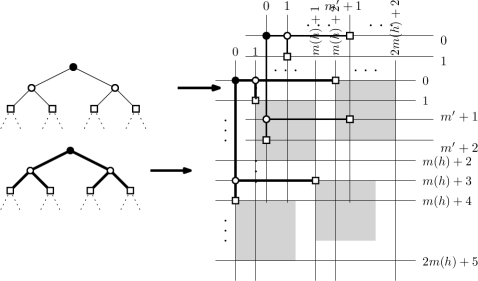
Figure 10: Drawing of a complete binary tree of height $h+2$ on a grid of size $(2m(h)+2)\times(2m(h)+5)$.

Example 13

If $G$ is the complete binary tree of height $h\geq 1$ consisting of $n$ nodes, then $\rho^{1}_{2}(G)>\sqrt{n-3}$. On the other hand, $\rho^{1}_{2}(G)\leq(6/{\sqrt{2}})\sqrt{n+1}-5$ if $h$ is even and $\rho^{1}_{2}(G)\leq 4\sqrt{n+1}-5$ otherwise.

Proof

Indeed, since $G$ has $(n-3)/2$ vertices with degree $3$, $\rho^{1}_{2}(G)>\sqrt{n-3}$ by Lemma 1(a).

To obtain an upper bound, let $m(2)=2$, $m(3)=4$, and $m(h+2)=2m(h)+4$ for $h\geq 2$. We prove by induction that we can draw the tree of height $h\geq 2$ on an $m(h)\times(m(h)+1)$-grid with the root placed at the top left corner (see also [23, Fig. 3(a)]). For the induction basis note that this is true for $h=2$ and $h=3$. We can also draw the tree of height $0$ on a $0\times 0$-grid and the tree of height $1$ on a $1\times 1$-grid, respectively, with the root placed at the top left corner. As the induction step, we use a $m(h+2)\times(m(h+2)+1)$ grid and place the root of the tree of height $h+2$ on the top left grid point $(0,0)$, place its child nodes on points $(1,0)$ and $(0,m(h)+3)$, and place its grandchild nodes on points $(m(h)+2,0)$, $(1,1)$, $(m(h)+1,m(h)+3)$ and $(0,m(h)+4)$ (see Fig. 10). For each grandchild $v$, consider the intersection of $m(h)$ gridlines to the right and the $m(h)+1$ gridlines to the bottom of $v$ (including the grid lines containing $v$). We reserve this part of the grid to the subtree of $v$. Note that every grid point is reserved to at most one grandchild due to the placement of the grandchild nodes. Since the subtree of a grandchild is a complete binary tree of height $h$, by induction, we can draw each of them in the reserved part of size $m(h)\times(m(h)+1)$ with the roots placed at the top left corners. Thus all edges of the tree of height $h$ belong to $2m(h)+1$ grid lines. We can easily show that $m(h)=6\cdot 2^{(h-2)/2}-4$ if $h\geq 2$ is even and $m(h)=8\cdot 2^{(h-3)/2}-4$ if $h\geq 3$ is odd. Since $n=2^{h+1}-1$, we get the claimed upper bounds.

Appendix 0.E Conclusion and Open Problems

Apart from the many open problems that we have mentioned throughout the paper, we suggest to study a topological version of $\rho^{l}_{d}$, say $\tau^{l}_{d}$, where there are $\tau^{l}_{d}(G)$ $l$-dimensional planes such that each edge of $G$ is contained in one such plane. It seems that $\tau^{1}_{d}(G)=\rho^{1}_{d}(G)$, and for $d\geq 3$, $\tau^{3}_{d}(G)=1$. So, the only interesting such parameter is $\tau^{2}_{3}(G)$. This would relate more closely to book embeddings.

Can we bound $\rho^{2}_{3}$ (and $\pi^{2}_{3}$) for 1-planar graphs or RAC graphs? Is $\rho^{2}_{3}$ bounded by a constant or linear function for bounded-degree graphs? Are there tighter bounds for $\rho^{2}_{3}(K_{n})$ than those in Theorem 2.4? Find $\lim_{n\to\infty}\rho^{2}_{3}(K_{n})/n^{2}$ if it exists.

Given that it is NP-complete to decide whether the vertex arboricity of a maximal planar graph is at most $2$ [27], how hard it is to test whether $\pi^{1}_{3}(G)=2$ for a planar graph $G$?

References

- [1] Akiyama, J., Era, H., Gervacio, S.V., Watanabe, M.: Path chromatic numbers of graphs. J. Graph Theory 13(5), 571–573 (1989)
- [2] Akiyama, J., Exoo, G., Harary, F.: Covering and packing ingraphs III: Cyclic and acyclic invariants. Math. Slovaca 30, 405–417 (1980)
- [3] Bannister, M.J., Devanny, W.E., Dujmović, V., Eppstein, D., Wood, D.R.: Track layouts, layered path decompositions, and leveled planarity (2015), http://arxiv.org/abs/1506.09145
- [4] Battista, G.D., Frati, F., Pach, J.: On the queue number of planar graphs. SIAM J. Comput. 42(6), 2243–2285 (2013)
- [5] Bollobás, B.: Combinatorics: Set Systems, Hypergraphs, Families of Vectors and Combinatorial Probability. Cambridge University Press, 1st edn. (1986)
- [6] Broere, I., Mynhardt, C.M.: Generalized colorings of outerplanar and planar graphs. In: Proc. 5th Int. Conf. Graph Theory Appl. Algorithms Comput. Sci., Kalamazoo, MI, 1984. pp. 151–161 (1985)
- [7] Brooks, R.L.: On colouring the nodes of a network. Mathematical Proceedings of the Cambridge Philosophical Society 37, 194–197 (4 1941)
- [8] Chan, T.M., Goodrich, M.T., Kosaraju, S.R., Tamassia, R.: Optimizing area and aspect ratio in straight-line orthogonal tree drawings. Comput. Geom. Theory Appl. 23, 153–162 (2002)
- [9] Chaplick, S., Fleszar, K., Lipp, F., Ravsky, A., Verbitsky, O., Wolff, A.: The complexity of drawing graphs on few lines and few planes (2016), http://arxiv.org/abs/1607.06444
- [10] Chartrand, G., Kronk, H.V.: The point-arboricity of planar graphs. J. Lond. Math. Soc. 44, 612–616 (1969)
- [11] Chen, Z., He, X.: Parallel complexity of partitioning a planar graph into vertex-induced forests. Discrete Appl. Math. 69(1-2), 183–198 (1996)
- [12] Di Battista, G., Frati, F.: Small area drawings of outerplanar graphs. Algorithmica 54(1), 25–53 (2007)
- [13] Dujmović, V.: Graph layouts via layered separators. J. Comb. Theory, Ser. B 110, 79–89 (2015)
- [14] Dujmović, V., Eppstein, D., Suderman, M., Wood, D.R.: Drawings of planar graphs with few slopes and segments. Comput. Geom. Theory Appl. 38(3), 194–212 (2007)
- [15] Dujmović, V., Morin, P., Wood, D.R.: Layout of graphs with bounded tree-width. SIAM J. Comput. 34(3), 553–579 (2005)
- [16] Dujmović, V., Pór, A., Wood, D.R.: Track layouts of graphs. Discrete Math. & Theor. Comput. Sci. 6(2), 497–522 (2004), http://www.dmtcs.org/volumes/abstracts/dm060221.abs.html
- [17] Dujmović, V., Whitesides, S.: Three-dimensional drawings. In: Tamassia, R. (ed.) Handbook of Graph Drawing and Visualization, chap. 14, pp. 455–488. CRC Press (2013)
- [18] Dujmović, V., Wood, D.R.: Three-dimensional grid drawings with sub-quadratic volume. In: Towards a theory of geometric graphs, pp. 55–66. AMS, Providence, RI (2004)
- [19] Durocher, S., Mondal, D.: Drawing plane triangulations with few segments. In: Proc. Canad. Conf. Comput. Geom. (CCCG’14). pp. 40–45 (2014), http://cccg.ca/proceedings/2014/papers/paper06.pdf
- [20] Felsner, S., Liotta, G., Wismath, S.: Straight-line drawings on restricted integer grids in two and three dimensions. J. Graph Algorithms Appl. 7(4), 363–398 (2003)
- [21] Flum, J., Grohe, M.: Parametrized Complexity Theory. Springer-Verlag, Berlin (2006)
- [22] de Fraysseix, H., Pach, J., Pollack, R.: How to draw a planar graph on a grid. Combinatorica 10(1), 41–51 (1990)
- [23] Garg, A., Rusu, A.: Straight-line drawings of binary trees with linear area and arbitrary aspect ratio. J. Graph Algorithms Appl. 8(2), 135–160 (2004)
- [24] Goddard, W.: Acyclic colorings of planar graphs. Discrete Math. 91(1), 91–94 (1991)
- [25] Graham, R.L., Knuth, D.E., Patashnik, O.: Concrete Mathematics: A Foundation for Computer Science. Addison-Wesley Publishing Group, Amsterdam, 2nd edn. (1994)
- [26] Grünbaum, B., Walther, H.: Shortness exponents of families of graphs. J. Comb. Theory, Ser. A 14(3), 364–385 (1973)
- [27] Hakimi, S., Schmeichel, E.: A note on the vertex arboricity of a graph. SIAM J. Discrete Math. 2, 64–67 (1989)
- [28] Hanani, H.: The existence and construction of balanced incomplete block designs. Ann. Math. Stat. 32, 361–386 (1961), http://www.jstor.org/stable/2237750
- [29] Harary, F.: Covering and packing in graphs I. Ann. N.Y. Acad. Sci. 175, 198–205 (1970)
- [30] Kostochka, A., Melnikov, L.: On a lower bound for the isoperimetric number of cubic graphs. In: Proc. 3rd. Int. Petrozavodsk. Conf. Probabilistic Methods in Discrete Mathematics, pp. 251–265. Moskva: TVP; Utrecht: VSP (1993)
- [31] Krein, M., Milman, D.: On extreme points of regular convex sets. Studia Math. 9, 133–138 (1940)
- [32] Matsumoto, M.: Bounds for the vertex linear arboricity. J. Graph Theory 14(1), 117–126 (1990)
- [33] Mohar, B., Thomassen, C.: Graphs on surfaces. John Hopkins University Press, Baltimore, MD (2001)
- [34] Pach, J., Thiele, T., Tóth, G.: Three-dimensional grid drawings of graphs. In: Di Battista, G. (ed.) Proc. 5th Int. Symp. Graph Drawing (GD’97). vol. 1353, pp. 47–51. Springer-Verlag (1997)
- [35] Poh, K.S.: On the linear vertex-arboricity of a planar graph. J. Graph Theory 14(1), 73–75 (1990)
- [36] Raspaud, A., Wang, W.: On the vertex-arboricity of planar graphs. Eur. J. Comb. 29(4), 1064–1075 (2008)
- [37] Ravsky, A., Verbitsky, O.: On collinear sets in straight-line drawings. In: Kolman, P., Kratochvíl, J. (eds.) Proc. 37th Int. Workshop Graph-Theoretic Concepts Comput. Sci. (WG’11). Lect. Notes Comput. Sci., vol. 6986, pp. 295–306. Springer-Verlag (2011), a preprint is available at http://arxiv.org/abs/0806.0253
- [38] Schaefer, M., Štefankovič, D.: Fixed points, Nash equilibria, and the existential theory of the reals. Theory Comput. Syst. pp. 1–22 (2015), has appeared online.
- [39] Schnyder, W.: Embedding planar graphs on the grid. In: Proc. 1st ACM-SIAM Symp. Discrete Algorithms (SODA’90). pp. 138–148 (1990)
- [40] Schulz, A.: Drawing graphs with few arcs. J. Graph Algorithms Appl. 19(1), 393–412 (2015)
- [41] Wang, J.: On point-linear arboricity of planar graphs. Discrete Math. 72(1-3), 381–384 (1988)
- [42] Wikipedia: Krein–Milman theorem, https://en.wikipedia.org/wiki/Krein-Milman_theorem, accessed April 21, 2016.
- [43] Wood, D.R.: Bounded-degree graphs have arbitrarily large queue-number. Discrete Math. & Theor. Comput. Sci. 10(1), 27–34 (2008), http://dmtcs.episciences.org/434
- [44] Wood, D.R.: Three-dimensional graph drawing. In: Kao, M.Y. (ed.) Encyclopedia of Algorithms, pp. 1–7. Springer-Verlag, Boston, MA (2008)