Minimalist Regression Network with Reinforced Gradients and Weighted Estimates: a Case Study on Parameters Estimation in Automated Welding

Abstract

This paper presents a minimalist neural regression network as an aggregate of independent identical regression blocks that are trained simultaneously. Moreover, it introduces a new multiplicative parameter, shared by all the neural units of a given layer, to maintain the quality of its gradients. Furthermore, it increases its estimation accuracy via learning a weight factor whose quantity captures the redundancy between the estimated and actual values at each training iteration. We choose the estimation of the direct weld parameters of different welding techniques to show a significant improvement in calculation of these parameters by our model in contrast to state-of-the-arts techniques in the literature. Furthermore, we demonstrate the ability of our model to retain its performance when presented with combined data of different welding techniques. This is a nontrivial result in attaining an scalable model whose quality of estimation is independent of adopted welding techniques.

I Introduction

I-A Overview

Automation of the welding processes witness a significant advancement in recent decades. This, in turn, introduces a dramatic improvement on the manufacturing productivity and its efficiency. As the interest in automation of this field of industry continues to grow, the needs for quality research on reducing the manual modification of its parameters by human operator becomes indispensable. For instance, most welding tasks involve fabrication of a large number of joints over an extended period of time where many of these joints require multiple welding passes. Furthermore, these tasks are mostly manual processes where the completion of a multi-pass welding for a single joint takes approximately a work shift, on average, by highly skilled welders. This limits the productivity of companies since there exists a limited number of welders with such a skill. Moreover, many of such welding tasks take place in outdoor environment whose conditions are hostile to human health. Therefore, the automation of this fabrication process is highly desirable.

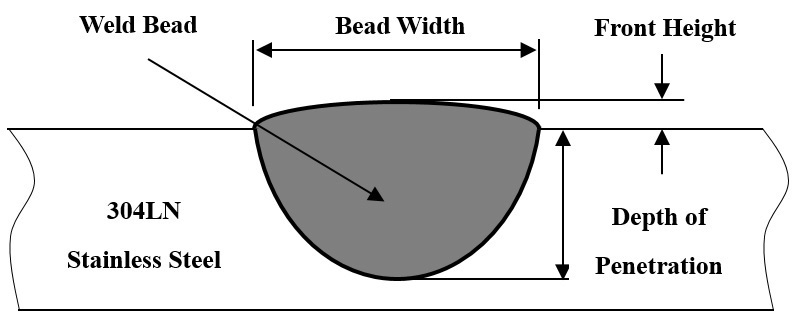
Figure 1: Bead width and depth of penetration as examples of Direct Weld Parameters (DWP). The weld bead along with its front height on 304LN stainless steel is shown in the figure.

The intelligent monitoring of the welding process helps increase the precision and accuracy of the various aspects of its final outcome (e.g., the geometry of the weld beads). Furthermore, it helps determine if the driving parameters of the welding system requires readjustment. As a result, the overall performance of the system and consequently its welding quality improves significantly.
Welding is an integral part of virtually every industrial process, from construction of buildings and complex structures to automotive and shipyard production lines. This explains the existence of a wide range of welding techniques from Gas Metal Arc Welding (GMAW) [1] and Sub-merged Arc Welding (SAW) [2] to shielded metal-arc welding (SMAW) [3], Tungsten Insert Gas Welding (TIG) [4], and Gas Tungsten Arc Welding (GTAW) [5].
A welding task, in its common form, comprises of a number of input control signals. Some examples include the voltage, the current, the torch traveling speed, the wire feed rate, and the arc gap. Cook [6] uses the term Indirect Weld Parameters (IWP) to refer to these input control signals. Furthermore, Nunes [7] shows that IWP directly influence the geometrical description of the welding pool i.e., its Direct Weld Parameters (DWP) [6]. The depth of penetration, the width of weld beads, and the transverse cross-sectional areas are some of the examples of these parameters. Firgure 1 illustrates these parameters for a weld bead on a 304LN stainless steel. A thorough investigation of the relationship between DWP and IWP is presented by Chandel and Bala [8].
Research pertaining to welding processes is broadly categorized into two domain of studies, namely the estimation of the weld parameters and their sensitivity analysis. The latter refers to the study of the effect of the changes of IWP on the final weld quality. Whereas, the estimation problem attempts to predict the weld parameters, given the IWP. In this article, we focus on the estimation problem.
Rosenthal [9] presents an early static model based on heat flow where the welding contour is expressed as a function of electrode velocity, heat input, and the material properties. In addition, many researchers apply sophisticated mathematical models to capture this relationship. Some examples include factorial design [10, 11, 12], linear regression [13, 1], multiple regression analysis [14], response surface methodology [15], and Taguchi method [16, 17].

I-B Artificial Neural Networks and Automated Welding

Research on Artificial Neural Network (ANN) has witnessed a tremendous success in the past two decades. These computational models have been deployed in a wide range of applications from natural language processing [18] to object tracking [19]. In their industrial applications, automated welding is where these models have specially proven successful. In particular, the ability of these models to generalize on a broad range of inputs makes them an attractive choice, given the existence of a wide range of welding techniques . In addition, ANN provides a powerful and accurate alternative to highly sophisticated yet domain-specific approaches such as heat flow [9], factorial design [1], response surface methodology [20], and support vector regression [21, 22].
Application of ANN in estimation of the weld bead parameters bring a remarkable progress in recent years. These models are successfully deployed in investigation of the modeling, the process control, and the estimation of the quality of the weld beads [23]. Anderson et al. [5] investigate the application of multi-layer neural networks in modeling of the arc welding process. They achieve satisfactory results in their prediction accuracy as compared to the conventional control systems. Tang et al. [24] apply back-propagation and counter-propagation to analyze the relationship between IWP and the geometry of the weld bead in TIG welding. Polte et al. [25] consider the application of the self-organizing maps (SOM) in monitoring and quality evaluation of the GMAW welding. Nagesh and Datta [3] apply back-propagation on modeling and estimation of the weld bead parameters in SMAW. Chandrasekhar and Vasudevan [26] combine their neural network with genetic algorithm for post-optimization of the estimated parameters of their network. Their model achieves a considerable improvement in optimization of these parameters in A-TIG welding. Benyounisa and Olabi [27] present a comprehensive survey on optimization techniques for estimation of the direct weld parameters.

I-C Challenges and Limitations

One challenging aspect of this estimation problem is the dependency of DWP on the same input control signals or IWP. For instance, the same set of values of voltage, current, and torch traveling speed (i.e., IWP) produces the different values that pertain to the depth of penetration and the width of weld beads (i.e., DWP). Therefore, it is of no value to combine these parameters in a single output vector to estimate their values. This is mainly due to the pseudo-redundancy caused by the overlapping values of input feature vectors for different output data. This is particularly problematic when applying backpropagation [28] due to the saturation behavior of the common activation functions in neural networks [29]. Utilization of the rare features to craft domain-specific feature weightings, such as TF-IDF [30] is a solution to tame this limitation. However, the inherent low-dimensionality of IWP feature vectors (with voltage, current, and torch traveling speed among the most common values) does not guarantee the applicability of this solution in the domain of welding. This limits the ability of estimation models to establish a well-generalized mapping of different DWP onto the same set of IWP values. Although some models attempt to compensate for such shortcomings through introduction of polynomial features, such polynomial degrees do not necessarily guarantee a better estimation of DWP values [12, 20].
On the other hand, adaptive gradient or adagrad dynamically incorporates knowledge of the geometry of data that is observed in earlier iterations in order to achieve more informative gradient-based learning [31]. However, the weak correlation among DWP (please refer to Figure 4) does not allow the inference of the value of one (e.g., depth of penetration) from the other (e.g., width). Furthermore, some approaches apply noise to the activation function [32, 33] for feed-forward networks and Boltzmann machines [34] to encourage deeper exploration by neural units, thereby easing the optimization of their corresponding outcomes. However, these approaches face vanishing gradient information due to the saturation of these units [29]. Although rmsprop [35] shows impressive results and improvements [36], there is not much understanding for its success in practice [37]. Momentum is another approach to increase speed of convergence. It damps the size of gradient steps along the directions of high curvature while yielding a larger effective learning rate along the directions of low curvature [38]. As a result, it ensures faster convergence [39, 40] compared to stochastic gradient descent in convex optimization problems [29]. Thorough investigation of adopted techniques for backpropagation and gradient based training are found in [28, 41].

I-D Contributions

Our contributions to address these challenging issues are:

1. We resolve the vanishing gradient of our model through introduction of a new meta-parameter, referred to as reinforced learning coefficient, to enable this model to maintain the quality of its computed gradients. Our approach is comparable to Gulcehre et. al [29]. Whereas, they apply an additive noise to the input or output layers, the multiplicative nature of our parameter that is directly applied to the calculated gradients magnifies the exponent of the activation function in next iteration, thereby sharpening its transition. In addition, we model a minimalist single-layer neural regression model as opposed to a deep neural network for classification in their study.

2. We further reduce the estimation error of our model using a weighted regression estimator at its output layer and learning the state of this weight.

3. we show the scalability of our model on combination of datasets of different welding techniques. In particular, we show that the change in estimation error exhibited by our model due to combination of data of these welding techniques is statistically insignificant. This is a non-trivial result that challenges the general belief in this field of research. However, we acknowledge that our result is, by no means, a definitive solution but an early attempt to formulation of one such scalable model.

It is worth noting that we tame the effect of low-dimensionality of IWP by readjusting the number of neurons of the hidden layer of the respective blocks of our model at runtime and in consecutive training epochs. This enables our model to better capture the interrelation between individual elements of the input feature vectors (i.e., IWP), thereby eliminating the needs for further polynomial features [12, 20]. Additionally, we present a comprehensive comparative study of our model in contrast to state-of-the-art techniques in the literature to show a significant improvement in estimation of direct weld parameters.
The remainder of this article is organized as follows. Section II explains the overall architecture and the formulation of our neural regression network. We present the results of performance of our model in Section III. In section IV, we study the effect of increase in hidden layers on estimation quality of our model. Section V elaborates on scalability of our model on combined data of different welding techniques. Conclusion and some insights on future direction of this research are presented in Section VI.

II Neural Architecture

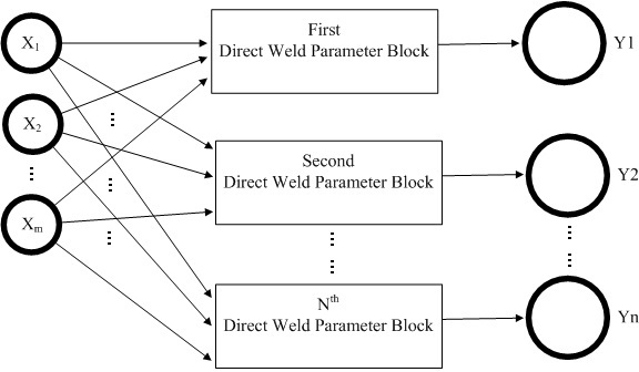
Figure 2: Overall Architecture. Each block is a one-layer neural regression network whose set of meta-parameters and direct weld parameter are independent of other blocks. IWP form the input features to the entire model.

We model our minimalist neural architecture as an aggregate of independent one-hidden-layer regression blocks as depicted in Figure 2. Number of these blocks is proportional to cardinality of DWP. For instance, it is a two-block regression model if DWP are depth of penetration and width of weld beads. These blocks are trained simultaneously and share an identical structure as shown in Figure 3. In particular, they apply Sigmoid activation function on IWP feature vectors and generate their corresponding outputs through application of linear transformation function on calculated values of their respective hidden layer. This enables each block to act as an independent non-linear regression network. Initially, the hidden layer of a given block is assigned with two neural computation units. During the training, our model modifies the size of this hidden layer if such an update results in further improvement of their respective estimated values.

Figure 3: Block-level neural architecture. n is the total number of blocks (i.e., cardinality of DWP) and k indicates the number of neurons on a hidden layer. The weight matrices $\Theta^{(i,n)},~{}i=1,2$ are unique to their blocks.

Let $X$ denote the set of feature vectors (i.e., IWP) to our model. Furthermore, let $Y^{(k)}$ and $H^{(k)}$ represent the set of direct weld parameter and the hidden layer of the $k^{th}$ block of this architecture, with $k=1,\dots,N$, where N is the cardinality of DWP. Moreover, let $\Theta^{(r,k)},~{}r=1,2$, be the weight matrices that are associated with the $k^{th}$ block. Values that are generated at the hidden layer of the $k^{th}$ block are:

$$\begin{split}z^{(1,k)}=X^{T}\times\Theta^{(1,k)}\end{split}$$ (1)

$$\begin{split}H^{(k)}=\frac{1}{1+e^{-z^{(1,k)}}},~{}k=1,\dots,N\end{split}$$ (2)

where N is the cardinality of DWP. The final weighted estimates of these blocks at $t^{th}$ iteration of the training are:

$$Y^{\prime(k,t)}=[(H^{(k)})^{T}\times\Theta^{(2,k)}]+\tau^{(k,t)}$$ (3)

$\Theta^{(2,k)}$ is the weight matrix between the hidden layer of the $k^{th}$ block and its output layer. $\tau^{(k,t)}$ in equation (3) is the weight associated with the regression estimator at the output layer of the $k^{th}$ block whose value is learned during the training phase:

$$\tau^{(k,t)}=\{-\nu,0,\nu\}$$ (4)

$$\nu=\frac{1}{m}(Y^{\prime(k,t-1)}-Y^{(k)})$$ (5)

subject to:

$$\min[\frac{1}{2m}[(Y^{(k)}-Y^{\prime(k,t)})^{2}+\lambda^{(k)}\sum_{r=1}^{2}\sum_{i=1}^{p^{(r,k)}}\sum_{j=1}^{q^{(r,k)}}(\Theta^{(r,k)}_{ji})^{2}]]$$ (6)

In other words, the value of this weight varies between zero and $\pm$ mean of actual estimation errors at $t-1$ iteration of the training, given its positive impact on minimization of the regularized cost function of its respective regression block as formulated in equation (6). The entries of $Y^{\prime(k,t-1)}$ in equation (5) are initialized to zero at $t=1$ and m is the total number of training data. The second term in equation (6) is the regularization term that incorporates the sum of the squared of the weight matrices in the $k^{th}$ block to prevent overfitting on its corresponding direct weld parameter. $\lambda^{(k)}$ is its regularization factor. $p^{(r,k)}$ and $q^{(r,k)},~{}r=1,2$ refer to the row and the column dimensions of the weight matrices of the $k^{th}$ block, respectively. It is worth noting that we add an extra column with all whose entries equals to 1 to X and $H^{(k)}$ to count for the bias term. This is why we do not explicitly include this term in equation (1). This also explains the starting indices of the last two summation operations from 1 in equation (6).
The discrepancies between these weighted estimates in equation (3) and the actual DWP at $t^{th}$ training iteration are:

$$\delta^{(Y^{(k)})}=Y^{(k)}-Y^{\prime(k,t)},~{}k=1,\dots,N$$ (7)

We use these values to update $\Theta^{(2,k)}$:

$$\begin{split}\Delta^{(2,k)}=((\delta^{(Y^{(k)})})^{T}\times H^{(k)})\times\gamma^{(k)}\end{split}$$ (8)

$$\begin{split}\Theta^{(2,k)}=\Theta^{(2,k)}+\frac{1}{m}(\alpha^{(k)}\times\Delta^{(2,k)}+\lambda^{(k)}\sum_{i=1}^{p^{(2,k)}}\sum_{j=1}^{q^{(2,k)}}\Theta^{(2,k)}_{ji})\end{split}$$ (9)

where m is the total number of training data and $k=1,\dots,N$ reflects the total number of blocks (i.e., cardinality of DWP) in our model. $p^{(2,k)}$ and $q^{(2,k)}$ refer to the dimensions of the weight matrix of the linear transformation layer of $k^{th}$ block. Equation (8) is the gradient of this output layer and $\gamma^{(k)}$ is the reinforced learning coefficient of the $k^{th}$ block. In essence, $\gamma^{(k)}$ is a standard normal multiplicative factor (i.e., $((\sigma^{2}\times\gamma^{(k)})+\mu)\sim\mathcal{N}(\mu=0,\sigma^{2}=1)$) that is learned during the training and is shared by all the layers of a given block. It magnifies the exponent of the Sigmoid function in each consecutive iteration via perturbing the gradients of the previous step during the training, thereby maintaining stronger gradients.This allows our model to further reduce its deviation from the expected DWP to significantly minimize its estimation error. Furthermore, $\alpha^{(k)}$ and $\lambda^{(k)}$ are the learning rate and the regularization factor of the corresponding independent set of meta-parameters of $k^{th}$ block, respectively. Similarly, the update of the weight matrix $\Theta^{(1,k)}$ is:

$$\begin{split}\delta^{(2,k)}=((\Theta^{(2,k)})^{T}\times\delta^{(Y^{(k)})})\times(H^{(k)}\times(1-H^{(k)}))\\ ,~{}k=1,\dots,N\end{split}$$ (10)

$$\begin{split}\Delta^{(1,k)}=((\delta^{(2,k)})^{T}\times X)\times\gamma^{(k)}\end{split}$$ (11)

$$\begin{split}\Theta^{(1,k)}=\Theta^{(1,k)}+\frac{1}{m}(\alpha^{(k)}\times\Delta^{(1,k)}+\lambda^{(k)}\sum_{i=1}^{p^{(1,k)}}\sum_{j=1}^{q^{(1,k)}}\Theta^{(1,k)}_{ji})\end{split}$$ (12)

where $(H^{(k)}\times(1-H^{(k)}))$ in equation (10) is the gradient of the Sigmoid activation function of the $k^{th}$ block.

III Case Study

We compare the performance of our minimalist neural regression network in contrast to a number of selected studies in the literature. In particular, we choose Anderson et al. [5], Chandrasekhar and Vasudevan [26], Karaoglu and Secgin [2], Chotěborský et.al [43], and Dhas and Satheesh [42]. These articles form a reliable representatives of the trends of research in this field over the past two and a half decades. More specifically, [5] is the seminal paper that introduces the application of multi-layer neural networks in estimation of the direct weld parameters. Furthermore, Karaoglu and Secgin [2] adopt a curvilinear approach to estimation of DWP. Moreover, Chandrasekhar and Vasudevan [26] propose a combination of single hidden layer neural network and genetic algorithm for post-optimization of the estimated DWP. In addition, Chotěborský et.al [43] and Dhas and Satheesh [42] present (to the best of our knowledge) the highest estimation accuracy in application of the classical models, Taguchi method and factorial design respectively, in the literature. Furthermore, their welding data that are publicly available, pertain to four main welding techniques, namely:

1. $D_{1}$: Anderson et al. [5] on arc welding process.

2. $D_{2}$: Karaoglu and Secgin [2] on submerge arc welding (SAW).

3. $D_{31}$ and $D_{32}$: Chandrasekhar and Vasudevan [26] datasets on Tungsten insert gas welding (A-TIG) welding on 304LN and 316LN stainless steel, respectively.

4. $D_{4}$: Dhas and Satheesh [42] dataset on Taguchi method on SAW.

5. $D_{5}$: Chotěborský et.al [43] dataset on factorial design technique on gas metal arc welding (GMAW).

Figure 4 shows the regression fit to the depth of penetration and width of weld beads in $D_{1}$. Their Pearson correlation ratio along with its p-value are $\{0.12,-0.24\}$. Furthermore, those of Spearman and Kendall for these DWP are $\{0.05,-0.31\}$ and $\{0.09,-0.17\}$, respectively. These correlation ratios show a weak proportionality between the values of these DWP. Furthermore, their p-values reject the null hypothesis of correlation between these DWP at $0.05$ and $0.01$ significance levels. This is in accordance with our claim in section I-C of this article. Moreover, this trend of absence of correlation between DWP is exhibited in $D_{2}$ through $D_{5}$.
Tables I and II reveal the overall simplicity of our minimalist neural regression model. More specifically, the cumulative number of neurons of the two blocks of our model that are dynamically selected at runtime from range $\{2,\dots,100\}$, does not exceed

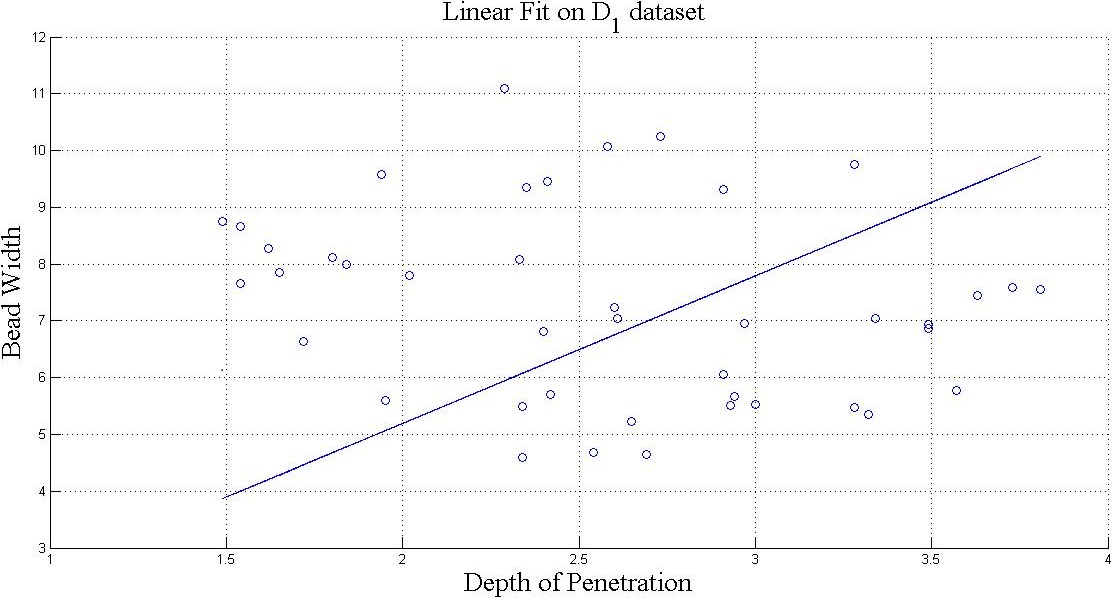
Figure 4: Regression fit on $D_{1}$ [5], demonstrating a weak correlation between depth of penetration and width of weld beads.

TABLE I: Best meta-parameters - depth of penetration block.

Datasets	Neurons $\in[2,\dots\\ ,100]$	Degree	$\alpha$	$\gamma$	$\lambda$	Iterations $\in[1000,\dots\\ ,12000]$
$D_{1}$	4	0	40.0	0.9	0.0	1000
$D_{2}$	8	0	100	0.1	0.001	1000
$D_{31}$	5	0	30	1.0	0.0	9000
$D_{32}$	9	0	0.009	2500	0.0	7000

TABLE II: Best meta-parameters - width of weld beads block.

Datasets	Neurons $\in[2,\dots\\ ,100]$	Degree	$\alpha$	$\gamma$	$\lambda$	Iterations $\in[1000,\dots\\ ,12000]$
$D_{1}$	2	0	0.01	2500	0.0	9000
$D_{2}$	3	0	0.009	2000	0.003	1000
$D_{31}$	4	0	0.3	1500	0.0	1000
$D_{32}$	3	0	50	0.5	0.001	1000

Figure 5: Effect of the Reinforced Learning Coefficient $\gamma$ on gradients of the weight matrix $\Theta^{(1,k)},~{}k=1$ i.e., depth of penetration block.

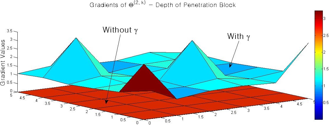
Figure 6: Effect of the Reinforced Learning Coefficient $\gamma$ on gradients of the weight matrix $\Theta^{(2,k)},~{}k=1$ i.e., depth of penetration block.

12 neurons in total (with mean and standard deviation of 9.50 and 2.65). It is interesting to note that the best results reported in [5] correspond to a $2\times 18$ networks (i.e., 36 neurons in total). Moreover, our model does not require any polynomial features (examined in the range $\{0,\dots,6\}$). This considerably reduces its training time. Additionally, it does not suffer from overfitting as indicated by significantly small entries of regularization parameter $\lambda$ in these tables, with most of whose entries equal zero.
Moreover, these tables reveal the inverse proportionality of the values of the learning rate $\alpha$ and the reinforced learning coefficient $\gamma$. This implies that the readjustment of the gradients of the weight matrices of our model results in better compensation for the variance that is exhibited by the input feature vectors (i.e., IWP). Figures 5 and 6 illustrate the effect of the reinforced learning coefficient $\gamma$ on gradients of the weight matrices $\Theta^{(i,k)},~{}i,=1,~{}2,~{}~{}k=1$ i.e., depth of penetration block of our model. Furthermore, the evolution of the learned weight values i.e., $\tau^{(k,t)}$ in equation (3) for depth of penetration and the width of weld beads blocks of our model are shown in figures 7 and 8, respectively.
However, variations in number of iterations during the training (with mean and standard deviation of (4500, 4123.1) and (3000, 4000.0) for depth of penetration and width of weld beads, respectively) do not exhibit any particular pattern or correspondence with the size of given datasets or the DWP. As a result, any conclusion on the effect of the size of the dataset or type of direct weld parameter on training process is not warranted. However, it takes longer, on average, for our model to converge on depth of penetration as compared to width of weld beads.

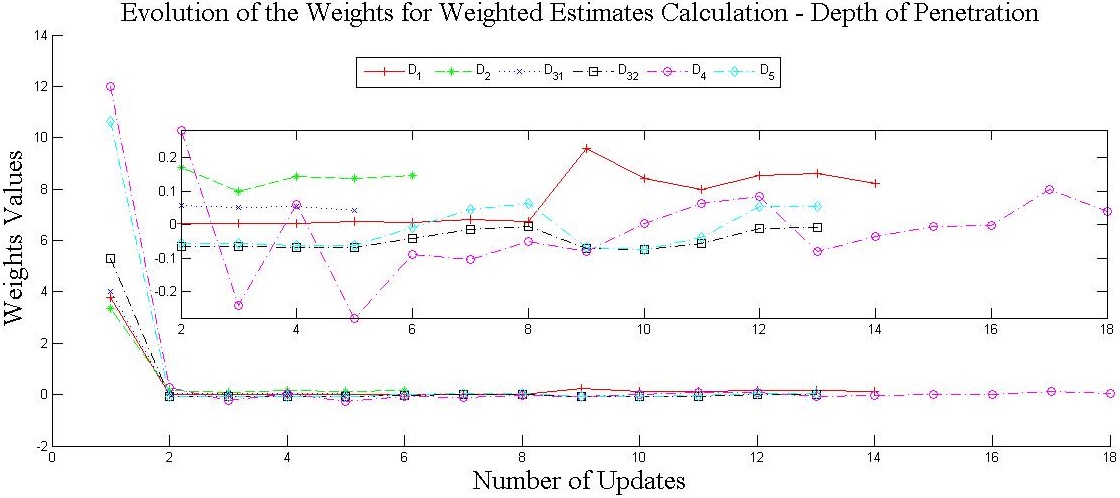
Figure 7: Evolution of weight values i.e., $\tau^{(k,t)}$ in equation (3) of weighted estimates for Depth of Penetration regression block on datasets $D_{1}$ through $D_{5}$.

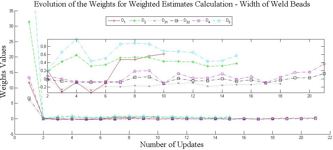
Figure 8: Evolution of weight values i.e., $\tau^{(k,t)}$ in equation (3) of weighted estimates for Width of Weld Beads regression block on datasets $D_{1}$ through $D_{5}$.

III-A Comparison with Selected Literature

Tables III through VIII show the results of the performance of our minimalist neural regression network (NRN in these tables) on test data in comparison with results reported in $D_{1}$, $D_{2}$, $D_{31}$, $D_{32}$, $D_{4}$, and $D_{5}$. In addition to these results, we also report the performance of our neural regression network in contrast with support vector regression (SVR) [21, 22], and neural network without application of our proposed reinforced learning coefficient with weighted estimates in equations (3), (8), and (11), (i.e., ANN entry of these tables). It is worth noting that we use the Python scikit-learn package [44] for modelling SVR. It achieves its best results using the polynomial degree activation function (i.e., poly) with four added polynomial features. Moreover, we choose Root Mean Squared Error (RMSE) and the percentage of Prediction Error (PE) to report our results. We calculate the PE of our model as:

$$\begin{split}PE=\frac{|Y^{(k)}-Y^{\prime(k,T)}|}{Y^{(k)}}\times 100\end{split}$$ (13)

where $Y^{(k)}$ and $Y^{\prime(k,T)}$ are the actual and estimated direct weld parameter of the $k^{th}$ block and $|.|$ gives the absolute value of its argument. T in $Y^{\prime(k,T)}$ indicates the final estimated value of the $k^{th}$ block at time T. We choose RMSE and PE to allow the comparative analysis of our results with respect to the selected literature. More specifically, Anderson et al. [5] and Dhas and Satheesh [42] report the PE of their models. Whereas, Karaoglu and Secgin [2] and Chandrasekhar and Vasudevan [26] provide RMSE as a measure of accuracy of their models. Furthermore, Chotěborský et.al [43] report Mean Squared Error (MSE) of their model. However, we include square root of these values i.e., RMSEs of their model.
A comparison between the PE values in Table III reveals that the differences between these values are above one

TABLE III: RMSEs and PEs - neural regression network (NRN) vs. $D_{1}$, support vector regression (SVR), and regular artificial neural network (ANN).

	Penetration (mm)	Width
	$RMSE$	$PE$	$RMSE$	$PE$
$D_{1}$	-	19.58%	-	5.68%
NRN	0.085	3.59%	0.073	2.91%
SVR	0.34	25.80%	0.26	23.13%
ANN	0.17	11.62%	0.28	24.61%

standard deviation (9.65 and 11.37, respectively). As a result, the reduction of the percentage of the prediction error by our model on this dataset is significant. Additionally, the RMSE values that are calculated by our model are considerably small (in the scale of millimeter). However, we are unable to confirm the significance of these values since the RMSEs of the multi-layer network in [5] are not reported.
We notice the same trend of improvement on the entries of Tables IV through VI. More specifically, Table IV shows that our model achieves more than 8 times improvements on RMSE values compared to $D_{2}$, with its corresponding z-score above one standard deviation (it is 1.382 and -1.457 for depth of penetration and width of weld beads, respectively). Moreover, the PE values reported in this table are significantly small with whose difference above one standard deviation from those of SVR and ANN (6.801 and 5.596 for depth of penetration and width of weld beads). However, we cannot draw any conclusion on its significance with respect to [2] since

TABLE IV: RMSEs and PEs - neural regression network (NRN) vs. $D_{2}$, support vector regression (SVR), and regular artificial neural network (ANN).

	Penetration (mm)	Width
	$RMSE$	$PE$	$RMSE$	$PE$
$D_{2}$	0.292	-	0.353	-
NRN	0.034	0.85%	0.041	0.94%
SVR	0.14	10.18%	0.11	9.13%
ANN	0.06	2.75%	0.16	7.43%

they do not provide PEs of their model. Similarly, Tables V and VI report the improvements of the RMSE values that range between 1.62 - 3.01 and 3.35 - 3.81 times, compared to results obtained in $D_{31}$ and $D_{32}$, respectively. Moreover, the PE values of these tables are above one standard deviation (i.e., (4.86, 4.24) and (5.81, 5.09) for entries of Tables V and VI, respectively). Additionally, these improvements are the direct results of our minimalist neural regression network using reinforced learning coefficient and weighted estimates, without application of any post-optimization of the estimated values using genetic algorithm, as reported by Chandrasekhar and Vasudevan [26]. Additionally, our model achieves 1.40 and 4.28 times improvements on depth of penetration and width of weld beads in $D_{4}$ , with their difference above one standard deviation (it is 2.340) on width of weld beads, as shown in Table VII. Furthermore, the z-score of its RMSEs are above one standard deviation from those calculated by SVR and ANN (they are -1.154 and -1.126, respectively). However, we are unable to report the significance of these RMSEs with respect to results in $D_{4}$ since Dhas and Satheesh [42] do not present these values on their model. Similarly our model outperforms results by Chotěborský et.al [43] in $D_{5}$ by a large margin i.e., 9.5 and 15 times improvements on DWP, as shown in Table VIII.
Moreover, the overlapping interval at $95\%$ confidence level in Table IX indicates that differences between the results obtained by our model on these datasets is insignificant. In other words, our minimalist model using reinforced learning coefficient with weighted estimates is capable of generalizing on features of different welding techniques. This observation is further supported by the minor differences in the meta parameters associated with these datasets on Tables I and II.

TABLE V: RMSEs and PEs - neural regression network (NRN) vs. $D_{31}$, support vector regression (SVR), and regular artificial neural network (ANN).

	Penetration (mm)	Width
	$RMSE$	$PE$	$RMSE$	$PE$
$D_{31}$	0.148	-	0.205	-
NRN	0.091	2.65%	0.068	1.94%
SVR	0.299	10.18%	0.159	9.13%
ANN	0.263	11.75%	0.165	9.43%

TABLE VI: RMSEs and PEs - neural regression network (NRN) vs. $D_{32}$, support vector regression (SVR), and regular artificial neural network (ANN).

	Penetration (mm)	Width
	$RMSE$	$PE$	$RMSE$	$PE$
$D_{32}$	0.124	-	0.156	-
NRN	0.037	0.93%	0.041	1.04%
SVR	0.246	13.48%	0.193	11.66%
ANN	0.226	11.75%	0.165	9.43%

TABLE VII: RMSEs and PEs - neural regression network (NRN) vs. $D_{4}$, support vector regression (SVR), and regular artificial neural network (ANN).

	Penetration (mm)	Width
	$RMSE$	$PE$	$RMSE$	$PE$
$D_{4}$	-	1.27%	-	4.32%
NRN	0.026	0.91%	0.037	1.01%
SVR	0.258	14.48%	0.212	12.66%
ANN	0.267	10.75%	0.172	8.94%

TABLE VIII: RMSEs and PEs - neural regression network (NRN) vs. $D_{5}$, support vector regression (SVR), and regular artificial neural network (ANN).

	Penetration (mm)	Width
	$RMSE$	$PE$	$RMSE$	$PE$
$D_{5}$	0.228	-	0.570	-
NRN	0.024	0.75%	0.038	0.84%
SVR	0.18	10.28%	0.15	9.64%
ANN	0.069	3.01%	0.172	8.12%

TABLE IX: RMSE Confidence Interval (95%) - minimalist neural regression network (NRN) on $D_{1}$, $D_{2}$, $D_{31}$, $D_{32}$, $D_{4}$, and $D_{5}$.

	$Penetration$	$Width$
$D_{1}$	(0.019, 0.143)	(0.031, 0.155)
$D_{2}$	(-0.031, 0.102)	(-0.040, 0.084)
$D_{31}$	(0.051, 0.175)	(-0.008, 0.120)
$D_{32}$	(-0.019, 0.110)	(-0.006, 0.118)
$D_{4}$	(-0.017, 0.108)	(-0.004, 0.113)
$D_{5}$	(-0.015, 0.098)	(-0.004, 0.114)

III-B Comparison with Adagrad, Rmsprop, and Nesterov Momentum

We compare the performance of our minimalist model using reinforced learning coefficient with weighted estimates in equations (3), (8), and (11) in contrast with neural network using adagrad [31], rmsprop [35], and Nesterov momentum [39] for backpropagation and weight updates. Increase in the average number of neural units is the first difference between our approach and these techniques. Whereas, number of neurons in our model does not exceed 12 units in total (with mean and standard deviation of 9.50 and 2.65) as shown in Tables I and II, the average number of neurons is more than 70 for a model using these alternative techniques. Furthermore, our approach achieves a considerable improvements on calculating RMSEs as compared to their results as shown in Tables X and XI. In particular, such an improvement is significant when we compare our approach with Nesterov momentum for both, depth of penetration and width of weld beads, with their difference above one standard deviation, on average (2.617 and 2.617, respectively). Moreover, performance of adagrad and rmsprop on these datasets are equivalent. The average z-score of the performance of our approach is above one standard deviation of RMSEs computed by adagrad and rmsprop (their z-score values are [-1.149 0.483 0.666] and [-1.130, 0.363, 0.767] for depth of penetration and width of weld beads for our model, adagrad and rmsprop, respectively). Additionally, our model achieves, on average, 2.817 and 2.871 times improvements on depth of penetration and 4.868 and 5.153 on width of weld beads. As a result, these improvements exhibited by our model are statistically significant.

TABLE X: RMSEs - neural regression network (NRN) vs. neural network using adagrad, rmsprop, and Nesterov Momentum.

	Depth of Penetration (mm)
	$NRN$	$adagrad$	$rmsprop$	$Nesterov$
$D_{1}$	0.085	0.173	0.186	3.435
$D_{2}$	0.034	0.091	0.091	3.261
$D_{31}$	0.091	0.267	0.186	4.139
$D_{32}$	0.037	0.125	0.224	3.593
$D_{4}$	0.026	0.165	0.218	3.942
$D_{5}$	0.024	0.138	0.233	3.867

TABLE XI: RMSEs - neural regression network (NRN) vs. neural network using adagrad, rmsprop, and Nesterov Momentum.

	Width of Weld Beads (mm)
	$NRN$	$adagrad$	$rmsprop$	$Nesterov$
$D_{1}$	0.073	0.362	0.368	3.630
$D_{2}$	0.041	0.291	0.332	3.856
$D_{31}$	0.068	0.352	0.341	4.026
$D_{32}$	0.041	0.123	0.085	3.215
$D_{4}$	0.037	0.146	0.223	4.108
$D_{5}$	0.038	0.152	0.203	3.675

TABLE XII: Neurons per hidden layer and the Iterations - Average performance of NRN with $1,\dots,~{}4$ hidden layers on $D_{1}$ through $D_{5}$.

	Penetration (mm)	Width
	$Nrns$	$Iters$	$Nrns$	$Iters$
$1H$	6.5	4500	3	3000
$2H$	7	7000	6	5000
$3H$	9	7000	7	1000
$4H$	9	6000	7	4000

IV Effect of Number of Hidden Layers on Quality of Estimation

Table XII presents average number of neural units (per hidden layer) as well as average iterations for training our model on $D_{1}$ through $D_{5}$, with its number of hidden layers varying in range $[1,\dots,4]$. It is worth noting that our experiment with increased number of hidden layers indicates that the estimated values rapidly degrade, trapping in a zero-gradient regime, once the number of hidden layers exceeds four. Therefore, we do not report on architecture with more than four hidden layers.
Table XII shows that the difference between the number of neurons of these architectures for depth of penetration and width of weld beads are above one standard deviation (1.315 and 1.893, respectively). Moreover, number of iterations to train these models proportionally increases with an increase in number of hidden layers, in case of depth of penetration. However, this observation does not hold in case of width of weld beads.
A comparison between the RMSE and PE values of these models in Table XIII for depth of penetration and width of weld beads reveals that their corresponding values are within one standard deviation from each other (they are (0.003, 0.436) and (0.0024, 0.642) for RMSE and PE values). In addition, Table XIV shows that the confidence interval of these models for $95\%$ level are all overlapping. As a result, an increase in the number of hidden layers of our minimalist neural regression network does not guarantee a significant improvement on its performance for estimation of DWP of the welding processes. Therefore, the minimalist design of our neural regression network does not jeopardize its quality of estimation.

TABLE XIII: RMSEs and PEs - Average performance of NRN with $1,\dots,~{}4$ hidden layers on $D_{1}$ through $D_{5}$.

	Penetration (mm)	Width
	$RMSE$	$PE$	$RMSE$	$PE$
$1H$	0.061	2.005%	0.055	1.707%
$2H$	0.069	2.98%	0.052	2.40%
$3H$	0.061	2.87%	0.052	3.19%
$4H$	0.063	2.58%	0.057	2.86%

TABLE XIV: Confidence Interval (95%)- Average performance of NRN with $1,\dots,~{}4$ hidden layers on $D_{1}$ through $D_{32}$.

	$Penetration$	$Width$
$1H$	(-0.001, 0.122)	(-0.0069, 0.116)
$2H$	(0.007, 0.131)	(-0.0099, 0.114)
$3H$	(-0.001, 0.122)	(-0.0099, 0.114)
$4H$	(0.001, 0.125)	(-0.0049, 0.119)

V Scalability on Combined Data

This section provides result of performance of our model on combination of $D_{1}$ through $D_{5}$ to show its scalability on different welding techniques. We refer to this combined dataset as $D_{all}$. Furthermore, we report the result of performance of our neural regression network (NRN) in contrast to normal equation regression (NER) [45], multiple curvilinear regression (MCR) [2, 46], and support vector regression (SVR) [21, 22]. The NER, using the pseudoinverse matrix of input feature vectors is [47]:

$$\begin{split}\Theta=(X^{T}X)^{-1}X^{T}Y\end{split}$$ (14)

where X,Y, and $\Theta$ are the IWP, DWP, and the weight matrix corresponding to all direct weld parameters, respectively. It is apparent that $\Theta$ is of $m\times\|DWP\|$ dimension with m and $\|DWP\|$ being the size of training data and the cardinality of direct weld parameters. In addition, we use the Python scikit-learn package for modeling MCR and SVR [44].
Tables XV and XVI show the best set of meta-parameters for NER, MCR, and SVR to calculate depth of penetration and width of weld beads, respectively. Hyphenated entries of these tables imply that the corresponding meta-parameters are not used by the given technique. In these tables, ”Degree” refers to the number of additional polynomial degrees to yield the best RMSEs of the DWP by a given model. It is selected from the range $\{0,1,\dots,6\}$. Similarly, the kernel, C, and $\Gamma$ entries refer to the kernel function, the penalty parameter of the error term (equivalent to $\frac{1}{\alpha}$ in logistic regression), and the kernel coefficient that are associated with the SVR. The best kernel function is selected from possible choices of kernel for SVR in [44]. They are rbf, ploy, sigmoid and linear kernels where rbf and poly stand for radial basis and polynomial functions, respectively. The kernel coefficient $\Gamma$ is associated with the first three of these functions.

TABLE XV: Best meta-parameters for depth of penetration - Normal Equation Regression (NER), Multiple Curvilinear Regression (MCR), and Support Vector Regression (SVR) on $D_{all}$.

	$\alpha$	$\lambda$	Degree	Kernel	C	$\Gamma$	Iterations $\in[1000,\dots\\ ,12000]$
NER	-	-	3	-	-	-	—–
MCR	0.3	0.09	3	-	-	-	7000
SVR	-	-	3	poly	0.009	0.001	5000

TABLE XVI: Best meta-parameters for width of weld beads - NER, MCR, and SVR on $D_{all}$.

	$\alpha$	$\lambda$	Degree	Kernel	C	$\Gamma$	Iterations $\in[1000,\dots\\ ,12000]$
NER	-	-	2	-	-	-	—–
MCR	0.03	0.09	2	-	-	-	4000
SVR	-	-	0	rbf	300	0.03	1000

TABLE XVII: Best meta-parameters for depth of penetration (P) and width of weld beads (W) blocks - NRN on $D_{all}$.

Datasets	Neurons $\in[2,\dots\\ ,100]$	Degree	$\alpha$	$\gamma$	$\lambda$	Iterations $\in[1000,\dots\\ ,12000]$
P	9	0	0.001	3000	0.0	3000
W	7	0	0.001	2500	0.0	7000

The best sets of meta-parameters for our neural regression model on $D_{all}$ is shown in Table XVII . This table indicates that the polynomial degrees in our model remains zero, as its comparison to Tables I and II reveals. However, there is an increase in the number of neural units in the hidden layer of DWP blocks of our model, compared to their numbers, on average, in Tables I and II (i.e., maximum of 12 neurons in total with mean 9.50 and standard deviation 2.65). Moreover, the inverse proportionality of the values of learning rate $\alpha$ and reinforced learning coefficient $\gamma$ is, comparably, stronger in Table XVII . These observations imply a higher variation in input feature vectors (i.e., IWP) to our model. However, such changes on meta-parameters of our model are expected as $D_{all}$ pertains to the combination of IWP of different welding techniques. Moreover, the regularization $\lambda$ indicates that our model is not susceptible to overfitting and bias on training data on $D_{all}$. Furthermore, this observation holds true as we compare our neural regression model with MCR and SVR. This is evident in its $\lambda=0.0$ as compared to C and $\Gamma$ in Tables XV and XVI.

TABLE XVIII: RMSEs and PEs - NRN vs. NER, MCR, and SVR on $D_{all}$.

	Penetration (mm)	Width
	$RMSE$	$PE$	$RMSE$	$PE$
NRN	0.153	3.50%	0.146	2.87%
NER	0.343	6.88%	0.895	11.20%
MCR	0.322	6.09%	0.873	11.42%
SVR	1.586	31.81%	0.400	8.02%

Such adjustments on meta-parameters that are associated with the updates of weight matrices have positive influence on estimation of DWP as shown in Table XVIII. The RMSE entries of this table indicate that our model achieves 2.24 - 10.36 and 2.73 - 6.13 times improvements on estimation of the depth of penetration and width of weld beads, as compared to other models. Additionally, its z-score for RMSE on width of weld beads shows a difference that is above one standard deviation to those of NER, MCR, and SVR (their z-score in the order of entries in Table XVIII are [-1.175, 0.860, 0.800, -0.485]). Furthermore, an analysis of the PE values in Table XIII indicates that these values are not within one standard deviation from each other (13.239 and 3.986 for depth of penetration and width of weld beads, respectively). Moreover, the non-overlapping confidence interval of our model with those of NER, MCR, and SVR in Table XIX support the above observations. These analyses imply that the improvements exhibited by our model is statistically significant.
Additionally, a comparison between the performance of our model on $D_{all}$ in contrast to Chandrasekhar and Vasudevan [26], and Karaoglu and Secgin [2] in Tables IV through VI indicates that the difference between these RMSE values are insignificant. More specifically, these RMSE values are within one standard deviation of one another (0.098, 0.003, and 0.020 for depth of penetration and 0.146, 0.041, and 0.007 for width of weld beads). Furthermore, this observation is supported by the overlapping confidence interval of our model and the intervals associated with these techniques in Table XX . In other words, the estimates of DWP by our model based on combined data of different welding techniques is statistically as good as the results reported in [26] and [2]. Furthermore, our model achieves better prediction errors on depth of penetration and width of weld beads while performing on $D_{all}$ than results reported in [5]. A comparison between the PEs reported by these models indicates that the difference in their results are above one standard deviation (they are 11.37 and 1.98 for depth of penetration and width of weld beads, respectively). However, we cannot draw any conclusion on the difference of performance of our model on $D_{all}$ and $D_{1}$ with regrads to calculated RMSEs since Anderson et al. [5] do not provide the RMSEs of their model on $D_{1}$.
On the other hand, the quality of the calculated RMSE values of our model degrades when we compare its performance on $D_{all}$ in contrast to its results on $D_{1}$ through $D_{5}$. The z-score of its calculated RMSEs on depth of penetration are [0.432, -0.632, 0.557, -0.569, -0.799, -0.841, 1.852]. However, the standard deviation of these z-scores equals 1.00 which is still within one standard deviation from each other. Same observation holds true in case of calculated RMSEs for width of weld beads, with their respective z-scores equal [0.243, -0.570, 0.116, -0.570, -0.671, -0.646, 2.099]. It is worth noting that the overlapping confidence interval of $D_{all}$ with entries in Table XXI i.e., the confidence inetrval of our model on individual datasets $D_{1}$ through $D_{5}$ at $95\%$ level suggests that the change in performance of our minimalist neural regression model is insignificant.

TABLE XIX: Confidence Interval (95% - $D_{all}$) - NRN vs. NER, MCR, and SVR.

	$Penetration$	$Width$
NRN	(0.128, 0.252)	(0.130, 0.274)
NER	(0.281, 0.405)	(0.833, 0.957)
MCR	(0.280, 0.384)	(0.811, 0.935)
SVR	(1.524, 1.648)	(0.338, 0.462)

TABLE XX: Confidence Interval (95%) - NRN vs. [26] and [2].

	$Penetration$	$Width$
$D_{all}$	(0.128, 0.252)	(0.130, 0.274)
$D_{2}$	(0.230, 0.354)	(0.246, 0.415)
$D_{31}$	(0.086, 0.211)	(0.143, 0.267)
$D_{32}$	(0.062, 0.186)	(0.094, 0.218)

TABLE XXI: Confidence Interval (95%) - NRN.

	$Penetration$	$Width$
$D_{all}$	(0.091, 0.215)	(0.084, 0.208)
$D_{1}$	(0.019, 0.143)	(0.031, 0.155)
$D_{2}$	(-0.031, 0.102)	(-0.040, 0.084)
$D_{31}$	(0.051, 0.175)	(-0.008, 0.120)
$D_{32}$	(-0.019, 0.110)	(-0.006, 0.118)
$D_{4}$	(-0.017, 0.108)	(-0.004, 0.113)
$D_{5}$	(-0.015, 0.098)	(-0.004, 0.114)

VI Conclusion

We present a minimalist neural regression architecture as an aggregate of number of independent neural regression blocks where number of these blocks is proportional to the cardinality of the direct weld parameters (DWP). We show that reinforcing the calculated gradients during the backpropagation along with the weighted estimates using the learned mean of discrepancies results in a significant performance improvement in comparison with state-of-the-art techniques in the literature. In addition, we show that our model retains the quality of its estimates while presented with datasets of different welding techniques. This is an interesting and nontrivial observation since formulation of a model with scalability on estimating DWP of different welding techniques is highly desirable. Moreover, we show that the increase in the number of hidden layers of our model does not yield a significant improvement on its performance. In other words, its minimalist design does not jeopardize the quality of its estimation.
Although the adapted sets of meta-parameters of the DWP blocks of our model indicates its ability to realize the high variation of the input feature vectors (IWP), a comparison between its performance on combined data of different welding techniques versus its results on separate datasets reveals a decay in its estimations accuracy (in the form of calculated RMSE and PE values). Therefore, future of this research pertains to further analysis of this degradation of the performance of our model on combined data to realize the potential solutions for resolving this behaviour.
In addition, we search for more publicly available welding data with whose estimation approaches not included in our comparative study to broaden the domain of welding techniques that are investigated in this study to evaluate the effect of the size of the training data on the quality as well as scalability of our model.
Moreover, most welding tasks are multi-layer welding processes. This results in every preceding layer of welded material to affect the geometry of the beads of the succeeding layer due to heat, their surface layout, and so on. Therefore, it is crucial to analyze the performance of our model on such multi-layer welding to determine the potential that it can offer to the solution concept of these operations.
Estimation of the direct weld parameters represents a challenging problem in industrial domain. However, it is insufficient to draw a decisive conclusion on effectiveness of our proposed minimalist neural regression model based on reinforced learning coefficient and weighted estimates. As a result, it is crucial to investigate the applicability of our model in other domain of regression estimation, thereby realizing its utility.

References

- [1] I. Kim, K. Son, Y. Yang, and P. Yaragada, “Sensitivity analysis for process parameters in gma welding processes using a factorial design method,” Int. J. Mach. Tools Manuf., vol. 43, pp. 763–769, 2003.
- [2] S. Karaoglu and A. Secgin, “Sensitivity analysis of submerged arc welding process parameters,” Journal of Material Processing Techonology, vol. 202, pp. 500–507, 2008.
- [3] D. Nagesh and G. Datta, “Prediction of weld bead geometry and penetration in shielded metal-arc welding using artificial neural networks,” Materials Processing Technology, vol. 123, pp. 303–312, 2002.
- [4] Y. L. Xu, Z. B. Dong, Y. H. Wei, and C. L. Yang, “Marangoni convection and weld shape variation in a-tig welding process,” Theoretical and applied fracture mechanics, vol. 48, no. 2, pp. 178–186, 2007.
- [5] K. Anderson, G. Cook, G. Karsai, and K. Ramaswamy, “Artificial neural networks applied to arc welding process modeling and control,” IEEE Transactions on Industry Applications, vol. 26, no. 5, pp. 824–830, 1990.
- [6] G. E. Cook, “Feedback and adaptive control in automated arc welding systems,” Metal Construction, vol. 13, no. 9, pp. 551–556, 2002.
- [7] A. C. Nunes, “An extended rosenthal weld model,” Welding, pp. 165–170, 1983.
- [8] R. Chandel and S. Bala, “Relationship between submerged arc welding parameters and weld bead size,” Schweissen Schneiden, vol. 40, no. 2, pp. 28–31 (88–91), 1998.
- [9] D. Rosenthal, “Mathematical theory of heat distribution during welding and cutting,” Welding Journal, vol. 20, no. 5, pp. 220–234, 1941.
- [10] J. Raveendra and R. Parmar, “Mathematical models to predict weld bead geometry for flux cored arc welding,” J. Metal Construct, vol. 19, no. 2, pp. 31R–5R, 1987.
- [11] V. K. Gupta and R. Parmar, “Fractional factorial technique to predict dimensions of the weld bead in automatic submerged arc welding,” IE (I) J-MC, vol. 70, pp. 67–75, November 1989.
- [12] N. Murugan and R. Parmar, “Effects of mig process parameters on the geometry of the bead in the automatic surfacing of stainless steel,” Material Proccessing Technology, vol. 41, pp. 381–398, 1994.
- [13] L. J. Yang, M. J. Bibby, and R. Chandel, “Linear regression equations for modeling the submerged-arc welding process,” Journal of Material Processing Techonology, vol. 39, pp. 33–42, 1993.
- [14] S. Rajakumar, C. Muralidharan, and V. Balasubramanian, “Statistical analysis to predict grain size and hardness of the weld nugget of friction-stir-welded aa6061-t6 aluminum alloy joints,” International Journal of Advanced Manufacturing Technology, vol. 57, no. 1–4, pp. 151–165, 2011.
- [15] N. Murugan and R. Parmar, “Effects of welding conditions on microstructure and properties of tupe 316l stainless steel submerged arc welding cladding,” Welding Journal, vol. 76, no. 5, pp. 210–220, 1997.
- [16] S. Juang and Y. Tarng, “Process parameter selection for optimizing the weld pool geometry in the tungsten inert gas welding of stainless steel,” Materials Processing Technology, vol. 122, pp. 33–37, 2002.
- [17] H. Lee, H. Han, K. Son, and S. Hong, “Optimization of nd-yag laser welding parameters for sealing small titanium tube ends,” Journal of Materials Science and Engineering, vol. A415, pp. 149–155, 2006.
- [18] R. Collobert and J. Weston, “A unified architecture for natural language processing: Deep neural networks with multitask learning,” in International Conference on Machine Learning (ICML), 2008.
- [19] D. Held, S. Thrun, and S. Savarese, “Learning to track at 100 fps with deep regression networks,” arXiv preprint arXiv:1604.01802, 2016, 2016.
- [20] N. Murugana and V. Gunaraj, “Prediction and control of weld bead geometry and shape relationships in submerged arc welding of pipes,” Journal of Materials Processing Technology, vol. 168, pp. 478–487, 2005.
- [21] V. B. Shinde, V. S. Gadakh, and N. S. Khemnar, “Optimization of welding process parameters using moora method,” The International Journal of Advanced Manufacturing Technology, vol. 69, no. 9, pp. 2031–2039, 2013.
- [22] T. Xingweia, J. Shudea, Y. Zhitaob, and G. Shuangshenga, “Prediction of mechanical properties of welded joints based on support vector regression,” Procedia Engineering, vol. 29, pp. 471–1475, 2012.
- [23] G. Cook, R. Barnett, K. Anderson, and A. Strauss, “Weld modeling and control using artificial neural networks,” IEEE Transactions on Industry Applications, vol. 31, no. 6, pp. 1484–1491, 1995.
- [24] S. Juang, Y. Tarng, and H. Lii, “A comparison between the back propagation and counter-propagation networks in the modeling of the tig welding process,” Journal of Material Processing Techonology, vol. 75, pp. 54–62, 1998.
- [25] C. Wu, P. T., and D. Rehfeldt, “Gas metal arc welding process monitoring and quality evaluation using neural network,” Science and Technology of Welding and Joining, vol. 5, no. 5, pp. 324–328, 2000.
- [26] N. Chandrasekhar and M. Vasudevan, “Intelligent modeling for optimization of a a-tig welding process,” Materials and Manufacturing Processes, vol. 25, pp. 1341–1350, 2010.
- [27] K. Benyounisa and A. Olabi, “Optimization of different welding processes using statistical and numerical approaches – a reference guide,” Advances in Engineering Software, vol. 39, no. 6, pp. 483–496, 2008.
- [28] Y. LeCun, L. Bottou, O. G. B., O. Muller, K. R. Johnson, C. Micchelli, and G. Paul, “Efficient backprop,” Neural Networks: tricks of the trade, 1998.
- [29] C. Gulcehrey, M. Moczulskiy, M. Denily, and Y. Bengio, “Noisy activation functions,” arXiv preprint arXiv:1603.00391v2, vol. 2, pp. 1–4, 2016.
- [30] G. Salton and C. Buckley, “Term weighting approaches in automatic text retrieval,” Information Processing and Management, vol. 24, no. 5, 1988.
- [31] J. Duchi, E. Hazan, and Y. Singer, “Adaptive subgradient methods for online learning and stochastic optimization,” Journal of Machine Learning Research, vol. 12, pp. 2121–2159, 2011.
- [32] Y. Bengio, N. Leonard, and C. A., “Estimating or propagating gradients through stochastic neurons for conditional computation.” arXiv preprint arXiv:1308.3432, 2013.
- [33] V. Nair and G. E. Hinton, “Rectified linear units improve restricted boltzmann machines,” in Proceedings of the 27th International Conference on Machine Learning (ICML-10), 2010, pp. 807–814.
- [34] G. E. Hinton, “A practical guide to training restricted boltzmann machines,” Lecture Notes in Computer Science, Neural Networks: Tricks of the Trade, vol. 7700, pp. 599–619, 2012.
- [35] T. Tieleman and G. Hinton, “Lecture 6.5-rmsprop: Divide the gradient by a running average of its recent magnitude,” COURSERA: Neural Networks for Machine Learning, 4 2012.
- [36] T. Schaul, I. Antonoglou, and D. Silver, “Unit tests for stochastic optimization,” arXiv preprint arXiv:1312.6055, 2013.
- [37] N. Y. Dauphin, H. de Vries, and Y. Bengio, “Equilibrated adaptive learning rates for non-convex optimization,” arXiv preprint arXiv:1502.04390v2, 2015.
- [38] W. Wiegerinck, A. Komoda, and T. Heskes, “Stochastic dynamics of learning with momentum in neural networks,” Journal of Physics A, vol. 27, pp. 4425–4437, 1994.
- [39] Y. Nesterov, “Primal-dual subgradient methods for convex problems,” Mathematical programming, vol. 120, no. 1, pp. 221–259, 2009.
- [40] N. Le Roux, M. Schmidt, and F. . Bach, “A stochastic gradient method with an exponential convergence rate for strongly-convex optimization with finite training sets,” Technical report, arXiv:1202.6258., 2012.
- [41] Y. Bengio, “Practical recommendations for gradient-based training of deep architectures,” arXiv preprint arXiv:1206.5533v2, 2012.
- [42] J. Dhas and M. Satheesh, “Sensitivity analysis of submerged arc welding parameters for low ally steel weldment,” Indian Journal of Engineering and Materials Sciences, vol. 20, pp. 425–434, 2013.
- [43] R. Chotěborský, M. Navrátilová, and P. Hrabě, “Effects of mig process parameters on the geometry and dilution of the bead in the automatic surfacing,” vol. 57, no. 2, pp. 56–62, 2011S.
- [44] “Python scikit-learn: http://scikit-learn.org/stable/.” [Online]. Available: http://scikit-learn.org/stable/
- [45] L. J. Yang, M. J. Bibby, and R. S. Chandel, “Linear regression equations for modeling the submerged-arc welding process,” Materials Processing Technology, vol. 39, no. (1–2), pp. 33–42, 1993.
- [46] W. Pedryczb, A. Bargielaa, and T. Nakashima., “Multiple regression with fuzzy data,” Fuzzy Sets and Systems, vol. 158, no. 19, pp. 2169–2188, 2007.
- [47] C. E. Leiserson, T. H. Cormen, C. Stein, and R. Rivest, Introduction to Algorithms, T. H. Cormen, Ed. MIT Press, 1990.