The spectrogram expansion of Wigner functions

Abstract

Wigner functions generically attain negative values and hence are not probability densities. We prove an asymptotic expansion of Wigner functions in terms of Hermite spectrograms, which are probability densities. The expansion provides exact formulas for the quantum expectations of polynomial observables. In the high frequency regime it allows to approximate quantum expectation values up to any order of accuracy in the high frequency parameter. We present a Markov Chain Monte Carlo method to sample from the new densities and illustrate our findings by numerical experiments.

1 Introduction

Highly oscillatory functions $\psi\in L^{2}({\mathbb{R}^{d}})$, $d\geq 1$, play a prominent role in many areas of science, including quantum molecular dynamics, wave mechanics, and quantum optics. The semiclassical analysis and algorithmic simulation of such systems often requires a represention of $\psi$ on the classical phase space $T^{*}{\mathbb{R}^{d}}\cong{\mathbb{R}^{2d}}$. In this paper we construct novel phase space representations that are well-suited for numerical sampling purposes.

As usual, we assume that $\psi$ is $L^{2}$-normalized and oscillates with frequencies of size $O({\varepsilon}^{-1})$, where $0<{\varepsilon}\ll 1$ is a small parameter. Then, representing $\psi$ via its Wigner transform

$${\mathcal{W}}_{\psi}(q,p)=(2\pi{\varepsilon})^{-d}\int_{\mathbb{R}^{d}}{\rm e}^{{\rm i}py/{\varepsilon}}\psi(q-\tfrac{y}{2})\overline{\psi}(q+\tfrac{y}{2}){\rm{d}}y,\quad(q,p)\in{\mathbb{R}^{2d}},$$ (1)

facilitates to express expectation values of Weyl quantized operators ${\rm op}(a)$ exactly via the weighted phase space integral

$$\left\langle\psi,{\rm op}(a)\psi\right\rangle=\int_{\mathbb{R}^{2d}}a(z){\mathcal{W}}_{\psi}(z){\rm{d}}z;$$ (2)

see, e.g., [1, §9 and §10.1]. Despite its favorable properties, using Wigner functions has a major drawback for applications: In chemical physics quantum expectation values are often computed via a Monte Carlo discretization of (2); see (22) and [2, 3]. However, Wigner functions generically attain negative values and, hence, are not probability densities. Consequently, they often cannot be sampled directly, and discretizing (2) becomes difficult or even unfeasible.

Convolving ${\mathcal{W}}_{\psi}$ with another Wigner function results in a so-called spectrogram, which is a nonnegative function. For a Gaussian wave packet $g_{0}$ centered in the origin, the spectrogram $S^{g_{0}}_{\psi}:={\mathcal{W}}_{\psi}*{\mathcal{W}}_{g_{0}}$ is a smooth probability density known as the Husimi function of $\psi$. Since one can sample from $S^{g_{0}}_{\psi}$, it suggests itself for replacing the Wigner function in (2). However, this heavily deteriorates the results by introducing errors of order $O({\varepsilon})$,

$$\left\langle\psi,{\rm op}(a)\psi\right\rangle=\int_{\mathbb{R}^{2d}}a(z)S^{g_{0}}_{\psi}(z){\rm{d}}z+O({\varepsilon}),$$ (3)

see [4]. This is often far from being satisfactory.

In [5] we recently introduced a novel phase space density $\mu^{2}_{\psi}$, given as a linear combination of the Husimi function $S^{g_{0}}_{\psi}$ and spectrograms associated with first order Hermite functions. Using $\mu^{2}_{\psi}$ instead of the Husimi function improves the errors in (3) to order $O({\varepsilon}^{2})$.

It turns out that — as conjectured in [6, §10.5] — the results from [5, Theorem 3.2] can be generalized in a systematic way. We provide a procedure to construct spectrogram approximations with errors of arbitrary order $O({\varepsilon}^{N})$, $N\in\mathbb{N}$. Our main results are summarized in Theorem 1. We introduce novel phase space densities $\mu^{N}_{\psi}$ by suitably combining Hermite spectrograms of $\psi$ of order less than $N$. Then, using these densities gives the approximation

$$\left\langle\psi,{\rm op}(a)\psi\right\rangle=\int_{\mathbb{R}^{2d}}a(z)\mu^{N}_{\psi}(z){\rm{d}}z+O({\varepsilon}^{N}),\quad N\in\mathbb{N},$$ (4)

where the error term vanishes as soon as $a$ is a polynomial of degree less than $2N$. This approximation is well-suited for computing quantum expectations with high accuracy: One only needs to sample from the densities $\mu^{N}_{\psi}$, which are linear combinations of smooth probability densities. We provide a Markov chain Monte Carlo method for the sampling that merely requires quadratures of inner products of $\psi$ with shifted Hermite functions.

Our approximation indicates a way to circumvent the sampling problem for Wigner functions and, hence, might be useful in various applications. Moreover, the spectrogram expansion provides insight into the structure of Wigner functions that can be employed for developing new characterizations and approximations of functions in phase space. An important application of our result lies in quantum molecular dynamics: one can approximate the quantum evolution of expectation values by sampling from the density $\mu_{\psi}^{N}$ associated with the initial state and combine it with suitable semiclassical approximations for the dynamics; see §3.3 and [7, 8].

1.1 Outline

After recalling Wigner functions and spectrograms in §2.1, in §2.2 we present our main results. The proof is prepared and completed in §2.3 and §2.4, respectively, and §2.5 contains illustrative examples.

In §3.1 and §3.2 we explore the application of our new density for the computation of quantum expectations, and present a Metropolis sampling method. In §3.3 we briefly discuss applications in quantum dynamics.

Finally, in §4.1 and §4.2, we present numerical experiments that illustrate the validity and applicability of our results and methods.

1.2 Related Research

Spectrograms and combinations of spectrograms have been extensively studied in the context of time-frequency analysis, e.g. for signal reassignment [9], filtering [10] and cross-entropy minimization [11]. However, to the best of our knowledge, apart from our preceding work [5], there are no results on the combination of spectrograms for approximating Wigner functions and expectation values.

Husimi functions have been widely used in the context of quantum optics and quantum dynamics, see, e.g., [12, 13] and [14, §2.7]. In [4] one can find second order approximations for the quantum evolution of expectation values with Husimi functions and corrected operator symbols.

2 Phase space representations via spectrograms

2.1 High frequency functions in phase space

We start by reviewing several representations of functions $\psi\in L^{2}({\mathbb{R}^{d}})$ by real-valued distributions on phase space; see also [5] and [1] for more details.

The most prominent phase space representation of $\psi$ is given by its Wigner function ${\mathcal{W}}_{\psi}$ defined in (1). It has the property that expectation values of Weyl quantized operators

$$({\rm op}(a)\psi)(q)=(2\pi{\varepsilon})^{-d}\int_{\mathbb{R}^{2d}}a(\tfrac{1}{2}(y+q),p){\rm e}^{{\rm i}(q-y)p/{\varepsilon}}\psi(y){\rm{d}}y\,{\rm{d}}p$$ (5)

with sufficiently regular symbol $a:{\mathbb{R}^{2d}}\to\mathbb{C}$ can be exactly expressed via the weighted phase space integral (2).

Whenever ${\mathcal{W}}_{\psi}$ is a probability density, (2) suggests to approximate expectation values by means of a Monte Carlo type quadrature, see §3.1. However, as soon as $\psi$ is not a Gaussian, ${\mathcal{W}}_{\psi}$ attains negative values (see [15, 16]) and hence is not a probability density. This imposes severe difficulties for computations, since ${\mathcal{W}}_{\psi}$ cannot be sampled directly.

One can turn ${\mathcal{W}}_{\psi}$ into a nonnegative function by convolving it with another Wigner function. For $\psi\in L^{2}({\mathbb{R}^{d}})$ and a Schwartz class window $\phi\in\mathcal{S}({\mathbb{R}^{d}})$, $\|\psi\|_{L^{2}}=\|\phi\|_{L^{2}}=1$, the convolution

$$S^{\phi}_{\psi}:={\mathcal{W}}_{\psi}*{\mathcal{W}}_{\phi}:{\mathbb{R}^{2d}}\to\mathbb{R}$$

is a smooth probability density, as can be deduced from [14, Proposition 1.42]. In time-frequency analysis $S^{\phi}_{\psi}$ is called a spectrogram of $\psi$; see, e.g., the introduction in [17]. Spectrograms belong to Cohen’s class of phase space distributions; see [18, §3.2.1].

A popular window function is provided by the Gaussian wave packet

$$g_{(q,p)}(x)=(\pi{\varepsilon})^{-d/4}\exp\left(-\tfrac{1}{2{\varepsilon}}|x-q|^{2}+\tfrac{{\rm i}}{{\varepsilon}}p\cdot(x-\tfrac{1}{2}q)\right),\quad(q,p)\in{\mathbb{R}^{2d}},$$ (6)

centered in the origin $q=p=0$; see (6). The corresponding spectrogram

$$S_{\psi}^{g_{0}}(z)=\int_{\mathbb{R}^{2d}}{\mathcal{W}}_{\psi}(w)(\pi{\varepsilon})^{-d}{\rm e}^{|z-w|^{2}/{\varepsilon}}\leavevmode\nobreak\ {\rm{d}}w$$ (7)

is known as the Husimi function of $\psi$, first introduced in [19]. By (2) one has

$$\int_{\mathbb{R}^{2d}}a(z)S_{\psi}^{g_{0}}(z){\rm{d}}z=\int_{\mathbb{R}^{2d}}({\mathcal{W}}_{g_{0}}*a)(z){\mathcal{W}}_{\psi}(z){\rm{d}}z=\left\langle\psi,{\rm op}_{\rm aw}(a)\psi\right\rangle,$$ (8)

where ${\rm op}_{\rm aw}(a)={\rm op}({\mathcal{W}}_{g_{0}}*a)$ is the so-called anti-Wick quantized operator associated with $a$; see [14, §2.7].

As a more general class of windows, we consider the eigenfunctions $\{\varphi_{k}\}_{k\in\mathbb{N}^{d}}\subset L^{2}({\mathbb{R}^{d}})$ of the harmonic oscillator

$$-\tfrac{{\varepsilon}^{2}}{2}\Delta_{q}+\tfrac{1}{2}|q|^{2},\quad q\in{\mathbb{R}^{d}}.$$

It is well-known that $\varphi_{k}$ is a rescaled multivariate Hermite function and, in particular, $\varphi_{0}=g_{0}$. The corresponding Wigner functions take the form

$${\mathcal{W}}_{\varphi_{k}}(z)=(\pi{\varepsilon})^{-d}{\rm e}^{-|z|^{2}/{\varepsilon}}(-1)^{|k|}\prod_{j=1}^{d}L_{k_{j}}\left(\tfrac{2}{{\varepsilon}}|z_{j}|^{2}\right)$$ (9)

where $z=(q,p)\in{\mathbb{R}^{2d}}$, $z_{j}=(q_{j},p_{j})\in\mathbb{R}^{2}$, and $L_{n}$ denotes the $n$th Laguerre polynomial

$$L_{n}(x)=\sum_{j=0}^{n}{n\choose n-j}\frac{(-x)^{j}}{j!},\quad n\in\mathbb{N},\quad x\in\mathbb{R};$$ (10)

see, e.g., [14, §1.9] and [20, §1.3]. The Laguerre connection (9) will play a crucial role in our proof of the spectrogram expansion.

2.2 The spectrogram expansion

In this section we present the core result of our paper, which is the asymptotic expansion of Wigner functions in terms of Hermite spectrograms. We start by taking a closer look on the connection between Weyl and anti-Wick operators.

Lemma 1.

Let ${\varepsilon}>0$, $a:{\mathbb{R}^{2d}}\to\mathbb{R}$ be a Schwartz function and $N\in\mathbb{N}$. Then, there is a family of Schwartz functions $r_{N}^{\varepsilon}:{\mathbb{R}^{2d}}\to\mathbb{R}$ and a constant $C>0$ independent of $a$ and ${\varepsilon}$ with

$$\sup_{{\varepsilon}>0}\|{\rm op}(r_{N}^{\varepsilon})\|_{L^{2}\to L^{2}}<C\sup_{|\alpha|,|\beta|\leq\lceil\tfrac{d}{2}\rceil+1}\|\partial_{q}^{\alpha}\partial_{p}^{\beta}a^{(2N)}\|_{\infty}$$

such that

$${\rm op}(a)={\rm op}_{\rm aw}\left(\sum_{j=0}^{N-1}\frac{(-{\varepsilon})^{k}}{4^{k}k!}\Delta^{k}a\right)+{\varepsilon}^{N}{\rm op}(r_{N}^{\varepsilon}),$$

where anti-Wick quantization has been defined in (8).

Sketch of proof.

The assertion has been shown in [4, Lemma 1 and 2], see also [21, Proposition 2.4.3]. The proof builds on a Taylor expansion of $a$ around the point $z$ in the convolution integral

$$({\mathcal{W}}_{g_{0}}*a)(z)=(\pi{\varepsilon})^{-d}\int_{\mathbb{R}^{2d}}a(\zeta){\rm e}^{-|z-\zeta|^{2}/{\varepsilon}}{\rm{d}}\zeta$$

that defines the Weyl symbol of ${\rm op}_{\rm aw}(a)$. ∎

We can combine Lemma 1 and (8) in order to approximate quantum expectation values by an integral with respect to the Husimi function,

$$\left\langle\psi,{\rm op}(a)\psi\right\rangle=\int_{\mathbb{R}^{2d}}a(z){\mathcal{W}}_{\psi}(z){\rm{d}}z=\int_{\mathbb{R}^{2d}}\sum_{k=0}^{N-1}\frac{(-{\varepsilon})^{k}}{4^{k}k!}\Delta^{k}a(z)S^{g_{0}}_{\psi}(z){\rm{d}}z+O({\varepsilon}^{N}).$$

Performing integration by parts on the above integral leads to the definition of a new family of smooth phase space densities.

Definition 1.

Let ${\varepsilon}>0$. For any $\psi\in L^{2}({\mathbb{R}^{d}})$ and $N\in\mathbb{N}$ we define

$$\mu_{\psi}^{N}:{\mathbb{R}^{2d}}\to\mathbb{R},\quad\mu_{\psi}^{N}(z):=\sum_{k=0}^{N-1}\frac{(-{\varepsilon})^{k}}{4^{k}k!}\Delta^{k}S^{g_{0}}_{\psi}(z),$$

where $S^{g_{0}}_{\psi}={\mathcal{W}}_{\psi}*{\mathcal{W}}_{g_{0}}$ is the Husimi transform of $\psi$.

Our following main Theorem shows that $\mu_{\psi}^{N}$ can be used to replace the Wigner function ${\mathcal{W}}_{\psi}$ for approximating expectation values of Weyl quantized operators with $O({\varepsilon}^{N})$ accuracy. Moreover, $\mu_{\psi}^{N}$ can be written as a linear combination of Hermite spectrograms.

Theorem 1 (Spectrogram expansion).

Let $\psi\in L^{2}({\mathbb{R}^{d}})$, $N\in\mathbb{N}$, and ${\varepsilon}>0$. Then, the phase space function $\mu_{\psi}^{N}$ can be expressed in terms of Hermite spectrograms,

$$\mu_{\psi}^{N}(z)=\sum_{j=0}^{N-1}(-1)^{j}C_{N-1,j}\sum_{\begin{subarray}{c}k\in\mathbb{N}^{d}\\ |k|=j\end{subarray}}S_{\psi}^{\varphi_{k}}(z),\quad C_{k,j}=\sum_{m=j}^{k}2^{-m}{d-1+m\choose d-1+j};$$ (11)

see also Definition 1. Furthermore, if $a:{\mathbb{R}^{2d}}\to\mathbb{C}$ is a Schwartz function, there is a constant $C\geq 0$ such that

$$\bigg{|}\int a(z){\mathcal{W}}_{\psi}(z){\rm{d}}z-\int_{\mathbb{R}^{2d}}a(z)\mu_{\psi}^{N}(z){\rm{d}}z\bigg{|}\leq C{\varepsilon}^{N}\|\psi\|^{2}_{L^{2}},$$ (12)

where $C$ only depends on bounds on derivatives of $a$ of degree $2N$ and higher. In particular, if $a$ is a polynomial of maximal degree $\deg(a)<2N$, one has $C=0$ and the error in (12) thus vanishes.

We postpone the proof of Theorem 1 to chapter §2.4. Firstly, in §2.3, we derive an expansion for iterated Laplacians of ${\mathcal{W}}_{g_{0}}$. This is the main ingredient for identifying $\mu_{\psi}^{N}$ with a linear combination of Hermite spectrograms.

The second order version of Theorem 1 has already been shown in [5, Theorem 3.2 and Proposition 3.4]. There, we proved that one has

$$\mu_{\psi}^{2}(z)=(1+\tfrac{d}{2})S_{\psi}^{g_{0}}-\tfrac{1}{2}\sum_{j=1}^{d}S_{\psi}^{\varphi_{e_{j}}}$$

as well as

$$\bigg{|}\int a(z){\mathcal{W}}_{\psi}(z){\rm{d}}z-\int_{\mathbb{R}^{2d}}a(z)\mu_{\psi}^{2}(z){\rm{d}}z\bigg{|}\leq C{\varepsilon}^{2}\|\psi\|^{2}_{L^{2}}.$$ (13)

for a constant $C>0$ depending on third and higher derivatives of $a$.

Remark 1.

Theorem 1 remains true for more general operators ${\rm op}(a)$ as long as $a$ is sufficiently regular; see also [22, §4.4]. If ${\rm op}(a)$ is unbounded, one has to choose $\psi$ from a suitable subset of $L^{2}({\mathbb{R}^{d}})$.

Remark 2.

The approximation (12) of expectation values can also be seen as a weak approximation of Wigner functions. In other words, we have

$${\mathcal{W}}_{\psi}=\mu_{\psi}^{N}+O({\varepsilon}^{N}),\quad N\in\mathbb{N},$$

in the distributional sense. This observation is particularly interesting since ${\mathcal{W}}_{\psi}$ is only continuous in general, whereas $\mu_{\psi}^{N}$ is always real analytic.

2.3 Iterated Laplacians of phase space Gaussians

There are many famous interrelations between the derivatives of Gaussians and Hermite and Laguerre polynomials; see, e.g., [20] and [23, §V]. We present an expansion of iterated Laplacians of the phase space Gaussian ${\mathcal{W}}_{g_{0}}$ based on Laguerre polynomials. To the best of our knowledge, this formula did not appear in the literature before.

We aim to express the polynomial factors arising in iterated Laplacians of ${\mathcal{W}}_{g_{0}}$ as linear combinations of the product polynomials

$$\mathcal{L}_{k}(\varrho(z)):=\prod_{j=1}^{d}L_{k_{j}}(\varrho_{j}(z)),\quad z\in{\mathbb{R}^{2d}},\quad k\in\mathbb{N}^{d},$$ (14)

where we use the variables

$$\varrho_{j}(q,p)=\tfrac{2}{{\varepsilon}}(q_{j}^{2}+p_{j}^{2}),\quad j=1,\ldots,d,$$ (15)

for readability. As known from (9), these polynomials also appear in the Wigner functions of Hermite functions. We split our proof into two parts and treat the one-dimensional case first.

Proposition 1.

Let $d=1$ and ${\varepsilon}>0$. Then, for all $N\in\mathbb{N}$ we have

$$\left(-\tfrac{{\varepsilon}}{2}\Delta\right)^{N}{\mathcal{W}}_{g_{0}}(z)=N!\;{\mathcal{W}}_{g_{0}}(z)\sum_{n=0}^{N}{N\choose n}L_{n}(\varrho(z)),\quad z\in\mathbb{R}^{2},$$

where $L_{n}$ is the $n$th Laguerre polynomial, and $\varrho$ has been defined in (15).

An induction proof of Proposition 1 can be found in A.

In higher dimensions one has to sum over the Laguerre products $\mathcal{L}_{k}(\varrho)$ instead of the polynomials $L_{n}(\varrho)$. However, by applying Proposition 1, the proof for the multi-dimensional formula reduces to a bookkeeping exercise.

In the proof of the following Theorem we repeatedly use the binomial identity

$$\sum_{j=0}^{N-m}{N-j\choose m}{k+j\choose j}={N+k+1\choose N-m},\quad k,N,m\in\mathbb{N},\quad m\leq N.$$ (16)

For the reader’s convenience we include a short proof of (16) in B.

Theorem 2.

Let ${\varepsilon}>0$, $d\in\mathbb{N}$ and $N\in\mathbb{N}$. Then,

$$\left(-\tfrac{{\varepsilon}}{2}\Delta\right)^{N}{\mathcal{W}}_{g_{0}}(z)=N!\,{\mathcal{W}}_{g_{0}}(z)\sum_{n=0}^{N}{N+d-1\choose n+d-1}\sum_{k\in\mathbb{N}^{d},|k|=n}\mathcal{L}_{k}(\varrho(z)),$$ (17)

where $z\in{\mathbb{R}^{2d}}$ and the polynomials $\mathcal{L}_{k}\circ\varrho$ have been defined in (14).

Proof.

Since ${\mathcal{W}}_{g_{0}}$ is a tensor product of $d$ bivariate Gaussians of the form

$$G(x,\xi)=(\pi{\varepsilon})^{-1}{\rm e}^{-(x^{2}+\xi^{2})/{\varepsilon}},\quad(x,\xi)\in\mathbb{R}^{2},$$

the multinomial theorem implies

$$\left(-\tfrac{{\varepsilon}}{2}\Delta\right)^{N}{\mathcal{W}}_{g_{0}}(z) =\left(-\tfrac{{\varepsilon}}{2}(\Delta_{z_{1}}+\ldots+\Delta_{z_{d}})\right)^{N}\prod_{j=1}^{d}G(z_{j})$$

$$=\sum_{k\in\mathbb{N}^{d},|k|=N}{N\choose k_{1},\ldots,k_{d}}(-\tfrac{{\varepsilon}}{2}\Delta)^{k}{\mathcal{W}}_{g_{0}}(z)$$

where $\Delta_{z_{j}}=\partial_{q_{j}}^{2}+\partial_{p_{j}}^{2}$ and $\Delta^{k}=\Delta_{z_{1}}^{k_{1}}\cdots\Delta_{z_{d}}^{k_{d}}$. Consequently, after applying Proposition 1 and reordering the sum, we arrive at

$$\left(-\tfrac{{\varepsilon}}{2}\Delta\right)^{N}{\mathcal{W}}_{g_{0}}(z) =\sum_{k\in\mathbb{N}^{d},|k|=N}{N\choose k_{1},\ldots,k_{d}}k!\prod_{j=1}^{d}\sum_{m=0}^{k_{j}}{k_{j}\choose m}G(z_{j})L_{m}(\varrho_{j}(z))$$

$$=N!{\mathcal{W}}_{g_{0}}(z)\sum_{k\in\mathbb{N}^{d},|k|=N}\prod_{j=1}^{d}\sum_{m=0}^{k_{j}}{k_{j}\choose m}L_{m}(\varrho_{j}(z)).$$ (18)

Now, we collect all binomial coefficients belonging to one polynomial $\mathcal{L}_{\ell}(\varrho)$ with $0\leq|\ell|\leq N$. We treat the simple cases $|\ell|\leq 1$ separately in order to illustrate our counting procedure.

$\ell=0:$

In the sum (18), the polynomial $\mathcal{L}_{0}\circ\varrho$ appears

$$|\{k\in\mathbb{N}^{d}:|k|=N\}|={N+d-1\choose d-1}$$

times. For all $k\in\mathbb{N}^{d}$ and $1\leq j\leq d$ we get the prefactor ${k_{j}\choose 0}=1$.

$|\ell|=1:$

For $\ell=e_{i}$, $i\in\{1,\ldots,d\}$, the coefficient of $\mathcal{L}_{e_{i}}\circ\varrho$ can be computed as follows. If $k_{i}=N$ in (18), the binomial prefactor is ${N\choose 1}$. If $k_{i}=N-1$, there are ${d-1\choose 1}$ ways to distribute the excessive index point, and this choice does not influence the prefactor ${N-1\choose 1}$. For $k_{i}=N-2$ there are ${d\choose 2}$ ways to distribute the two excessive index points, and the prefactor is ${N-2\choose 1}$. Continuing in the same way, and computing the sum via (16), we obtain

$$\sum_{j=0}^{N-1}{N-j\choose 1}{d-2+j\choose j}={N+d-1\choose d},$$

which is the coefficient of the $n=1$ term in (17).

$|\ell|=n\leq N:$

Without loss of generality, assume that $\ell$ has $1\leq r\leq d$ nonzero entries $\ell_{1},\ldots,\ell_{r}>0$ and $\ell_{r+1},\ldots,\ell_{d}=0$. Otherwise rename the coordinates. For every $k\in\mathbb{N}^{d}$ and $s\leq d$ we define the partial sums $|k|_{s}=k_{1}+\ldots+k_{s}$ such that $|\ell|_{r}=n$.

Then, if $|k|_{r}=N$ in (18), one has to sum all prefactors of the form

$$\prod_{j=1}^{r}{k_{j}\choose\ell_{j}},\quad k_{j}\geq\ell_{j},\quad\sum_{j=1}^{r}k_{j}=N.$$

If $|k|_{r}=N-1$, one additionally has ${d-r\choose 1}$ ways to distribute the excessive index point et cetera. In total, all prefactors of $\mathcal{L}_{\ell}(\varrho(z))$ are given by

$$\sum_{m_{1}=0}^{N-n} \sum_{m_{2}=\ell_{2}}^{M+|\ell|_{2}-|m|_{1}}\sum_{m_{3}=\ell_{3}}^{M+|\ell|_{3}-|m|_{2}}\cdots\sum_{m_{r}=\ell_{r}}^{M+|\ell|_{r}-|m|_{r-1}}{N-|m|_{r}\choose\ell_{1}}$$

$$\times{m_{2}\choose\ell_{2}}\cdots{m_{r}\choose\ell_{r}}{d-r-1+m_{1}\choose m_{1}}$$

where $m=(m_{1},\ldots,m_{r})\in\mathbb{N}^{r}$ and $M=N-n-\ell_{1}$. The summation over $m_{1}$ captures all index points of $k$ in the components $r+1,\ldots,d$. For the innermost sum we compute

$$\sum_{m_{r}=\ell_{r}}^{M+|\ell|_{r}-|m|_{r-1}}{N-|m|_{r}\choose\ell_{1}}{m_{r}\choose\ell_{r}}$$

$$=\sum_{m_{r}=0}^{M+|\ell|_{r-1}-|m|_{r-1}}{N-|m|_{r-1}-m_{r}-\ell_{r}\choose\ell_{1}}{m_{r}+\ell_{r}\choose m_{r}}$$

$$={N-|m|_{r-1}+1\choose 1+\ell_{r}+\ell_{1}}$$

by invoking (16). Repeating this computation in a similar way for the sums over $m_{r-1},\ldots,m_{2}$ one is left with the last sum over $m_{1}$, which gives

$$\sum_{m_{1}=0}^{N-n}{N-m_{1}+r-1\choose n+r-1}{d-r-1+m_{1}\choose m_{1}} ={N+d-1\choose n+d-1},$$

again by using (16).

Rewriting (18) by incorporating the above calculations completes the proof. ∎

2.4 Proof of the main result

We can now prove our main result Theorem 1. The central idea is to employ the Laplace-Laguerre formula from Theorem 2, and to identify the Laguerre polynomials with the prefactors appearing in the Wigner functions (9). These Wigner functions in turn are the convolution kernels of Hermite spectrograms.

Proof of Theorem 1.

Let $a:{\mathbb{R}^{2d}}\to\mathbb{R}$ be an ${\varepsilon}$-independent Schwartz function. Then, by invoking (8) and Lemma 1, we have

$$\left\langle\psi,{\rm op}(a)\psi\right\rangle =\int_{\mathbb{R}^{2d}}\sum_{m=0}^{N-1}\frac{(-{\varepsilon}\Delta)^{m}}{4^{k}m!}a(z)({\mathcal{W}}_{g_{0}}*{\mathcal{W}}_{\psi})(z){\rm{d}}z+{\varepsilon}^{N}\left\langle\psi,{\rm op}(r_{N}^{\varepsilon})\psi\right\rangle$$

where $\{r_{N}^{\varepsilon}\}_{{\varepsilon}>0}$ is a family of Schwartz functions with uniformly bounded operator norm. Note that $r_{N}^{\varepsilon}$ only depends on $2N$th and higher order derivatives of $a$; see also [5, §2.3]. Repeated integration by parts yields

$$\left\langle\psi,{\rm op}(a)\psi\right\rangle =\int_{\mathbb{R}^{2d}}a(z)\sum_{m=0}^{N-1}\frac{(-{\varepsilon}\Delta)^{m}}{4^{k}m!}({\mathcal{W}}_{g_{0}}*{\mathcal{W}}_{\psi})(z){\rm{d}}z+{\varepsilon}^{N}\left\langle\psi,{\rm op}(r_{N}^{\varepsilon})\psi\right\rangle,$$

and we recognize the phase space density $\mu^{N}_{\psi}$ from Definition 1. Now, by Theorem 2 we have

$$\frac{(-{\varepsilon}\Delta)^{m}}{4^{k}m!} ({\mathcal{W}}_{g_{0}}*{\mathcal{W}}_{\psi})(z)=\frac{1}{m!}\left((-\tfrac{{\varepsilon}}{4}\Delta)^{m}{\mathcal{W}}_{g_{0}}*{\mathcal{W}}_{\psi}\right)(z)$$

$$=\left(2^{-m}{\mathcal{W}}_{g_{0}}\sum_{j=0}^{m}{m+d-1\choose j+d-1}\sum_{k\in\mathbb{N}^{d},|k|=j}\mathcal{L}_{k}(\varrho)*{\mathcal{W}}_{\psi}\right)(z),$$

and using formula (9) leads us to

$$\frac{(-{\varepsilon}\Delta)^{m}}{4^{k}m!} \left({\mathcal{W}}_{g_{0}}*{\mathcal{W}}_{\psi}\right)(z)=2^{-m}\sum_{j=0}^{m}(-1)^{j}{m+d-1\choose j+d-1}\sum_{k\in\mathbb{N}^{d},|k|=j}S_{\psi}^{\varphi_{k}}(z).$$

Finally, summing over all $m=1\ldots N-1$ and reordering the sum gives

$$\sum_{m=0}^{N-1}2^{-m}\sum_{j=0}^{m}(-1)^{j}{m+d-1\choose j+d-1}\sum_{k\in\mathbb{N}^{d},|k|=j}S_{\psi}^{\varphi_{k}}(z) =\sum_{j=0}^{N-1}C_{N-1,j}\sum_{k\in\mathbb{N}^{d},|k|=j}S_{\psi}^{\varphi_{k}}(z)$$

with

$$C_{k,j}=\sum_{m=j}^{k}2^{-m}(-1)^{j}{m+d-1\choose j+d-1},\quad j=0,\ldots,k,$$

and the assertion follows. ∎

2.5 Examples

From [24, Proposition 5] we know that the Husimi functions of the Hermite functions $\{\varphi_{k}\}_{k\in\mathbb{N}^{d}}$ are given by the formula

$$S^{g_{0}}_{\varphi_{k}}(z)=S^{\varphi_{k}}_{g_{0}}(z)=(2\pi{\varepsilon})^{-d}\frac{{\rm e}^{-|z|^{2}/2{\varepsilon}}}{(2{\varepsilon})^{|k|}k!}|z|^{2k}.$$

By using the covariance property of Wigner functions with respect to Heisenberg-Weyl operators $T_{z}$,

$$T_{(q,p)}\psi={\rm e}^{{\rm i}p(\bullet-q/2)/{\varepsilon}}\psi(\bullet-q),\quad\psi\in L^{2}({\mathbb{R}^{d}}),$$ (19)

see [1, Proposition 174], one then can easily compute the new phase space densities $\mu_{\psi}^{N}$ for a one-dimensional Gaussian wave packet $\psi=g_{w}$, $w\in\mathbb{R}^{2}$. Namely, we find the weak approximations

$${\mathcal{W}}_{g_{w}}(z) =\sum_{j=0}^{N}(-1)^{j}\sum_{m=j}^{N}2^{-m}{m\choose j}S^{\varphi_{j}}_{g_{w}}(z)+O({\varepsilon}^{N+1})$$ (20)

$$=\sum_{j=0}^{N}(-1)^{j}\frac{(2\pi{\varepsilon})^{-1}}{j!}\big{|}\tfrac{z-w}{\sqrt{2{\varepsilon}}}\big{|}^{2j}{\rm e}^{-|z-w|^{2}/2{\varepsilon}}\sum_{m=j}^{N}2^{-m}{m\choose j}+O({\varepsilon}^{N+1})$$

for $z\in\mathbb{R}^{2}$, such that the first three nontrivial approximations read

$${\mathcal{W}}_{g_{w}}(z) =(2\pi{\varepsilon})^{-1}{\rm e}^{-|z-w|^{2}/2{\varepsilon}}\left(\tfrac{3}{2}-\tfrac{1}{2}\tfrac{|z-w|^{2}}{2{\varepsilon}}\right)+O({\varepsilon}^{2}),$$

$${\mathcal{W}}_{g_{w}}(z) =(2\pi{\varepsilon})^{-1}{\rm e}^{-|z-w|^{2}/2{\varepsilon}}\left(\tfrac{7}{4}-\tfrac{|z-w|^{2}}{2{\varepsilon}}+\tfrac{1}{4}\tfrac{|z-w|^{4}}{2!4{\varepsilon}^{2}}\right)+O({\varepsilon}^{3}),$$ (21)

$${\mathcal{W}}_{g_{w}}(z) =(2\pi{\varepsilon})^{-1}{\rm e}^{-|z-w|^{2}/2{\varepsilon}}\left(\tfrac{15}{8}-\tfrac{11}{8}\tfrac{|z-w|^{2}}{2{\varepsilon}}+\tfrac{5}{8}\tfrac{|z-w|^{4}}{2!4{\varepsilon}^{2}}-\tfrac{1}{8}\tfrac{|z-w|^{6}}{3!8{\varepsilon}^{3}}\right)+O({\varepsilon}^{4}).$$

It is striking that the sequence of densities $\mu_{g_{w}}^{N}$ does not only approximate ${\mathcal{W}}_{g_{w}}$ weakly as ${\varepsilon}\to 0$, but even seems to yield a strong approximation as $N\to\infty$, see Figure 1.

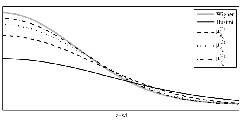
Figure 1: Decay of the Wigner and Husimi function as well as the densities $\mu_{g_{w}}^{N}$, $N\leq 4$, for a Gaussian wave packet $g_{w}$ in dependence of the distance $|z-w|$ from the phase space center.

In higher dimensions one has to incorporate different prefactors and sum over all Hermite spectrograms of the same total degree, but the structure of the approximations (21) remains the same.

For Gaussian superpositions $\psi=g_{z_{1}}+g_{z_{2}}$ with phase space centers $z_{1},z_{2}\in{\mathbb{R}^{2d}}$, and Hermite functions, $\psi=\varphi_{k}$, the second order density $\mu^{2}_{\psi}$ has been computed in [5, §5] by using ladder operators. The same technique can in principle also be used to compute higher order densities $\mu^{N}_{\psi}$, but will lead to tedious calculations. The structure of the densities for a Gaussian superposition, however, is always of the form

$$\mu^{N}_{g_{z_{1}}+g_{z_{2}}}=\mu^{N}_{g_{z_{1}}}+\mu^{N}_{g_{z_{2}}}+{\rm e}^{-|z_{1}-z_{2}|/8{\varepsilon}}C^{N}_{z_{1},z_{2}},$$

where $C^{N}_{z_{1},z_{2}}$ is an oscillatory cross term, see also [5, §5]. The damping factor ${\rm e}^{-|z_{1}-z_{2}|/8{\varepsilon}}$ is exponentially small in ${\varepsilon}$, such that one can safely ignore the cross term in computations as soon as $z_{1}$ and $z_{2}$ are sufficiently apart. In contrast, the cross term in the Wigner function of a Gaussian superposition does not contain a damping factor. Hence, the interferences are large and cannot be neglected.

In this paper we do not further investigate explicit formulas for spectrogram densities. Instead, we discuss a Markov Chain method for sampling from spectrogram densities that is tailored to practical applications. In particular, the method can be applied to a wide range of states and circumvents the difficulties of explicitely computing Wigner or Husimi functions, see §3.2.

3 Applications

3.1 Quantum Expectations

In chemistry, the expectation values of Weyl quantized observables are often computed via the Monte Carlo quadrature

$$\left\langle\psi,{\rm op}(a)\psi\right\rangle=\int_{\mathbb{R}^{2d}}a(z){\mathcal{W}}_{\psi}(z){\rm{d}}z\approx\frac{1}{n}\sum_{m=1}^{n}a(z_{m})$$ (22)

where $z_{1},\ldots,z_{n}\sim{\mathcal{W}}_{\psi}$ are distributed with respect to the Wigner function, see [2, 3]. Generically, however, ${\mathcal{W}}_{\psi}$ is not a probability density and direct sampling techniques cannot be applied. Instead of using methods like importance sampling we propose to replace ${\mathcal{W}}_{\psi}$ by a spectrogram density $\mu^{N}_{\psi}$, which is a linear combination of smooth probability densities. That is, we approximate

$$\left\langle\psi,{\rm op}(a)\psi\right\rangle =\int_{\mathbb{R}^{2d}}a(z)\mu^{N}_{\psi}(z){\rm{d}}z+O({\varepsilon}^{N})$$

$$\approx\sum_{j=0}^{N-1}(-1)^{j}C_{N-1,j}{N+d-1\choose d-1}\frac{1}{n}\sum_{m=1}^{n}a(z^{j}_{m}),$$ (23)

where the phase space points are sampled from the probability densities given by the averaged Hermite spectrograms of a given order,

$$z^{j}_{1},\ldots,z^{j}_{n}\sim{N+d-1\choose d-1}^{-1}\sum_{k\in\mathbb{N}^{d},|k|=j}S_{\psi}^{\varphi_{k}},\quad j=1,\ldots N-1.$$ (24)

Obviously, method (23) is typically only practicable if the dimension $d$ is not too large and one does not need to go to a very high order $N$. However, for the majority of applications in physical chemistry this is the case.

Remark 3.

Instead of considering the probability densities (24) it could often be more practicable to sample from each spectrogram $S_{\psi}^{\varphi_{k}}$, $|k|<N$, seperately. Alternatively, sometimes it might be possible to combine all spectrograms that appear with positive or negative prefactors. In that case, one would only need to sample from two probability densities.

3.2 Sampling via Metropolis-Hastings

Evaluating the highly oscillatory integral (1) defining the Wigner function in several dimensions is numerically extremely challenging or — for the majority of systems — simply unfeasible. Together with the sampling problem arising from the fact that Wigner functions may attain negative values, this is a major bottleneck for the applicability of (22). Moreover, often one also cannot explicitely compute the spectrogram densities (24) either. Instead, we propose a Markov chain sampling scheme for spectrograms based on the inner product representation with Hermite functions

$$S^{\varphi_{k}}_{\psi}(z)=(2\pi{\varepsilon})^{-d}|\left\langle\psi,T_{z}\varphi_{k}\right\rangle|^{2},\quad z\in{\mathbb{R}^{2d}},$$ (25)

where the Heisenberg-Weyl operator $T_{z}$ has been defined in (19); see also [5]. This method does not require to determine $S^{\varphi_{k}}_{\psi}$ globally as a function, but only involves pointwise evaluations.

For approximating the inner products (25) one can use different methods. Natural choices certainly include Gauss-Hermite, Monte Carlo or Quasi-Monte Carlo quadrature rules. All these schemes exploit the Gaussian factor appearing in the Hermite functions. Monte Carlo quadrature is especially useful in higher dimensions, where one would need to employ sparse grids when applying Gauss-Hermite quadrature, see, e.g., [25, §III.1].

We propose to generate a Markov chain with stationary distribution $S^{\varphi_{k}}_{\psi}$ via the Metropolis-Hastings algorithm. We implement the following iteration that starts from a seed $z_{0}\in{\mathbb{R}^{2d}}$ with probability $S^{\varphi_{k}}_{\psi}(z_{0})$.

1. Proposition: set $z=z_{n}+\sqrt{{\varepsilon}}\zeta$ with a random vector $\zeta\sim N(0,{\rm Id}_{2d})$.

2. Quadrature: approximately evaluate $S^{\varphi_{k}}_{\psi}(z)$ via (25).

3. Acceptance: generate a uniform random number $\rho\sim U([0,1])$. Accept the trial point if $\rho<S^{\varphi_{k}}_{\psi}(z)/S^{\varphi_{k}}_{\psi}(z_{n})$, and set $z_{n+1}=z$. Otherwise, reject the proposition and keep the old point $z_{n+1}=z_{n}$.

We used a normal density of variance ${\varepsilon}$ as proposal distribution, since — as the Husimi function of a Gaussian wave packet — it is a prototype spectrogram for functions with $O({\varepsilon}^{-1})$ frequencies. If one knows in advance that the spectrogram $S^{\varphi_{k}}_{\psi}$ has a disconnected effective support in phase space, one may additionally incorporate a jump step in the spirit of [26, §5.1].

If the Markov chain $\{z_{n}\}_{n}$ is uniformly ergodic, the central limit theorem implies weak convergence of averages, see [27]. More precisely, for any function $a:{\mathbb{R}^{2d}}\to\mathbb{R}$ that is square-integrable with respect to $S^{\varphi_{k}}_{\psi}$ there is a constant $c_{a}$ such that

$$\lim_{n\to\infty}\mathbb{P}\left(\bigg{|}\tfrac{1}{n}\sum_{j=1}^{n}a(z_{j})-\int_{\mathbb{R}^{2d}}a(z)S^{\varphi_{k}}_{\psi}(z){\rm{d}}z\bigg{|}\leq\frac{rc_{a}}{\sqrt{n}}\right)=\frac{1}{\sqrt{2\pi}}\int_{-r}^{r}{\rm e}^{-t^{2}/2}{\rm{d}}t$$

for any $r>0$. In particular, this implies convergence of the method (23) for the computation of quantum expectation values. We stress that the convergence rate of $n^{-1/2}$ does not depend on the dimension $d$ of the configuration space.

3.3 Quantum dynamics

In physical chemistry, the computation of stationary quantum expectation values itself is not of central interest. Instead, one would like to compute the evolution of expectation values

$$t\mapsto\left\langle\psi_{t},{\rm op}(a)\psi_{t}\right\rangle.$$

where the wave function $\psi_{t}$ represents the state of the molecule’s nuclei at time $t$ in the Born-Oppenheimer approximation. Here, the evolution of the wave function $\psi_{t}$ on an electronic potential energy surface $V$ is typically described by the bona fide Schrödinger equation

$$i{\varepsilon}\partial_{t}\psi_{t}=-\tfrac{{\varepsilon}^{2}}{2}\Delta\psi_{t}+V\psi_{t},$$

where the small parameter $0<{\varepsilon}\ll 1$ represents the square root of the electronic versus average nuclear mass; see [28]. Consequently, by combining Egorov’s theorem (see [8, 3]) with (13) one obtains the second order approximation

$$\left\langle\psi_{t},{\rm op}(a)\psi_{t}\right\rangle =\int_{\mathbb{R}^{2d}}{\mathcal{W}}_{\psi_{0}}(z)(a\circ\Phi^{t})(z){\rm{d}}z+O({\varepsilon}^{2})$$ (26)

$$=\int_{\mathbb{R}^{2d}}\mu^{2}_{\psi_{0}}(z)a(z){\rm{d}}z+O({\varepsilon}^{2}),$$ (27)

where $\Phi^{t}$ is the the flow of the underlying classical Hamiltonian system $\dot{q}=p$, $\dot{p}=-\nabla V(q)$. This approximation and its discretization has been studied in [5].

The spectrogram method (27) improves the Wigner function method (26) that has been widely used in chemical physics since decades under the name linearized semiclassical initial value representation (LSC-IVR) or Wigner phase space method; see, e.g., [2, 3].

One can construct higher order versions of (27) that only require sampling from probability densities and solving ordinary equations. For this purpose one combines the densities $\mu^{N}_{\psi_{0}}$ from Theorem 1 with higher order corrections of Egorov’s theorem for the quantum dynamics, see [8, 7]. We leave the details to future investigations.

4 Numerical Experiments

4.1 Accuracy

In a first set of experiments we investigate if the asymptotic error of our approximation from Theorem 1 is observed in practice. For this purpose we consider a one-dimensional Gaussian wave packet $\psi=g_{z_{0}}$ centered in $z_{0}=(\tfrac{1}{2},-1)$ and varying values of ${\varepsilon}$. We compare the expectation values of the following observables with their approximation via the spectrogram approximation with density $\mu_{\psi}^{N}$ for the orders $N=1,\ldots,4$:

1. $a(q,p)=q^{4}+1$

2. $b(q,p)=\tfrac{1}{4}(p^{2}-q)^{3}$

3. $c(q,p)=\cos(q)$

4. $d(q,p)=\exp(\sin(q))$.

We used the formulas for the spectrogram densities $\mu_{\psi}^{N}$ from (21). For the observables $a$, $b$ and $c$ all computations can be done explicitely. For the observable $d$ we used a highly accurate quadrature scheme. The results depicted in figure 2 show that the errors are indeed of order $O({\varepsilon}^{N})$. Moreover, as expected, in the cases $N=3$ and $N=4$ the observables $a$ respectively $a$ and $b$ are reproduced without error.

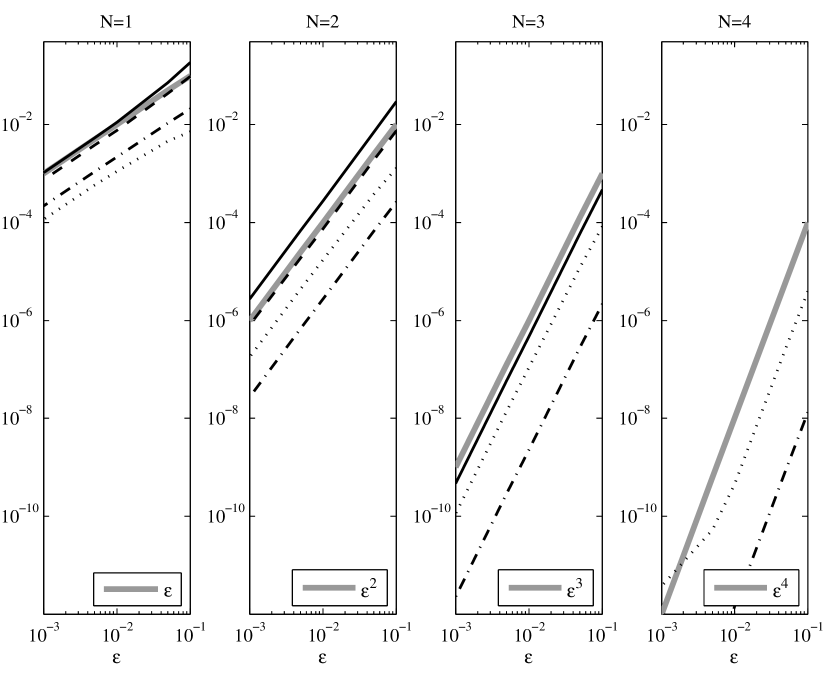
Figure 2: Errors of the expectation values of the observables $a$ (dashed), $b$ (solid), $c$ (dashed dotted) and $d$ (dotted) computed by the spectrogram approximations of order $N\in\{1\ldots 4\}$. The state is a Gaussian wave packet centered in $(\tfrac{1}{2},-1)$.

We highlight that the error constants do not seem to grow with the order, although $\mu^{N}_{\psi}$ only weakly approximates ${\mathcal{W}}_{\psi}$. This indicates that stronger types of convergence might hold for particular states and observables.

4.2 Sampling a hat function

In a second set of experiments we consider the normalized semiclassical hat function

$$\psi(x)=\sqrt{\tfrac{3}{2\sqrt{{\varepsilon}}}}\left(1-\frac{|x-q|}{\sqrt{\varepsilon}}\right)1_{|x-q|<\sqrt{{\varepsilon}}},\quad x\in\mathbb{R},$$ (28)

that is localized around $q\in\mathbb{R}$. Computing the Wigner functions and spectrograms of $\psi$ explicitely is difficult. Therefore, we sample from the densities $\mu_{\psi}^{N}$ by means of the Markov chain Monte Carlo algorithm introduced in §3.2, and discretize the inner prduct (25) by Quasi-Monte Carlo quadrature with $10^{3}$ Sobol points.

In figure 3 one can see that the numerically computed Wigner function and its approximative reconstruction via the weighted histogram

$$z\mapsto\frac{1}{n}\sum_{j=0}^{2}(-1)^{j}C_{2,j}\#\{k:z^{j}_{k}\approx z\},\quad z^{j}_{1},\ldots,z^{j}_{n}\sim S_{\psi}^{\varphi_{j}}$$ (29)

of the signed density $\mu^{3}_{\psi}$ look very similar. In fact, the weighted histogram attains negative values in the same regions where also the Wigner functions becomes negative.

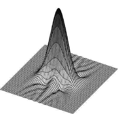
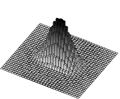
Figure 3: The Wigner function of the hat function (28) and a weighted histogram reconstruction (29) of the spectrogram density $\mu^{3}_{\psi}$ with $10^{6}$ samples, where ${\varepsilon}=5\cdot 10^{-2}$.

In order to investigate the applicability of the Markov chain sampling algorithm from §3.2 we now explore the errors for observables in dependence of the chosen number of Monte Carlo points. We consider the expectations of the position observable $a(q,p)=q$, that is, the center of the sampled distribution, as well as of the complicated observable $d$ from the previous section. We consider samplings of both a single Husimi function and the second order spectrogram density $\mu_{\psi}^{2}$ for the fixed parameter ${\varepsilon}=10^{-2}$.

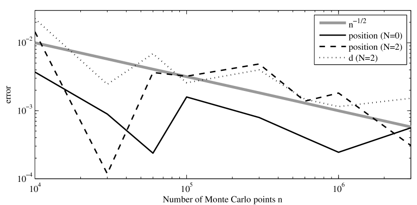
Figure 4: Errors for the sampling method from §3.2 in dependence of the used Monte Carlo points for the position in the case $N=0$, the position in the case $N=2$, and the observable $d$ in the case $N=2$. The results are averaged over ten independent runs.

Figure 4 illustrates that, as expected, the asymptotic sampling error of order $O(n^{-1/2})$ for Markov chain Monte Carlo methods is also observed for our algorithm, although the probability densities are only approximately evaluated via quadrature. We note that it is necessary to use a sufficiently accurate quadrature in order to observe decent convergence results.

Our experiments confirm that the Markov chain method from §3.2 is applicable for the approximative sampling of Wigner functions in the semiclassical regime. The method could prove particularly useful in higher dimensions, where Wigner functions typically cannot be computed.

Appendix A Proof of Proposition 1

Proof of Proposition 1.

We prove the assertion by induction. Since $L_{0}\equiv 1$, the base case $N=0$ is clear and we assume that the assertion is true for some $N\in\mathbb{N}$. We compute

$$\nabla{\mathcal{W}}_{g_{0}}(z) =-\tfrac{2}{{\varepsilon}}z{\mathcal{W}}_{g_{0}}(z) \nabla L_{n}(\varrho(z)) =\tfrac{4}{{\varepsilon}}zL_{n}^{\prime}(\varrho(z))$$

$$\Delta{\mathcal{W}}_{g_{0}}(z) =\tfrac{4}{{\varepsilon}}(\tfrac{\varrho(z)}{2}-1){\mathcal{W}}_{g_{0}}(z) \Delta L_{n}(\varrho(z)) =\tfrac{4}{{\varepsilon}}\left(2L_{n}^{\prime}(\varrho(z))+2\varrho(z)L^{\prime\prime}_{n}(\varrho(z))\right),$$

and from now on write $\varrho(z)=\varrho$ for simplicity. One has

$$\tfrac{{\varepsilon}}{2} \Delta({\mathcal{W}}_{g_{0}}(z)L_{n}(\varrho))={\mathcal{W}}_{g_{0}}(z)\,\left[\,L_{n}(\varrho)(\varrho-2)+4L_{n}^{\prime}(\varrho)+4\varrho L_{n}^{\prime\prime}(\varrho)-4\varrho L_{n}^{\prime}(\varrho)\,\right]\,$$

$$=-{\mathcal{W}}_{g_{0}}(z)\,\left[\,L_{n}(\varrho)(2-\varrho)-4L_{n}^{\prime}(\varrho)-4\varrho L_{n}^{\prime\prime}(\varrho)+4\varrho L_{n}^{\prime}(\varrho)\,\right]\,$$ (30)

and, hence, the polynomial factor in (30) can be rewritten as

$$L_{n}(\varrho)(2-\varrho) -4\varrho L_{n}^{\prime\prime}(\varrho)+4(\varrho-1)L_{n}^{\prime}(\varrho)=L_{n}(\varrho)(2-\varrho+4n)$$

$$=L_{n}(\varrho)(1+2n)+(n+1)L_{n+1}(\varrho)+nL_{n-1}(\varrho).$$ (31)

For verifying (31) one combines Laguerre’s differential equation

$$xL_{n}^{\prime\prime}(x)=(x-1)L_{n}^{\prime}(x)-nL_{n}(x),$$

and the three-term recurrence relation

$$(n+1)L_{n+1}(x)=(2n+1-x)L_{n}(x)-nL_{n-1}(x),\quad n\in\mathbb{N},$$

where $L_{0}\equiv 1$ and $L_{-1}\equiv 0$. Consequently, by the induction hypothesis and (31),

$$\left(-\tfrac{{\varepsilon}}{2}\Delta\right)^{N+1}{\mathcal{W}}_{g_{0}}(z)=N!\sum_{n=0}^{N}{N\choose n}\left(-\tfrac{{\varepsilon}}{2}\Delta\right)({\mathcal{W}}_{g_{0}}(z)L_{n}(\varrho))$$

$$=N!{\mathcal{W}}_{g_{0}}(z)\sum_{n=0}^{N}{N\choose n}\,\left[\,L_{n}(\varrho)(1+2n)+(n+1)L_{n+1}(\varrho)+nL_{n-1}(\varrho)\,\right]\,$$ (32)

and we have to count the prefactors of the polynomials $L_{n}(\varrho)$ for $n=0,\ldots,N+1$ in the sum. For $L_{N+1}(\varrho)$ we have the prefactor

$$(N+1)L_{N+1}(\varrho)=(N+1){N+1\choose N+1}L_{N+1}(\varrho)$$

from the $N$th summand in (32). For $L_{N}(\varrho)$ we get contributions from the $N$th and the $(N-1)$th summand, and observe

$$\left((1+2N)+N{N\choose N-1}\right)L_{N}(\varrho)=(N+1){N+1\choose N}L_{N}(\varrho).$$

For all $1\leq n\leq N-1$ we get contributions from the $n$th, the $(n+1)$th, and the $(n-1)$th summand. Combining them yields

$$\left({N\choose n-1}n+{N\choose n}(1+2n)+{N\choose n+1}(n+1)\right)L_{n}(\varrho)$$

$$=\left(n{N+1\choose n}+(n+1){N+1\choose n+1}\right)L_{n}(\varrho)=(N+1){N+1\choose n}L_{n}(\varrho),$$

and for $L_{0}$ we again have the prefactor $(N+1)$. Finally, rewriting (32) as a sum over $L_{n}(\varrho)$ with $n=0,\ldots,N+1$ completes the proof. ∎

Appendix B Binomial identities

We summarize some binomial identities we repeatedly employ in our proofs. By applying Pascal’s identity multiple times one directly obtains the formula

$$\sum_{j=0}^{N}{k+j\choose j} ={k+N+1\choose N}.$$ (33)

Furthermore, for all $N,m,k\in N$ one has

$$\sum_{j=0}^{N}{N+m-j\choose m}{k+j\choose j}={N+m+k+1\choose N}.$$ (34)

For the proof of (34) we use generating functions, and set

$$a_{N}={N+m\choose N},\quad b_{N}={N+k\choose N},\quad c_{N}:=\sum_{j=0}^{N}{N+m-j\choose m}{k+j\choose j}$$

such that

$$\sum_{j\geq 0}a_{j}x^{j}=(1-x)^{-(m+1)},\quad\sum_{j\geq 0}b_{j}x^{j}=(1-x)^{-(k+1)}$$ (35)

for all $|x|<1$. Then, $c_{N}$ is the $N$th term in the Cauchy product of $(a_{j})_{j\geq 0}$ and $(b_{j})_{j\geq 0}$, and hence

$$\sum_{j\geq 0}c_{j}x^{j}=(1-x)^{-(m+k+2)}.$$

Comparing the coefficients with the power series (35) implies the assertion.

References

• [1] M. A. de Gosson, Symplectic methods in harmonic analysis and in mathematical physics, Vol. 7 of Pseudo-Differential Operators. Theory and Applications, Birkhäuser/Springer Basel AG, Basel, 2011.
• [2] M. Thoss, H. Wang, Semiclassical description of molecular dynamics based on initial-value representation methods, Ann. Rev. Phys. Chem. 55 (1) (2004) 299–332.
• [3] J. Keller, C. Lasser, Quasi-classical description of molecular dynamics based on Egorov’s theorem, J. Chem. Phys. 141 (5) (2014) 054104.
• [4] J. Keller, C. Lasser, Propagation of quantum expectations with Husimi functions, SIAM Journal on Applied Mathematics 73 (4) (2013) 1557–1581.
• [5] J. Keller, C. Lasser, T. Ohsawa, A New Phase Space Density for Quantum Expectations, SIAM J. Math. Anal. 48 (1) (2016) 513–537.
• [6] J. Keller, Quantum Dynamics on Potential Energy Surfaces — Simpler States and Simpler Dynamics, Ph.D. thesis, Technische Universität München (2015).
• [7] W. Gaim, C. Lasser, Corrections to Wigner type phase space methods, Nonlinearity 27 (2014) 2951–2974.
• [8] A. Bouzouina, D. Robert, Uniform semiclassical estimates for the propagation of quantum observables, Duke Math. J. 111 (2002) 223–252.
• [9] F. Auger, P. Flandrin, Y. T. Lin, S. McLaughlin, S. Meignen, T. Oberlin, H. T. Wu, Time-frequency reassignment and synchrosqueezing: An overview, IEEE Signal Processing Magazine 30 (6) (2013) 32–41.
• [10] P. Flandrin, Frequency filtering based on spectrogram zeros, Signal Processing Letters, IEEE 22 (11) (2015) 2137–2141.
• [11] P. Loughlin, J. Pitton, B. Hannaford, Approximating time-frequency density functions via optimal combinations of spectrograms, Signal Processing Letters, IEEE 1 (12) (1994) 199–202.
• [12] A. G. Athanassoulis, N. J. Mauser, T. Paul, Coarse-scale representations and smoothed Wigner transforms, J. Math. Pures Appl. (9) 91 (3) (2009) 296–338.
• [13] W. P. Schleich, Quantum optics in phase space, John Wiley & Sons, 2011.
• [14] G. B. Folland, Harmonic analysis in phase space, Vol. 122 of Annals of Mathematics Studies, Princeton University Press, Princeton, NJ, 1989.
• [15] F. Soto, P. Claverie, When is the Wigner function of multidimensional systems nonnegative?, J. Math. Phys. 24 (1) (1983) 97–100.
• [16] A. J. E. M. Janssen, Positivity and spread of bilinear time-frequency distributions, in: The Wigner distribution, Elsevier, Amsterdam, 1997, pp. 1–58.
• [17] P. Flandrin, A note on reassigned Gabor spectrograms of Hermite functions, J. Fourier Anal. Appl. 19 (2) (2013) 285–295.
• [18] P. Flandrin, Time-frequency/time-scale analysis, Vol. 10 of Wavelet Analysis and its Applications, Academic Press, Inc., San Diego, CA, 1999, with a preface by Yves Meyer, Translated from the French by Joachim Stöckler.
• [19] K. Husimi, Some Formal Properties of the Density Matrix, Nippon Sugaku-Buturigakkwai Kizi Dai 3 Ki 22 (4) (1940) 264–314.
• [20] S. Thangavelu, Lectures on Hermite and Laguerre Expansions, Mathematical Notes - Princeton University Press, Princeton University Press, 1993.
• [21] N. Lerner, Metrics on the phase space and non-selfadjoint pseudo-differential operators, Vol. 3 of Pseudo-Differential Operators. Theory and Applications, Birkhäuser Verlag, Basel, 2010.
• [22] M. Zworski, Semiclassical analysis, Vol. 138 of Graduate Studies in Mathematics, American Mathematical Society, Providence, RI, 2012.
• [23] G. Szegö, Orthogonal polynomials, 4th Edition, American Mathematical Society, Providence, R.I., 1975, american Mathematical Society, Colloquium Publications, Vol. XXIII.
• [24] C. Lasser, S. Troppmann, Hagedorn wavepackets in time-frequency and phase space, J. Fourier An. Appl. (2014) 1–36.
• [25] C. Lubich, From quantum to classical molecular dynamics: reduced models and numerical analysis, Zurich Lectures in Advanced Mathematics, European Mathematical Society (EMS), Zürich, 2008.
• [26] S. Kube, C. Lasser, M. Weber, J. Comput. Phys. 228 (6) (2009) 1947–1962.
• [27] L. Tierney, Markov chains for exploring posterior distributions, Ann. Statist. 22 (4) (1994) 1701–1762, with discussion and a rejoinder by the author.
• [28] H. Spohn, S. Teufel, Adiabatic decoupling and time-dependent Born-Oppenheimer theory, Comm. Math. Phys. 224 (1) (2001) 113–132, dedicated to Joel L. Lebowitz.