A scaled Bregman theorem with applications

Abstract

Bregman divergences play a central role in the design and analysis of a range of machine learning algorithms. This paper explores the use of Bregman divergences to establish reductions between such algorithms and their analyses. We present a new scaled isodistortion theorem involving Bregman divergences (scaled Bregman theorem for short) which shows that certain “Bregman distortions” (employing a potentially non-convex generator) may be exactly re-written as a scaled Bregman divergence computed over transformed data. Admissible distortions include geodesic distances on curved manifolds and projections or gauge-normalisation, while admissible data include scalars, vectors and matrices.

Our theorem allows one to leverage to the wealth and convenience of Bregman divergences when analysing algorithms relying on the aforementioned Bregman distortions. We illustrate this with three novel applications of our theorem: a reduction from multi-class density ratio to class-probability estimation, a new adaptive projection free yet norm-enforcing dual norm mirror descent algorithm, and a reduction from clustering on flat manifolds to clustering on curved manifolds. Experiments on each of these domains validate the analyses and suggest that the scaled Bregman theorem might be a worthy addition to the popular handful of Bregman divergence properties that have been pervasive in machine learning.

1 Introduction: Bregman divergences as a reduction tool

Bregman divergences play a central role in the design and analysis of a range of machine learning algorithms. In recent years, Bregman divergences have arisen in procedures for convex optimisation [Beck and Teboulle, 2003], online learning [Cesa-Bianchi and Lugosi, 2006, Chapter 11] clustering [Banerjee et al., 2005], matrix approximation [Dhillon and Tropp, 2008], class-probability estimation [Buja et al., 2005, Nock and Nielsen, 2009, Reid and Williamson, 2010, 2011], density ratio estimation [Sugiyama et al., 2012], boosting [Collins et al., 2002], variational inference [Hernández-Lobato et al., 2016], and computational geometry [Boissonnat et al., 2010]. Despite these being very different applications, many of these algorithms and their analyses basically rely on three beautiful analytic properties of Bregman divergences, properties that we summarize for differentiable scalar convex functions $\varphi$ with derivative $\varphi^{\prime}$, conjugate $\varphi^{\star}$, and divergence $D_{\varphi}$:

• the triangle equality: $D_{\varphi}(x\|y)+D_{\varphi}(y\|z)-D_{\varphi}(x\|z)=(\varphi^{\prime}(z)-\varphi^{\prime}(y))(x-y)$;

• the dual symmetry property: $D_{\varphi}(x\|y)=D_{\varphi^{\star}}(\varphi^{\prime}(y)\|\varphi^{\prime}(x))$;

• the right-centroid (population minimizer) is the average: $\arg\min_{\mu}\mathbb{E}[D_{\varphi}(\mathsf{X}\|\mu)]=\mathbb{E}[\mathsf{X}]$.

Casting a problem as a Bregman minimisation allows one to employ these properties to simplify analysis; for example, by interpreting mirror descent as applying a particular Bregman regulariser, Beck and Teboulle [2003] relied on the triangle equality above to simplify its proof of convergence.

Another intriguing possibility is that one may derive reductions amongst learning problems by connecting their underlying Bregman minimisations. Menon and Ong [2016] recently established how (binary) density ratio estimation (DRE) can be exactly reduced to class-probability estimation (CPE). This was facilitated by interpreting CPE as a Bregman minimisation [Buja et al., 2005, Section 19], and a new property of Bregman divergences — Menon and Ong [2016, Lemma 2] showed that for any twice differentiable scalar convex $\varphi$, for $g(x)=1+x$ and $\varphi^{\dagger}(x)\stackrel{{\scriptstyle\mathrm{.}}}{{=}}g(x)\cdot\varphi(x/g(x))$,

$$g(x)\cdot D_{\varphi}(x/g(x)\|y/g(y))=D_{\varphi^{\dagger}}(x\|y).$$ (1)

Since the binary class-probability function $\eta(\bm{x})=\Pr(\mathsf{Y}=1|\mathsf{X}=\bm{x})$ is related to the class-conditional density ratio $r(\bm{x})=\Pr(\mathsf{X}=\bm{x}|\mathsf{Y}=1)/\Pr(\mathsf{X}=\bm{x}|\mathsf{Y}=-1)$ via Bayes’ rule as $\eta(\bm{x})=r(\bm{x})/g(r(\bm{x}))$, any $\hat{\eta}$ with small $D_{\varphi}(\eta\|\hat{\eta})$ implicitly produces an $\hat{r}$ with low $D_{\varphi^{\dagger}}(r\|\hat{r})$ i.e. a good estimate of the density ratio. The Bregman property of Equation 1 thus establishes a reduction from DRE to CPE. Two natural questions arise from this analysis: can we generalise Equation 1 to other $g(\cdot)$, and if so, can we similarly relate other problems to each other?

This paper presents a new Bregman identity (Theorem 1), the scaled Bregman theorem, a significant generalisation of Menon and Ong [2016, Lemma 2]. It shows that general distortions $D_{\varphi^{\dagger}}$ – which are not necessarily convex, positive, bounded or symmetric – may be re-expressed as a Bregman divergence $D_{\varphi}$ computed over transformed data, where this transformation can be as simple as a projection or normalisation by a gauge, or more involved like the exponential map on lifted coordinates for a curved manifold. Interestingly, candidate distortions include geodesic distances on curved manifolds. Equivalently, Theorem 1 shows various distortions can be “reverse engineered” as Bregman divergences (despite appearing prima facie to be a very different object), and thus inherit their good properties. Hence, Bregman divergences can embed several distances in a different — and arguably less involved — way than the transformations known to date [Acharyya et al., 2013].

As with the aforementioned key properties of Bregman divergences, Theorem 1 has potentially wide applicability. We present three such novel applications (see Table 1) to vastly different problems:

• a reduction of multiple density ratio estimation to multiclass-probability estimation (§3), generalising the results of Menon and Ong [2016] for the binary label case,

• a projection-free yet norm-enforcing mirror gradient algorithm (enforced norms are those of mirrored vectors and of the offset) with guarantees for adaptive filtering (§4), and

• a seeding approach for clustering on positively or negatively (constant) curved manifolds based on a popular seeding for flat manifolds and with the same approximation guarantees (§5).

Experiments on each of these domains (§6) validate our analysis. The Supplementary Material details the proofs of all results, provides the experimental results in extenso and some additional (nascent) applications of the scaled Bregman theorem to exponential families and computational geometry.

Problem A	Problem B that Theorem 1 reduces A to	Reference
Multiclass density-ratio estimation	Multiclass class-probability estimation	§3, Lemma 2
Online optimisation on $L_{q}$ ball	Convex unconstrained online learning	§4, Lemma 4
Clustering on curved manifolds	Clustering on flat manifolds	§5, Lemma 5

Table 1: Applications of our scaled Bregman Theorem (Theorem 1) — “Reduction” encompasses shortcuts on algorithms and on analyses (algorithm/proof A uses algorithm/proof B as subroutine).

2 Main result: the scaled Bregman theorem

In the remaining, $[k]\stackrel{{\scriptstyle\mathrm{.}}}{{=}}\{0,1,...,k\}$ and $[k]_{*}\stackrel{{\scriptstyle\mathrm{.}}}{{=}}\{1,2,...,k\}$ for $k\in\mathbb{N}$. For any differentiable (but not necessarily convex) $\varphi:{\mathcal{X}}\rightarrow{\mathbb{R}}$, we define the Bregman “distortion” $D_{\varphi}$ as

$$D_{\varphi}(\bm{x}\|\bm{y}) \stackrel{{\scriptstyle\mathrm{.}}}{{=}} \varphi(\bm{x})-\varphi(\bm{y})-(\bm{x}-\bm{y})^{\top}\nabla\varphi(\bm{y})\>\>.$$ (2)

When $\varphi$ is convex, $D_{\varphi}$ is the familiar Bregman divergence with generator $\varphi$.

Without further ado, we present our main result.

Theorem 1

Let, $\varphi:{\mathcal{X}}\rightarrow{\mathbb{R}}$ be convex differentiable, and $g:{\mathcal{X}}\rightarrow{\mathbb{R}}_{*}$ be differentiable. Then,

$$g(\bm{x})\cdot D_{\varphi}\left(\bm{x}/g(\bm{x})\bigm{\|}\bm{y}/g(\bm{y})\right) = D_{\varphi^{\dagger}}\left(\bm{x}\bigm{\|}\bm{y}\right)\>\>,\forall\bm{x},\bm{y}\in\mathcal{X}\>\>,$$ (3)

$$\text{ where }\varphi^{\dagger}(\bm{x}) \stackrel{{\scriptstyle\mathrm{.}}}{{=}} g(\bm{x})\cdot\varphi\left(\bm{x}/{g(\bm{x})}\right)\>\>,$$ (4)

if and only if (i) $g$ is affine on $\mathcal{X}$, and/or (ii) for every $\bm{z}\in\mathcal{X}_{g}\stackrel{{\scriptstyle\mathrm{.}}}{{=}}\{(1/g(\bm{x}))\cdot\bm{x}:\bm{x}\in\mathcal{X}\}$,

$$\varphi\left(\bm{z}\right)=\bm{z}^{\top}\nabla\varphi(\bm{z})\>\>.$$ (5)

Table 2 presents some examples of (sometimes involved) triplets $(D_{\varphi},D_{\varphi^{\dagger}},g)$ for which Equation 3 holds; related proofs are in Appendix C. If we fold $g$ into $D_{\varphi}$ in the left hand-side of eq. (3), then Theorem 1 states a scaled isodistortion (sometimes it turns out to be equivalently an adaptive scaled isometry, see Appendix I) property between $\mathcal{X}$ and $\mathcal{X}_{g}$. Because $D_{\varphi}$ is such an important object, we do not perform this folding and refer to Theorem 1 as the scaled Bregman theorem for short.

Remark.  If $\mathcal{X}_{g}$ is a vector space, $\varphi$ satisfies Equation 5 if and only if it is positive homogeneous of degree 1 on $\mathcal{X}_{g}$ (i.e. $\varphi(\alpha\bm{z})=\alpha\cdot\varphi(\bm{z})$ for any $\alpha>0$) from Euler’s homogenous function theorem. When $\mathcal{X}_{g}$ is not a vector space, this only holds for $\alpha$ such that $\alpha\bm{z}\in\mathcal{X}_{g}$ as well. We thus call the gradient condition of Equation 5 “restricted positive homogeneity” for simplicity.  

Remark.  Appendix D gives a “deep composition” extension of Theorem 1.  

For the special case where $\mathcal{X}=\mathbb{R}$, and $g(x)=1+x$, Theorem 1 is exactly Menon and Ong [2016, Lemma 2] (c.f. Equation 1). We wish to highlight a few points with regard to our more general result. First, the “distortion” generator $\varphi^{\dagger}$ may be non-convex, as the following illustrates.

Example.  Suppose $\varphi(\bm{x})=\frac{1}{2}\|\bm{x}\|_{2}^{2}$ corresponds to the generator for squared Euclidean distance. Then, for $g(\bm{x})=1+\bm{1}^{\top}\bm{x}$, we have $\varphi^{\dagger}(\bm{x})=\frac{1}{2}\cdot\frac{\|\bm{x}\|_{2}^{2}}{1+\bm{1}^{\top}\bm{x}},$ which is non-convex on $\mathcal{X}=\mathbb{R}^{d}$.  

When $\varphi^{\dagger}$ is non-convex, the right hand side in Equation 3 is an object that ostensibly bears only a superficial similarity to a Bregman divergence; it is somewhat remarkable that Theorem 1 shows this general “distortion” between a pair $(\bm{x},\bm{y})$ to be entirely equivalent to a (scaling of a) Bregman divergence between some transformation of the points. Second, when $g$ is linear, Equation 3 holds for any convex $\varphi$. (This was the case considered in Menon and Ong [2016].) When $g$ is non-linear, however, $\varphi$ must be chosen carefully so that $(\varphi,g)$ satisfies the restricted homogeneity conditon of Equation 5. In general, given a convex $\varphi$, one can “reverse engineer” a suitable $g$ to guarantee this conditon, as illustrated by the following example.

Example.  Suppose $\varphi(\bm{x})=(1+\|\bm{x}\|_{2}^{2})/2$. Then, Equation 5 requires that $\|\bm{x}\|_{2}^{2}=1$ for every $\bm{x}\in\mathcal{X}_{g}$, i.e. $\mathcal{X}_{g}$ is (a subset of) the unit sphere. This is afforded by the choice $g(\bm{x})=\|\bm{x}\|_{2}$.  

$\mathcal{X}$	$D_{\varphi}\left(\bm{x}\|\bm{y}\right)$	$D_{\varphi^{\dagger}}\left(\bm{x}\|\bm{y}\right)$	$g(\bm{x})$
$\mathbb{R}^{d}$	$\frac{1}{2}\cdot\|\bm{x}-\bm{y}\|_{2}^{2}$	$\|\bm{x}\|_{2}\cdot\left(1-\cos\angle\bm{x},\bm{y}\right)$	$\|\bm{x}\|_{2}$
$\mathbb{R}^{d}$	$\frac{1}{2}\cdot(\|\bm{x}\|_{q}^{2}-\|\bm{y}\|_{q}^{2})-\sum_{i}\frac{(x_{i}-y_{i})\cdot\mathrm{sign}(y_{i})\cdot|y_{i}|^{q-1}}{\|\bm{y}\|_{q}^{q-2}}$	$W\cdot\|\bm{x}\|_{q}-W\cdot\sum_{i}\frac{x_{i}\cdot\mathrm{sign}(y_{i})\cdot|y_{i}|^{q-1}}{\|\bm{y}\|_{q}^{q-1}}$	$\|\bm{x}\|_{q}/W$
$\mathbb{R}^{d}\times\mathbb{R}$	$\frac{1}{2}\cdot\|\bm{x}^{S}-\bm{y}^{S}\|_{2}^{2}$	$\frac{\|\bm{x}\|_{2}}{\sin\|\bm{x}\|_{2}}\cdot\left(1-\cos D_{G}(\bm{x},\bm{y})\right)$	$\|\bm{x}\|_{2}/\sin\|\bm{x}\|_{2}$
$\mathbb{R}^{d}\times\mathbb{C}$	$\frac{1}{2}\cdot\|\bm{x}^{H}-\bm{y}^{H}\|_{2}^{2}$	$-\frac{\|\bm{x}\|_{2}}{\sinh\|\bm{x}\|_{2}}\cdot\left(\cosh D_{G}(\bm{x},\bm{y})-1\right)$	$-\|\bm{x}\|_{2}/\sinh\|\bm{x}\|_{2}$
$\mathbb{R}_{+}^{d}$	$\sum_{i}x_{i}\log\frac{x_{i}}{y_{i}}-\bm{1}^{\top}(\bm{x}-\bm{y})$	$\sum_{i}x_{i}\log\frac{x_{i}}{y_{i}}-d\cdot\mathbb{E}[\mathsf{X}]\cdot\log\frac{\mathbb{E}[\mathsf{X}]}{\mathbb{E}[\mathsf{Y}]}$	$\bm{1}^{\top}\bm{x}$
$\mathbb{R}_{+}^{d}$	$\sum_{i}\frac{x_{i}}{y_{i}}-\sum_{i}\log\frac{x_{i}}{y_{i}}-d$	$\sum_{i}\frac{x_{i}(\prod_{j}y_{j})^{1/d}}{y_{i}}-d(\prod_{j}x_{j})^{1/d}$	$\prod_{i}x_{i}^{1/d}$
$\textbf{S}(d)$	$\mathrm{tr}\left(\mbox{{\small{x}}}\log\mbox{{\small{x}}}-\mbox{{\small{x}}}\log\mbox{{\small{y}}}\right)-\mathrm{tr}\left(\mbox{{\small{x}}}\right)+\mathrm{tr}\left(\mbox{{\small{y}}}\right)$	$\mathrm{tr}\left(\mbox{{\small{x}}}\log\mbox{{\small{x}}}-\mbox{{\small{x}}}\log\mbox{{\small{y}}}\right)-\mathrm{tr}\left(\mbox{{\small{x}}}\right)\cdot\log\frac{\mathrm{tr}\left(\mbox{{\small{x}}}\right)}{\mathrm{tr}\left(\mbox{{\small{y}}}\right)}$	$\mathrm{tr}\left(\mbox{{\small{x}}}\right)$
$\textbf{S}(d)$	$\mathrm{tr}\left(\mbox{{\small{x}}}\mbox{{\small{y}}}^{-1}\right)-\log\det(\mbox{{\small{x}}}\mbox{{\small{y}}}^{-1})-d$	$\det(\mbox{{\small{y}}}^{1/d})\mathrm{tr}\left(\mbox{{\small{x}}}\mbox{{\small{y}}}^{-1}\right)-d\cdot\det(\mbox{{\small{x}}}^{1/d})$	$\det(\mbox{{\small{x}}}^{1/d})$

Table 2: Examples of $(D_{\varphi},D_{\varphi^{\dagger}},g)$ for which Equation 3 holds. Function $\bm{x}^{S}\stackrel{{\scriptstyle\mathrm{.}}}{{=}}f(\bm{x}):{\mathbb{R}}^{d}\rightarrow{\mathbb{R}}^{d+1}$ and $\bm{x}^{H}\stackrel{{\scriptstyle\mathrm{.}}}{{=}}f(\bm{x}):{\mathbb{R}}^{d}\rightarrow{\mathbb{R}}^{d}\times\mathbb{C}$ are the Sphere and Hyperbolic lifting maps defined in Equation 69, 80. $W>0$ is a constant. $D_{G}$ denotes the $G$eodesic distance on the sphere (for $\bm{x}^{S}$) or the hyperboloid (for $\bm{x}^{H}$). $\textbf{S}(d)$ is the set of symmetric real matrices. Related proofs are in Section C.

Third, Theorem 1 is not merely a mathematical curiosity: we now show that it facilitates novel results in three very different domains, namely estimating multiclass density ratios, constrained online optimisation, and clustering data on a manifold with non-zero curvature. We discuss nascent applications to exponential families and computational geometry in Appendices E and F.

3 Multiclass density-ratio estimation via class-probability estimation

Given samples from a number of densities, density ratio estimation concerns estimating the ratio between each density and some reference density. This has applications in the covariate shift problem wherein the train and test distributions over instances differ [Shimodaira, 2000]. Our first application of Theorem 1 is to show how density ratio estimation can be reduced to class-probability estimation [Buja et al., 2005, Reid and Williamson, 2010].

To proceed, we fix notation. For some integer $C\geq 1$, consider a distribution $\mathbb{P}(\mathsf{X},\mathsf{Y})$ over an (instance, label) space $\mathcal{X}\times[C]$. Let $(\{P_{c}\}_{c=1}^{C},\bm{\pi})$ be densities giving $\mathbb{P}(\mathsf{X}|\mathsf{Y}=c)$ and $\mathbb{P}(\mathsf{Y}=c)$ respectively, and $M$ giving $\mathbb{P}(\mathsf{X})$ accordingly. Fix $c^{*}\in[C]$ a reference class, and suppose for simplicity that $c^{*}=C$. Let $\tilde{\bm{\pi}}\in\bigtriangleup^{C-1}$ such that $\tilde{\pi}_{c}\stackrel{{\scriptstyle\mathrm{.}}}{{=}}\pi_{c}/(1-\pi_{C})$. Density ratio estimation [Sugiyama et al., 2012] concerns inferring the vector $\bm{r}(\bm{x})\in{\mathbb{R}}^{C-1}$ of density ratios relative to $C$, with $r_{c}(\bm{x})\stackrel{{\scriptstyle\mathrm{.}}}{{=}}{\mathbb{P}(\mathsf{X}=\bm{x}|\mathsf{Y}=c)}/{\mathbb{P}(\mathsf{X}=\bm{x}|\mathsf{Y}=C)}\>\>,$ while class-probability estimation [Buja et al., 2005] concerns inferring the vector $\bm{\eta}(\bm{x})\in{\mathbb{R}}^{C-1}$ of class-probabilities, with $\eta_{c}(\bm{x})\stackrel{{\scriptstyle\mathrm{.}}}{{=}}\mathbb{P}(\mathsf{Y}=c|\mathsf{X}=\bm{x})/\tilde{\pi}_{c}\>\>.$ In both cases, we estimate the respective quantities given an iid sample $\mathsf{S}\sim\mathbb{P}(\mathsf{X},\mathsf{Y})^{N}$.

The genesis of the reduction from density ratio to class-probability estimation is the fact that $\bm{r}(\bm{x})=(\pi_{C}/(1-\pi_{C}))\cdot\bm{\eta}(\bm{x})/\eta_{C}(\bm{x})$. In practice one will only have an estimate $\hat{\bm{\eta}}$, typically derived by minimising a suitable loss on the given $\mathsf{S}$ [Williamson et al., 2014], with a canonical example being multiclass logistic regression. Given $\hat{\bm{\eta}}$, it is natural to estimate the density ratio via:

$$\hat{\bm{r}}(\bm{x}) = \frac{\hat{\bm{\eta}}(\bm{x})}{\hat{{\eta}}_{C}(\bm{x})}\>\>.$$ (6)

While this estimate is intuitive, to establish a formal reduction we must relate the quality of $\hat{\bm{r}}$ to that of $\hat{\bm{\eta}}$. Since the minimisation of a suitable loss for class-probability estimation is equivalent to a Bregman minimisation [Buja et al., 2005, Section 19], [Williamson et al., 2014, Proposition 7], this is however immediate by Theorem 1, as shown below.

Lemma 2

Given a class-probability estimator $\hat{\eta}\colon\mathcal{X}\to[0,1]^{C-1}$, let the density ratio estimator $\hat{r}$ be as per Equation 6. Then for any convex differentiable $\varphi\colon[0,1]^{C-1}\to\mathbb{R}$,

$$\mathbb{E}_{\mathsf{X}\sim M}[D_{\varphi}(\bm{\eta}(\mathsf{X})\|\hat{\bm{\eta}}(\mathsf{X}))] = (1-\pi_{C})\cdot\mathbb{E}_{\mathsf{X}\sim P_{C}}\left[D_{\varphi^{\dagger}}(\bm{r}(\mathsf{X})\|\hat{\bm{r}}(\mathsf{X}))\right]\>\>$$ (7)

where $\varphi^{\dagger}$ is as per Equation 4 with $g(\bm{x})\stackrel{{\scriptstyle\mathrm{.}}}{{=}}{\pi_{C}}/({1-\pi_{C}})+\tilde{\bm{\pi}}^{\top}\bm{x}\>\>.$

Lemma 2 generalises Menon and Ong [2016, Proposition 3], which focussed on the binary case with $\pi=\nicefrac{{1}}{{2}}$. (See Appendix G for a review of that result.) Unpacking the Lemma, the LHS in Equation 7 represents the object minimised by some suitable loss for class-probability estimation. Since $g$ is affine, we can use any convex, differentiable $\varphi$, and so can use any suitable class-probability loss to estimate $\hat{\bm{\eta}}$. Lemma 2 thus implies that producing $\hat{\bm{\eta}}$ by minimising any class-probability loss equivalently produces an $\hat{\bm{r}}$ as per Equation 6 that minimises a Bregman divergence to the true $\bm{r}$. Thus, Theorem 1 provides a reduction from density ratio to multiclass probability estimation.

We now detail two applications where $g(\cdot)$ is no longer affine, and $\varphi$ must be chosen more carefully.

4 Dual norm mirror descent: projection-free online learning on $L_{p}$ balls

A substantial amount of work in the intersection of machine learning and convex optimisation has focused on constrained optimisation within a ball [Shalev-Shwartz et al., 2007, Duchi et al., 2008]. This optimisation is typically via projection operators that can be expensive to compute [Hazan and Kale, 2012, Jaggi, 2013]. We now show that gauge functions can be used as an inexpensive alternative, and that Theorem 1 easily yields guarantees for this procedure in online learning.

We consider the adaptive filtering problem, closely related to the online least squares problem with linear predictors [Cesa-Bianchi and Lugosi, 2006, Chapter 11]. Here, over a sequence of $T$ rounds, we observe some $\bm{x}_{t}\in\mathcal{X}$. We must the predict a target value $\hat{y}_{t}=\bm{w}_{t-1}^{\top}\bm{x}_{t}$ using our current weight vector $\bm{w}_{t-1}$. The true target $y_{t}=\bm{u}^{\top}\bm{x}_{t}+\epsilon_{t}$ is then revealed, where $\epsilon_{t}$ is some unknown noise, and we may update our weight to $\bm{w}_{t}$. Our goal is to minimise the regret of the sequence $\{\bm{w}_{t}\}_{t=0}^{T}$,

$$R(\bm{w}_{1:T}|\bm{u})\stackrel{{\scriptstyle\mathrm{.}}}{{=}}\sum_{t=1}^{T}\left(\bm{u}^{\top}\bm{x}_{t}-\bm{w}_{t-1}^{\top}\bm{x}_{t}\right)^{2}-\sum_{t=1}^{T}\left(\bm{u}^{\top}\bm{x}_{t}-y_{t}\right)^{2}\>\>.$$ (8)

Let $q\in(1,2]$ and $p$ be such that $1/p+1/q=1$. For $\varphi\stackrel{{\scriptstyle\mathrm{.}}}{{=}}\frac{1}{2}\cdot\|\bm{x}\|_{q}^{2}$ and loss $\ell_{t}(\bm{w})=\frac{1}{2}\cdot(y_{t}-\bm{w}^{\top}\bm{x}_{t})^{2}$, the $p$-LMS algorithm [Kivinen et al., 2006] employs the stochastic mirror gradient updates

$$\bm{w}_{t} \stackrel{{\scriptstyle\mathrm{.}}}{{=}} \underset{\bm{w}}{\operatorname{argmin}}\,{\eta_{t}}\cdot\ell_{t}(\bm{w})+D_{\varphi}(\bm{w}\|\bm{w}_{t-1})=(\nabla\varphi)^{-1}\left(\nabla\varphi(\bm{w}_{t-1})-\eta_{t}\cdot\nabla\ell_{t}\right),$$ (9)

where $\eta_{t}$ is a learning rate to be specified by the user. Kivinen et al. [2006, Theorem 2] shows that for appropriate $\eta_{t}$, one has $R(\bm{w}_{1:T}|\bm{u})\leq(p-1)\cdot\max_{\bm{x}\in\mathcal{X}}\|\bm{x}\|_{p}^{2}\cdot\|\bm{u}\|_{q}^{2}$.

The $p$-LMS updates do not provide any explicit control on $\|\bm{w}_{t}\|$, i.e. there is no regularisation. Experiments ($\S$6) suggest that leaving $\|\bm{w}_{t}\|$ uncontrolled may not be a good idea as the increase of the norm sometimes prevents (significant) updates (9). Also, the wide success of regularisation in machine learning calls for regularised variants that retain the regret guarantees and computational efficiency of $p$-LMS. (Adding a projection step to Equation 9 would not achieve both.) We now do just this. For fixed $W>0$, let $\varphi\stackrel{{\scriptstyle\mathrm{.}}}{{=}}(1/2)(W^{2}+\|\bm{x}\|_{q}^{2})$, a translation of that used in $p$-LMS. Invoking Theorem 1 with the admissible $g_{q}(\bm{x})=||\bm{x}||_{q}/W$ yields $\varphi^{\dagger}\stackrel{{\scriptstyle\mathrm{.}}}{{=}}\varphi_{q}^{\dagger}=W\|\bm{x}\|_{q}$ (see Table 2). Using the fact that $L_{p}$ and $L_{q}$ norms are dual of each other, we replace Equation 9 by:

$$\bm{w}_{t} \stackrel{{\scriptstyle\mathrm{.}}}{{=}} \nabla{\varphi_{p}^{\dagger}}\left(\nabla\varphi_{q}^{\dagger}(\bm{w}_{t-1})-\eta_{t}\cdot\nabla\ell_{t}\right)\>\>.$$ (10)

See Lemma 6 of the Appendix for the simple forms of $\nabla\varphi_{\{p,q\}}^{\dagger}$. We call update (10) the dual norm $p$-LMS (DN-pLMS) algorithm, noting that the dual refers to the polar transform of the norm, and $g$ stems from a gauge normalization for ${\mathcal{B}}_{q}(W)$, the closed $L_{q}$ ball with radius $W>0$. Namely, we have $\gamma_{\textsc{gau}}(\bm{x})=W/\|\bm{x}\|_{q}=g(\bm{x})^{-1}$ for the gauge $\gamma_{\textsc{gau}}(\bm{x})\stackrel{{\scriptstyle\mathrm{.}}}{{=}}\sup\{z\geq 0:z\cdot\bm{x}\in{\mathcal{B}}_{q}(W)\}$, so that $\varphi_{q}^{\dagger}$ implicitly performs gauge normalisation of the data. This update is no more computationally expensive than Equation 9 — we simply need to compute the $p$- and $q$-norms of appropriate terms — but, crucially, automatically constrains the norms of $\bm{w}_{t}$ and its image by $\nabla{\varphi_{q}^{\dagger}}$.

Lemma 3

For the update in Equation 10, $\|\bm{w}_{t}\|_{q}=\|\nabla{\varphi_{q}^{\dagger}}(\bm{w}_{t})\|_{p}=W,\forall t>0$.

Lemma 3 is remarkable, since nowhere in Equation 10 do we project onto the $L_{q}$ ball. Nonetheless, for the DN-pLMS updates to be principled, we need a similar regret guarantee to the original $p$-LMS. Fortunately, this may be done using Theorem 1 to exploit the original proof of Kivinen et al. [2006]. For any $\bm{u}\in{\mathbb{R}}^{d}$, define the $q$-normalised regret of $\{\bm{w}_{t}\}_{t=0}^{T}$ by

$$R_{q}(\bm{w}_{1:T}|\bm{u}) \stackrel{{\scriptstyle\mathrm{.}}}{{=}} \sum_{t=1}^{T}\left((1/{g_{q}(\bm{u})})\cdot\bm{u}^{\top}\bm{x}_{t}-\bm{w}_{t-1}^{\top}\bm{x}_{t}\right)^{2}-\sum_{t=1}^{T}\left((1/{g_{q}(\bm{u})})\cdot\bm{u}^{\top}\bm{x}_{t}-y_{t}\right)^{2}\>\>.$$ (11)

We have the following bound on $R_{q}$ for the DN-pLMS updates. (We cannot expect a bound on the unnormalised $R(\cdot)$ of Equation 8, since by Lemma 3 we can only compete against norm $W$ vectors.)

Lemma 4

Pick any $\bm{u}\in{\mathbb{R}}^{d}$, $p,q$ satisfying $1/p+1/q=1$ and $p>2$, and $W>0$. Suppose $\|\bm{x}_{t}\|_{p}\leq X_{p}$ and $|y_{t}|\leq Y,\forall t\leq T$. Let $\{\bm{w}_{t}\}$ be as per Equation 10, using learning rate

$$\eta_{t} \stackrel{{\scriptstyle\mathrm{.}}}{{=}} \upgamma_{t}\cdot\frac{W}{4(p-1)\max\{W,X_{p}\}X_{p}W+|y_{t}-\bm{w}_{t-1}^{\top}\bm{x}_{t}|X_{p}}\>\>,$$ (12)

for any desired $\upgamma_{t}\in[1/2,1]$. Then,

$$R_{q}(\bm{w}_{1:T}|\bm{u}) \leq 4(p-1)X_{p}^{2}W^{2}+(16p-8)\max\{W,X_{p}\}X_{p}^{2}W+8YX^{2}_{p}\>\>.$$ (13)

Several remarks can be made. First, the bound depends on the maximal signal value $Y$, but this is the maximal signal in the observed sequence, so it may not be very large in practice; if it is comparable to $W$, then our bound is looser than Kivinen et al. [2006] by just a constant factor. Second, the learning rate is adaptive in the sense that its choice depends on the last mistake made. There is a nice way to represent the “offset” vector $\eta_{t}\cdot\nabla\ell_{t}$ in eq. (10), since we have, for $Q^{\prime\prime}\stackrel{{\scriptstyle\mathrm{.}}}{{=}}4(p-1)\max\{W,X_{p}\}X_{p}W$,

$$\eta_{t}\cdot\nabla\ell_{t} = W\cdot\frac{|y_{t}-\bm{w}_{t-1}^{\top}\bm{x}_{t}|X_{p}}{Q^{\prime\prime}+|y_{t}-\bm{w}_{t-1}^{\top}\bm{x}_{t}|X_{p}}\cdot\mathrm{sign}(y_{t}-\bm{w}_{t-1}^{\top}\bm{x}_{t})\cdot\left(\frac{1}{X_{p}}\cdot\bm{x}\right)\>\>,$$ (14)

so the $L_{p}$ norm of the offset is actually equal to $W\cdot Q$, where $Q\in[0,1]$ is all the smaller as the vector $\bm{w}_{.}$ gets better. Hence, the update in eq. (10) controls in fact all norms (that of $\bm{w}_{.}$, its image by $\nabla{\varphi_{q}^{\dagger}}$ and the offset). Third, because of the normalisation of $\bm{u}$, the bound actually does not depend on $\bm{u}$, but on the radius $W$ chosen for the $L_{q}$ ball.

5 Clustering on a manifold via data transformation

Sphere		Hyperboloid

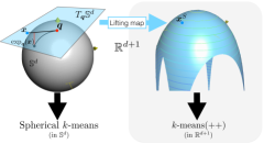
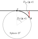
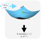
Figure 1: (L) Lifting map into $\mathbb{R}^{d}\times\mathbb{\mathbb{R}}$ for clustering on the sphere with k-means++. (M) $D_{\mathrm{rec}}$ in Eq. (15) in vertical thick red line. (R) Lifting map into $\mathbb{R}^{d}\times\mathbb{C}$ for the hyperboloid.

Our final application can be related to two problems that have received a steadily growing interest over the past decade in unsupervised machine learning: clustering on a non-linear manifold [Dhillon and Modha, 2001], and subspace custering [Vidal, 2011]. We consider two fundamental manifolds investigated by Galperin [1993] to compute centers of mass from relativistic theory: the sphere $\mathbb{S}^{d}$ and the hyperboloid $\mathbb{H}^{d}$, the former being of positive curvature, and the latter of negative curvature. Applications involving these specific manifolds are numerous in text processing, computer vision, geometric modelling, computer graphics, to name a few [Buss and Fillmore, 2001, Dhillon and Modha, 2001, Endo and Miyamoto, 2015, Kuang et al., 2014, Rong et al., 2010, Shahani et al., 2015, Straub et al., 2015a, b, c, 2014]. We emphasize the fact that the clustering problem has significant practical impact for $d$ as small as 2 in computer vision [Straub et al., 2014].

The problem is non-trivial for two separate reasons. First, the ambient space, i.e. the space of registration of the input data, is often implicitly Euclidean and therefore not the manifold [Dhillon and Modha, 2001]: if the mapping to the manifold is not carefully done, then geodesic distances measured on the manifold may be inconsistent with respect to the ambient space. Second, the fact that the manifold has non-zero curvature essentially prevents the direct use of Euclidean optimization algorithms [Zhang and Sra, 2016] — put simply, the average of two points that belong to a manifold does not necessarily belong to the manifold, so we have to be careful on how to compute centroids for hard clustering [Galperin, 1993, Nock et al., 2016, Rong et al., 2010, Schwander and Nielsen, 2013].

What we show now is that Riemannian manifolds with constant sectional curvature may be clustered with the $k$-means++ seeding for flat manifolds [Arthur and Vassilvitskii, 2007], without even touching a line of the algorithm. To formalise the problem, we need three key components of Riemannian geometry: tangent planes, exponential map and geodesics [Amari and Nagaoka, 2000]. We assume that the ambient space is a tangent plane to the manifold $\mathcal{M}$, which conveniently makes it look Euclidean (see Figure 1). The point of tangency is called $\bm{q}$, and the tangent plane $T_{\bm{q}}\mathcal{M}$. The exponential map, $\exp_{\bm{q}}:T_{\bm{q}}\mathcal{M}\rightarrow\mathcal{M}$, performs a distance preserving mapping: the geodesic length between $\bm{q}$ and $\exp_{\bm{q}}(\bm{x})$ in $\mathcal{M}$ is the same as the Euclidean length between $\bm{q}$ and $\bm{x}$ in $T_{\bm{q}}\mathcal{M}$. Our clustering objective is to find $\mathcal{C}\stackrel{{\scriptstyle\mathrm{.}}}{{=}}\{\bm{c}_{1},\bm{c}_{2},...\bm{c}_{k}\}\subset\mathcal{M}$ such that $D_{\mathrm{rec}}(\mathcal{S}:\mathcal{C})=\inf_{\mathcal{C}^{\prime}\subset\mathcal{M},|\mathcal{C}^{\prime}|=k}D_{\mathrm{rec}}(\mathcal{S},\mathcal{C}^{\prime})$, with

$$D_{\mathrm{rec}}(\mathcal{S},\mathcal{C}) \stackrel{{\scriptstyle\mathrm{.}}}{{=}}\sum_{i\in[m]_{*}}\min_{j\in[k]_{*}}D_{\mathrm{rec}}(\exp_{\bm{q}}(\bm{x}_{i}),\bm{c}_{j})\>\>,$$ (15)

where $D_{\mathrm{rec}}$ is a reconstruction loss, a function of the geodesic distance between $\exp_{\bm{q}}(\bm{x}_{i})$ and $\bm{c}_{j}$. We use two loss functions defined from Galperin [1993] and used in machine learning for more than a decade [Dhillon and Modha, 2001]:

$${\mathbb{R}}_{+}\ni D_{\mathrm{rec}}(\bm{y},\bm{c}) \stackrel{{\scriptstyle\mathrm{.}}}{{=}} \left\{\begin{array}[]{rcl}1-\cos D_{G}(\bm{y},\bm{c})&\mbox{for }&\mathcal{M}=\mathbb{S}^{d}\\ \cosh D_{G}(\bm{y},\bm{c})-1&\mbox{for }&\mathcal{M}=\mathbb{H}^{d}\end{array}\right.\>\>.$$ (18)

Here, $D_{G}(\bm{y},\bm{c})$ is the corresponding geodesic distance of $\mathcal{M}$ between $\bm{y}$ and $\bm{c}$. Figure 1 shows that $D_{\mathrm{rec}}(\bm{y},\bm{c})$ is the orthogonal distance between $T_{\bm{c}}\mathcal{M}$ and $\bm{y}$ when $\mathcal{M}=\mathbb{S}^{d}$. The solution to the clustering problem in eq. (15) is therefore the one that minimizes the error between tangent planes defined at the centroids, and points on the manifold.

(Sphere) S$k$-means++(${\mathcal{S}},k$)	(Hyperboloid) H$k$-means++(${\mathcal{S}},k$)
Input: dataset ${\mathcal{S}}\subset T_{\bm{q}}{\mathbb{S}^{d}},k\in{\mathbb{N}}_{*}$;   Step 1: ${\mathcal{S}}^{+}\leftarrow\{g^{-1}_{S}(\bm{x}^{S})\cdot\bm{x}^{S}:\bm{x}^{S}\in\mathrm{lift}({\mathcal{S}})\}$;   Step 2: ${\mathcal{C}}^{+}\leftarrow k\mbox{-means++$\_$seeding}({\mathcal{S}}^{+},k)$;   Step 3: ${\mathcal{C}}\leftarrow\exp^{-1}_{\bm{q}}({\mathcal{C}}^{+})$;   Output: Cluster centers ${\mathcal{C}}\in T_{\bm{q}}{\mathbb{S}^{d}}$;	Input: dataset ${\mathcal{S}}\subset T_{\bm{q}}{\mathbb{H}^{d}},k\in{\mathbb{N}}_{*}$;   Step 1: ${\mathcal{S}}^{+}\leftarrow\{g^{-1}_{H}(\bm{x}^{H})\cdot\bm{x}^{H}:\bm{x}^{H}\in\mathrm{lift}({\mathcal{S}})\}$;   Step 2: ${\mathcal{C}}^{+}\leftarrow k\mbox{-means++$\_$seeding}({\mathcal{S}}^{+},k)$;   Step 3: ${\mathcal{C}}\leftarrow\exp^{-1}_{\bm{q}}({\mathcal{C}}^{+})$;   Output: Cluster centers ${\mathcal{C}}\in T_{\bm{q}}{\mathbb{H}^{d}}$;
$\bm{x}^{S}\stackrel{{\scriptstyle\mathrm{.}}}{{=}}[x_{1}\quad x_{2}\quad\cdots\quad x_{d}\quad\|\bm{x}\|_{2}\cot\|\bm{x}\|_{2}]$	$\bm{x}^{H}\stackrel{{\scriptstyle\mathrm{.}}}{{=}}[x_{1}\quad x_{2}\quad\cdots\quad x_{d}\quad i\|\bm{x}\|_{2}\coth\|\bm{x}\|_{2}]$
$g_{S}(\bm{x}^{S})\stackrel{{\scriptstyle\mathrm{.}}}{{=}}\|\bm{x}\|_{2}/\sin\|\bm{x}\|_{2}$	$g_{H}(\bm{x}^{H})\stackrel{{\scriptstyle\mathrm{.}}}{{=}}-\|\bm{x}\|_{2}/\sinh\|\bm{x}\|_{2}$

Table 3: How to use $k$-means++ to cluster points on the sphere (left) or the hyperboloid (right).

It turns out that both distances in 18 can be engineered as Bregman divergences via Theorem 1, as seen in Table 2. Furthermore, they imply the same $\varphi$, which is just the generator of Mahalanobis distortion, but a different $g$. The construction involves a third party, a lifting map ($\mathrm{lift}(.)$) that increases the dimension by one. The Sphere lifting map $\mathbb{R}^{d}\ni\bm{x}\mapsto\bm{x}^{S}\in\mathbb{R}^{d+1}$ is indicated in Table 3 (left). The new coordinate depends on the norm of $\bm{x}$. The Hyperbolic lifting map, $\mathbb{R}^{d}\ni\bm{x}\mapsto\bm{x}^{H}\in\mathbb{R}^{d}\times\mathbb{C}$, involves a pure imaginary additional coordinate, is indicated in in Table 3 (right, with a slight abuse of notation) and Figure 1. Both $\bm{x}^{S}$ and $\bm{x}^{H}$ live on a $d$-dimensional manifold, depicted in Figure 1. When they are scaled by the corresponding $g_{.}(.)$, they happen to be mapped to $\mathbb{S}^{d}$ or $\mathbb{H}^{d}$, respectively, by what happens to be the manifold’s exponential map for the original $\bm{x}$ (see Appendix C).

Theorem 1 is interesting in this case because $\varphi$ corresponds to a Mahalanobis distortion: this shows that $k$-means++ seeding [Arthur and Vassilvitskii, 2007, Nock et al., 2008] can be used directly on the scaled coordinates ($g^{-1}_{\{S,H\}}(\bm{x}^{\{S,H\}})\cdot\bm{x}^{\{S,H\}}$) to pick centroids that yield an approximation of the global optimum for the clustering problem on the manifold which is just as good as the original Euclidean approximation bound [Arthur and Vassilvitskii, 2007].

Lemma 5

The expected potential of S$k$-means++ seeding over the random choices of $\mathcal{C}^{+}$ satisfies:

$$\mathbb{E}[D_{\mathrm{rec}}(\mathcal{S}:\mathcal{C})] \leq 8(2+\log k)\cdot\inf_{\mathcal{C}^{\prime}\in\mathbb{S}^{d}}D_{\mathrm{rec}}(\mathcal{S}:\mathcal{C}^{\prime})\>\>.$$ (19)

The same approximation bounds holds for H$k$-means++ seeding on the hyperboloid ($\mathcal{C}^{\prime},\mathcal{C}^{+}\in\mathbb{H}^{d}$).

Lemma 5 is notable since it was only recently shown that such a bound is possible for the sphere [Endo and Miyamoto, 2015], and to our knowledge, no such approximation quality is known for clustering on the hyperboloid [Rong et al., 2010, Schwander and Nielsen, 2013]. Notice that Lloyd iterations on non-linear manifolds would require repetitive renormalizations to keep centers on the manifold [Dhillon and Modha, 2001], an additional disadvantage compared to clustering on flat manifolds that $\{\mathrm{G,K}\}$-means++ seedings do not bear.

6 Experimental validation

We present some experiments validating our theoretical analysis for the applications above.

Multiple density ratio estimation. See Appendix H.1 for experiments in this domain.

Dual norm $p$-LMS (DN-$p$-LMS). We ran $p$-LMS and the DN-pLMS of §4 on the experimental setting of Kivinen et al. [2006]. We refer to that paper for an exhaustive description of the experimental setting, which we briefly summarize: it is a noisy signal processing setting, involving a dense or a sparse target. We compute, over the signal received, the error of our predictor on the signal. We keep all parameters as they are in [Kivinen et al., 2006], except for one: we make sure that data are scaled to fit in a $L_{p}$ ball of prescribed radius, to test the assumption related in [Kivinen et al., 2006] that fixing the learning rate $\eta_{t}$ is not straightforward in $p$-LMS. Knowing the true value of $X_{p}$, we then scale it by a misestimation factor $\rho$, typically in $[0.1,1.7]$. We use the same misestimation in DN-$p$-LMS. Thus, both algorithms suffer the same source of uncertainty. Also, we periodically change the signal (each 1000 iterations), to assess the performances of the algorithms in tracking changes in the signal.

$(p,q)=(1.17,6.9)$	$(p,q)=(2.0,2.0)$	$(p,q)=(6.9,1.17)$	$(p,q)=(1.17,6.9)$	$(p,q)=(2.0,2.0)$	$(p,q)=(6.9,1.17)$
$\rho=1.0$	$\rho=1.0$	$\rho=1.0$	$\rho=0.5$	$\rho=1.3$	$\rho=0.2$

Table 4: Summary of the experiments displaying ($y$) the error of $p$-LMS minus error of DN-$p$-LMS (when $>0$, DN-$p$-LMS beats $p$-LMS) as a function of $t$, in the setting of Kivinen et al. [2006], for various values of $(p,q)$ (columns). Left panel: (D)ense target; Right panel: (S)parse target.

Table 5: (L) Relative improvement (decrease) in $k$-means potential of SKM$\circ$S$k$-means++ compared to SKM alone. (R) Relative improvement of S$k$-means++ over Forgy initialization on the sphere.

Table 6: (L) % of the number of runs of SKM whose output (when it has converged) is better than S$k$-means++. (C) Maximal # of iterations for SKM after which it beats S$k$-means++ (ignoring runs of SKM that do not beat S$k$-means++). (R) Average # of iterations for SKM to converge.

Experiments, given in extenso in Appendix H.2, are sumarized in Table 4. The following trends emerge: in the mid to long run, DN-$p$-LMS is never beaten by $p$-LMS by more than a fraction of percent. On the other hand, DN-$p$-LM can beat $p$-LMS by very significant differences (exceeding 40$\%$), in particular when $p<2$, i.e. when we are outside the regime of the proof of Kivinen et al. [2006]. This indicates that significantly stronger and more general results than the one of Lemma 4 may be expected. Also, it seems that the problem of $p$-LMS lies in an “exploding” norm problem: in various cases, we observe that $\|\bm{w}_{t}\|$ (in any norm) blows up with $t$, and this correlates with a very significant degradation of its performances. Clearly, DN-$p$-LMS does not have this problem since all relevant norms are under tight control. Finally, even when the norm does not explode, DN-$p$-LMS can still beat $p$-LMS, by less important differences though. Of course, the output of $p$-LMS can repeatedly be normalised, but the normalisation would escape the theory of Kivinen et al. [2006] and it is not clear which kind of normalisation would bring the best results.

Clustering on the sphere. For $k\in[50]_{*}$, we simulate on $T_{\bm{0}}{\mathbb{S}}^{2}$ a mixture of spherical Gaussian and uniform densities with $2k$ components. We run three algorithms: (i) SKM [Dhillon and Modha, 2001] on the data embedded on ${\mathbb{S}}^{2}$ with random (Forgy) initialization, (ii), S$k$-means++ and (iii) SKM with S$k$-means++ initialisation. Results are averaged over the algorithms’ runs.

Table 5 (left) displays that using S$k$-means++ as initialization for SKM brings a very significant leverage over SKM alone, since we almost divide the $k$-means potential by a factor 2 on some runs. The right plot of Table 5 shows that s-$k$-means++ consistently reduces the $k$-means potential by at least a factor 2 over Forgy. The left plot in Table 6 displays that even when it has converged, SKM does not necessarily beat S$k$-means++. Finally, the center+right plots in Table 6 display that even when it does beat S$k$-means++ when it has converged, the iteration number after which SKM beats S$k$-means++ increases with $k$, and in the worst case may exceed the average number of iterations needed for SKM to converge (we stopped SKM if relative improvement is not above $1{}^{\text{o}}\mkern-5.0mu/\mkern-3.0mu_{\text{oo}}$).

7 Conclusion

We presented a new scaled Bregman identity (Theorem 1), and used it to derive novel results in multiple density ratio estimation, adaptive filtering, and clustering on curved manifolds. We believe that, like other established properties of Bregman divergences, there is potential for several other applications of the result; Appendix E, F present preliminary thoughts in this direction.

Appendix A Additional helper lemmas

We begin with some helper lemmas that will be used in some of the proofs. In what follows, let

$$\varphi_{q}(\bm{w}) =(1/2)(W^{2}+\|\bm{w}\|_{q}^{2})$$

$$\varphi^{\dagger}_{q}(\bm{w}) =W\cdot\|\bm{w}\|_{q}$$

for some $W>0$ and $p,q\in(1,\infty)$ such that $1/p+1/q=1$.

A.1 Properties of $\varphi_{q}$ and $\varphi_{q}^{\dagger}$

We use the following properties of $\varphi,\varphi^{\dagger}$.

Lemma 6

For any $\bm{w}$,

$$\nabla\varphi_{q}(\bm{w}) =\|\bm{w}\|_{q}^{2-q}\cdot\mathrm{sign}(\bm{w})\otimes|\bm{w}|^{q-1}$$

$$\nabla\varphi_{q}^{\dagger}(\bm{w}) =W\cdot\|\bm{w}\|_{q}^{1-q}\cdot\mathrm{sign}(\bm{w})\otimes|\bm{w}|^{q-1},$$

where $\otimes$ denotes Hadamard product.

Proof.

The first identity was shown in Kivinen et al. [2006, Example 1]. The second identity follows from a simple calculation. ∎

This implies the follows useful relation between the gradients of $\varphi_{q}$ and $\varphi_{q}^{\dagger}$.

Corollary 7

For any $\bm{w}$,

$$\nabla\varphi_{q}(\bm{w}) =(\|\bm{w}\|_{q}/W)\cdot\nabla\varphi^{\dagger}_{q}(\bm{w})$$

$$\|\nabla\varphi^{\dagger}_{q}(\bm{w})\|_{p} =W$$

$$\|\nabla\varphi_{q}(\bm{w})\|_{p} =\|\bm{w}\|_{q}.$$

Proof of Corollary 7.

The proof follows by direct application of Lemma 6 and the definition of $p,q$. Note the third identity was shown in Kivinen et al. [2006, Appendix I]. ∎

As a consequence, we conclude that the gradients of $\varphi$ and $\varphi^{\dagger}$ coincide when considering vectors on the $W$-sphere.

Lemma 8

For any $\|\bm{w}\|_{q}=W$,

$$\nabla\varphi_{q}\left(\bm{w}\right)=\nabla\varphi_{q}^{\dagger}\left(\bm{w}\right).$$

Proof.

This follows from the relation between $\nabla\varphi_{q}$ and $\nabla\varphi_{q}^{\dagger}$ from Lemma 6. ∎

Finally, we have the following result about the composition of gradients.

Lemma 9

For any $\bm{w}$,

$$\nabla\varphi_{q}\circ{\nabla\varphi_{p}^{\dagger}}(\bm{w}) =\nabla\varphi^{\dagger}_{q}\circ{\nabla\varphi_{p}^{\dagger}}(\bm{w})=\frac{W}{\|\bm{w}\|_{p}}\cdot\bm{w}.$$

Proof.

For the first identity, applying Lemma 6 twice,

$$\nabla\varphi_{q}\circ{\nabla\varphi_{p}^{\dagger}}(\bm{w}) = \frac{1}{\|{\nabla\varphi_{p}^{\dagger}}(\bm{w})\|_{q}^{q-2}}\cdot\mathrm{sign}({\nabla\varphi_{p}^{\dagger}}(\bm{w}))\otimes|{\nabla\varphi_{p}^{\dagger}}(\bm{w})|^{q-1}$$ (20)

$$= \frac{1}{W^{q-2}_{q}}\cdot\mathrm{sign}(\bm{w})\otimes\frac{W^{q-1}}{\|\bm{w}\|_{p}^{(p-1)(q-1)}}\cdot|\bm{w}|^{(p-1)(q-1)}$$

$$= \frac{W}{\|\bm{w}\|_{p}}\cdot\bm{w}\>\>.$$

For the second identity, use Corollary 7 to conclude that

$$\nabla\varphi^{\dagger}_{q}\circ{\nabla\varphi_{p}^{\dagger}}(\bm{w}) =\frac{W}{\|\nabla\varphi_{p}^{\dagger}(\bm{w})\|_{q}}\cdot\nabla\varphi_{q}(\nabla\varphi_{p}^{\dagger}(\bm{w}))$$

$$=W\cdot\frac{\bm{w}}{\|\bm{w}\|_{p}}.$$

∎

A.2 Bound on successive iterate divergence

The following Lemma extends [Kivinen et al., 2006, Appendix I] to $\varphi^{\dagger}$.

Lemma 10

For any $\bm{w}$ and $\bm{\delta}$,

$$D_{\varphi^{\dagger}_{q}}\left(\bm{w}\|{\nabla\varphi_{p}^{\dagger}}\left(\nabla\varphi_{q}^{\dagger}(\bm{w})+\bm{\delta}\right)\right)$$ (21)

$$\leq \frac{(p-1)\|\bm{w}\|_{q}W}{2}\cdot\left\|\frac{1}{\|\nabla\varphi_{q}^{\dagger}(\bm{w})+\bm{\delta}\|_{p}}\cdot\left(\nabla\varphi_{q}^{\dagger}(\bm{w})+\bm{\delta}\right)-\frac{1}{W}\cdot\nabla\varphi^{\dagger}_{q}\left(\bm{w}\right)\right\|_{p}^{2}\>\>.$$

Proof of Lemma 10.

In this proof, $\circ$ denotes composition and $\otimes$ is Hadamard product. The key step in the proof is the use of Theorem 1 to “branch” on the proof of [Kivinen et al., 2006, Appendix I] on the first following identity (letting $\varphi_{q}(\bm{w})\stackrel{{\scriptstyle\mathrm{.}}}{{=}}(1/2)\cdot(W^{2}+\|\bm{w}\|_{q}^{2})$). We also make use of the dual symmetry of Bregman divergences and we obtain third identity of:

$$D_{\varphi^{\dagger}_{q}}\left(\bm{w}\|{\nabla\varphi_{p}^{\dagger}}\left(\nabla\varphi_{q}^{\dagger}(\bm{w})+\bm{\delta}\right)\right)$$

$$= \frac{\|\bm{w}\|_{q}}{W}\cdot D_{\varphi_{q}}\left(\frac{W}{\|\bm{w}\|_{q}}\cdot\bm{w}\left\|\frac{W}{\|\nabla\varphi_{p}^{\dagger}(\nabla\varphi_{q}^{\dagger}(\bm{w})+\bm{\delta})\|_{q}}\cdot{\nabla\varphi_{p}^{\dagger}}\left(\nabla\varphi_{q}^{\dagger}(\bm{w})+\bm{\delta}\right.\right)\right)$$

$$= \frac{\|\bm{w}\|_{q}}{W}\cdot D_{\varphi_{q}}\left(\frac{W}{\|\bm{w}\|_{q}}\cdot\bm{w}\left\|{\nabla\varphi_{p}^{\dagger}}\left(\nabla\varphi_{q}^{\dagger}(\bm{w})+\bm{\delta}\right.\right)\right)$$

$$= \frac{\|\bm{w}\|_{q}}{W}\cdot D_{\varphi_{p}}\left(\nabla\varphi_{q}\circ{\nabla\varphi_{p}^{\dagger}}\left(\nabla\varphi_{q}^{\dagger}(\bm{w})+\bm{\delta}\right)\left\|\nabla\varphi_{q}\left(\frac{W}{\|\bm{w}\|_{q}}\cdot\bm{w}\right)\right.\right)\text{ by dual symmetry }$$

$$= \frac{\|\bm{w}\|_{q}}{W}\cdot D_{\varphi_{p}}\left(\frac{W}{\|\nabla\varphi_{q}^{\dagger}(\bm{w})+\bm{\delta}\|_{p}}\cdot\left(\nabla\varphi_{q}^{\dagger}(\bm{w})+\bm{\delta}\right)\left\|\frac{W}{\|\bm{w}\|_{q}}\cdot\nabla\varphi_{q}\left(\bm{w}\right)\right.\right)$$ (23)

$$= \frac{\|\bm{w}\|_{q}}{W}\cdot D_{\varphi_{p}}\left(\frac{W}{\|\nabla\varphi_{q}^{\dagger}(\bm{w})+\bm{\delta}\|_{p}}\cdot\left(\nabla\varphi_{q}^{\dagger}(\bm{w})+\bm{\delta}\right)\left\|\nabla\varphi^{\dagger}_{q}\left(\bm{w}\right)\right.\right)$$ (24)

$$= \|\bm{w}\|_{q}W\cdot D_{\varphi_{p}}\left(\frac{1}{\|\nabla\varphi_{q}^{\dagger}(\bm{w})+\bm{\delta}\|_{p}}\cdot\left(\nabla\varphi_{q}^{\dagger}(\bm{w})+\bm{\delta}\right)\left\|\frac{1}{W}\cdot\nabla\varphi^{\dagger}_{q}\left(\bm{w}\right)\right.\right)\>\>.$$ (25)

Equations (A.2) – (24) hold because of Corollary 7. We now use Appendix I in Kivinen et al. [2006] on Equation (25) and obtain

$$D_{\varphi^{\dagger}_{q}}\left(\bm{w}\|{\nabla\varphi_{p}^{\dagger}}\left(\nabla\varphi_{q}^{\dagger}(\bm{w})+\bm{\delta}\right)\right)$$

$$\leq \frac{(p-1)\|\bm{w}\|_{q}W}{2}\cdot\left\|\frac{1}{\|\nabla\varphi_{q}^{\dagger}(\bm{w})+\bm{\delta}\|_{p}}\cdot\left(\nabla\varphi_{q}^{\dagger}(\bm{w})+\bm{\delta}\right)-\frac{1}{W}\cdot\nabla\varphi^{\dagger}_{q}\left(\bm{w}\right)\right\|_{p}^{2}\>\>,$$

as claimed. ∎

A.3 Bound on successive iterate divergence to target

In what follows, we write the DN-pLMS updates as $\bm{w}_{t}=\nabla\varphi_{p}^{\dagger}(\bm{\theta}_{t})$, where

$$\bm{\theta}_{t}\stackrel{{\scriptstyle\mathrm{.}}}{{=}}\nabla\varphi_{q}^{\dagger}(\bm{w}_{t-1})-\Delta_{t}$$

for $\Delta_{t}=\eta_{t}\cdot(\bm{w}_{t-1}^{\top}\bm{x}_{t}-y_{t})\cdot\bm{x}_{t}$. Further, for notational ease, we write

$$\bar{\bm{u}}\stackrel{{\scriptstyle\mathrm{.}}}{{=}}\frac{\bm{u}}{g_{q}(\bm{u})}$$

and

$$\bar{\bm{\theta}}_{t}\stackrel{{\scriptstyle\mathrm{.}}}{{=}}\frac{\bm{\theta}_{t}}{\|\bm{\theta}_{t}\|_{p}}.$$

We have the following preliminary bound on the distance from iterates of DN-pLMS to the (normalised) target.

Lemma 11

Fix any learning rate sequence $\{\eta_{t}\}_{t=1}^{T}$. Pick any $\bm{u}$, and consider iterates $\{\bm{w}_{t}\}_{t=0}^{T}$ as per Equation 10. Denote $s_{t}\stackrel{{\scriptstyle\mathrm{.}}}{{=}}(\bar{\bm{u}}-\bm{w}_{t-1})^{\top}\bm{x}_{t},r_{t}\stackrel{{\scriptstyle\mathrm{.}}}{{=}}\bar{\bm{u}}^{\top}\bm{x}_{t}-y_{t}$, and $\upalpha_{t}\stackrel{{\scriptstyle\mathrm{.}}}{{=}}\frac{W}{\|\bm{\theta}_{t}\|_{p}}$. Suppose $\|\bm{x}_{t}\|_{p}\leq X_{p}$. Then,

$$D_{\varphi_{q}}\left(\bar{\bm{u}}\left\|\bm{w}_{t-1}\right.\right)-D_{\varphi_{q}}\left(\bar{\bm{u}}\left\|\bm{w}_{t}\right.\right) \geq Q+R+S+T\>\>,$$

with

$$Q \stackrel{{\scriptstyle\mathrm{.}}}{{=}} \frac{\upalpha_{t}}{2}\eta_{t}(s^{2}_{t}-r^{2}_{t}),$$

$$R \stackrel{{\scriptstyle\mathrm{.}}}{{=}} (1-\upalpha_{t})\cdot\underbrace{\left(W^{2}-\bar{\bm{u}}^{\top}\nabla\varphi_{q}^{\dagger}(\bm{w}_{t-1})\right)}_{\in[0,2W^{2}]}\>\>,$$

$$S \stackrel{{\scriptstyle\mathrm{.}}}{{=}} \frac{p-1}{2}\cdot\underbrace{\left(2\upalpha^{2}_{t}\eta^{2}_{t}(s_{t}-r_{t})^{2}X_{p}^{2}-\left\|(s_{t}-r_{t})\eta_{t}\upalpha_{t}\cdot\bm{x}_{t}-(1-\upalpha_{t})\cdot\nabla\varphi_{q}^{\dagger}(\bm{w}_{t-1})\right\|_{p}^{2}\right)}_{\geq-2(1-\upalpha_{t})^{2}W^{2}}\>\>,$$

$$T \stackrel{{\scriptstyle\mathrm{.}}}{{=}} \frac{\upalpha_{t}}{2}\eta_{t}(s_{t}-r_{t})^{2}\left(1-2(p-1)\eta_{t}\upalpha_{t}X_{p}^{2}\right)\>\>.$$

Proof of Lemma 11.

The Bregman triangle equality (also called the three points property) [Boissonnat et al., 2010, Property 5], [Cesa-Bianchi and Lugosi, 2006, Lemma 11.1] brings:

$$D_{\varphi_{q}}\left(\bar{\bm{u}}\left\|\bm{w}_{t-1}\right.\right)-D_{\varphi_{q}}\left(\bar{\bm{u}}\left\|\bm{w}_{t}\right.\right)$$

$$= \left(\bar{\bm{u}}-\bm{w}_{t-1}\right)^{\top}\left(\nabla\varphi_{q}\left(\bm{w}_{t}\right)-\nabla\varphi_{q}\left(\bm{w}_{t-1}\right)\right)-D_{\varphi_{q}}\left(\bm{w}_{t-1}\left\|\bm{w}_{t}\right.\right)$$

$$= \left(\bar{\bm{u}}-\bm{w}_{t-1}\right)^{\top}\left(\nabla\varphi_{q}^{\dagger}\left(\bm{w}_{t}\right)-\nabla\varphi_{q}^{\dagger}\left(\bm{w}_{t-1}\right)\right)-D_{\varphi_{q}^{\dagger}}\left(\bm{w}_{t-1}\left\|\bm{w}_{t}\right.\right)\text{ by Lemmas \ref{lemm:plms-update-norm}, \ref{lemm:gradient-same} }\>\>.$$

We now have

$$\nabla\varphi_{q}^{\dagger}\left(\bm{w}_{t}\right)=\nabla\varphi_{q}^{\dagger}\circ{\nabla\varphi_{p}^{\dagger}}(\bm{\theta}_{t})=W\cdot\bar{\bm{\theta}}_{t}\>\>$$

by Corollary 7. We get

$$D_{\varphi_{q}}\left(\bar{\bm{u}}\left\|\bm{w}_{t-1}\right.\right)-D_{\varphi_{q}}\left(\bar{\bm{u}}\left\|\bm{w}_{t}\right.\right)$$

$$\geq \left(\bar{\bm{u}}-\bm{w}_{t-1}\right)^{\top}\left(W\cdot\bar{\bm{\theta}}_{t}-\nabla\varphi_{q}^{\dagger}(\bm{w}_{t-1})\right)-\frac{(p-1)W^{2}}{2}\cdot\left\|\bar{\bm{\theta}}_{t}-\frac{1}{W}\cdot\nabla\varphi^{\dagger}_{q}\left(\bm{w}_{t-1}\right)\right\|_{p}^{2}$$

$$= \left(\bar{\bm{u}}-\bm{w}_{t-1}\right)^{\top}\left(W\cdot\bar{\bm{\theta}}_{t}-\nabla\varphi_{q}^{\dagger}(\bm{w}_{t-1})\right)-\frac{p-1}{2}\cdot\left\|W\cdot\bar{\bm{\theta}}_{t}-\nabla\varphi^{\dagger}_{q}\left(\bm{w}_{t-1}\right)\right\|_{p}^{2}.$$

Now, note that

$$\bm{\theta}_{t}=\nabla\varphi_{q}^{\dagger}(\bm{w}_{t-1})+\eta_{t}\cdot(s_{t}-r_{t})\cdot\bm{x}_{t}.$$

We can thus rewrite the above as

$$D_{\varphi_{q}}\left(\bar{\bm{u}}\left\|\bm{w}_{t-1}\right.\right)-D_{\varphi_{q}}\left(\bar{\bm{u}}\left\|\bm{w}_{t}\right.\right)$$

$$\geq s_{t}(s_{t}-r_{t})\eta_{t}\upalpha_{t}+(1-\upalpha_{t})\left(\bm{w}_{t-1}^{\top}\nabla\varphi_{q}^{\dagger}(\bm{w}_{t-1})-\bar{\bm{u}}^{\top}\nabla\varphi_{q}^{\dagger}(\bm{w}_{t-1})\right)$$

$$-\frac{p-1}{2}\cdot\left\|(s_{t}-r_{t})\eta_{t}\upalpha_{t}\cdot\bm{x}_{t}-(1-\upalpha_{t})\cdot\nabla\varphi_{q}^{\dagger}(\bm{w}_{t-1})\right\|_{p}^{2}$$

$$= s_{t}(s_{t}-r_{t})\eta_{t}\upalpha_{t}+(1-\upalpha_{t})\left(W^{2}-\bar{\bm{u}}^{\top}\nabla\varphi_{q}^{\dagger}(\bm{w}_{t-1})\right)$$

$$-\frac{p-1}{2}\cdot\left\|(s_{t}-r_{t})\eta_{t}\upalpha_{t}\cdot\bm{x}_{t}-(1-\upalpha_{t})\cdot\nabla\varphi_{q}^{\dagger}(\bm{w}_{t-1})\right\|_{p}^{2}\text{ by definition of }\nabla\varphi_{q}^{\dagger}$$

$$= Q+R+S+T\>\>.$$

∎

We can show that the sum $R+S+T\geq 0$. This proof involves chaining together multiple simple inequalities. We give a high level overview in Figure 2.

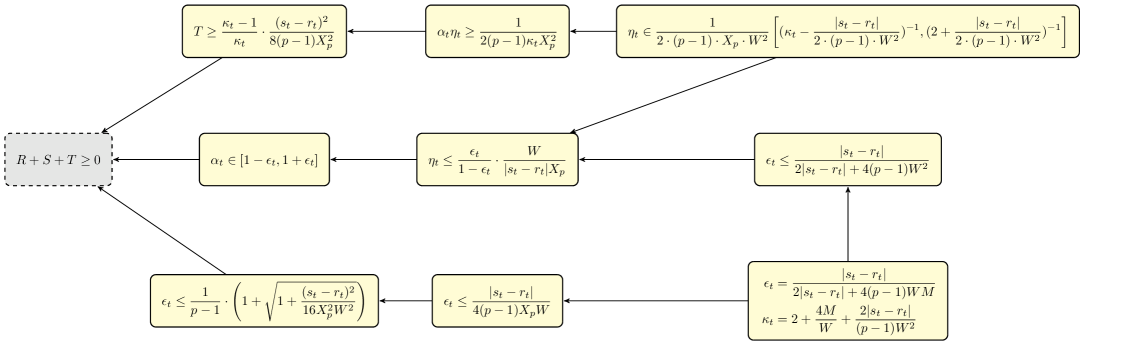
Figure 2: Schematic of proof of Lemma 12. Arrows from equation $A$ to $B$ indicate that $A\implies B$.

Lemma 12

Let $R,S,T$ be as per Lemma 11. Suppose we fix

$$\eta_{t} = \upgamma\cdot\frac{W}{4(p-1)MX_{p}W+|y_{t}-\bm{w}_{t-1}^{\top}\bm{x}_{t}|X_{p}}\>\>,$$ (26)

for any $\upgamma\in[1/2,1]$, and $M\stackrel{{\scriptstyle\mathrm{.}}}{{=}}\max\{W,X_{p}\}$. Then, $T+R+S\geq 0$.

Proof.

The triangle inequality and the fact that $\|\nabla\varphi_{q}^{\dagger}(\bm{w}_{t-1})\|_{p}=W$ brings

$$\upalpha_{t} \in \left[\frac{W}{\|\nabla\varphi_{q}^{\dagger}(\bm{w}_{t-1})\|_{p}+\eta_{t}|s_{t}-r_{t}|\cdot\|\bm{x}_{t}\|_{p}},\frac{W}{\|\nabla\varphi_{q}^{\dagger}(\bm{w}_{t-1})\|_{p}-\eta_{t}|s_{t}-r_{t}|\cdot\|\bm{x}_{t}\|_{p}}\right]$$ (27)

$$\subseteq\left[\frac{W}{W+\eta_{t}|s_{t}-r_{t}|X_{p}},\frac{W}{W-\eta_{t}|s_{t}-r_{t}|\cdot X_{p}}\right],$$

assuming that $\eta_{t}$ is chosen so that

$$\eta_{t} \leq \frac{W}{|s_{t}-r_{t}|\cdot X_{p}}\>\>,$$ (28)

so that the right bound is non negative. To indeed ensure this, suppose that for some $0<\epsilon_{t}\leq 1/2$, we fix

$$\eta_{t} \leq \frac{\epsilon_{t}}{1-\epsilon_{t}}\cdot\frac{W}{|s_{t}-r_{t}|X_{p}}\>\>.$$ (29)

We would in addition obtain from Equation (27) that $\upalpha_{t}\in[1-\epsilon_{t},1+\epsilon_{t}]$. Suppose $\eta_{t}$ is also fixed to ensure

$$\eta_{t} \in \left[\frac{W}{2(p-1)\upkappa_{t}X_{p}W^{2}-|s_{t}-r_{t}|X_{p}},\frac{W}{4(p-1)X_{p}W^{2}+|s_{t}-r_{t}|X_{p}}\right]\>\>,$$ (30)

for some $\upkappa_{t}$ such that

$$\upkappa_{t} \geq 2+\frac{|s_{t}-r_{t}|}{(p-1)W^{2}}\>\>.$$ (31)

Notice that constraint on $\upkappa_{t}$ makes the interval non empty and its left bound strictly positive. Assuming (30) holds, we would have

$$\upalpha_{t}\eta_{t} \in \left[\frac{1}{2(p-1)\upkappa_{t}X_{p}^{2}},\frac{1}{4(p-1)X_{p}^{2}}\right]\>\>.$$ (32)

The left bound of (32) holds because

$$\upalpha_{t}\eta_{t} \geq \eta_{t}\cdot\frac{W}{W+\eta_{t}|s_{t}-r_{t}|X_{p}}$$ (33)

$$\geq \frac{1}{2(p-1)\upkappa_{t}X_{p}^{2}}\>\>.$$

The first inequality holds because of (27) and the second one holds because of (30). The right bound of (32) holds because of (27), and so

$$\upalpha_{t}\eta_{t} \leq \eta_{t}\cdot\frac{W}{W-\eta_{t}|s_{t}-r_{t}|X_{p}}$$ (34)

$$\leq \frac{1}{4(p-1)X_{p}^{2}}\>\>,$$

where the last inequality is due to (30).

Equation (32) makes that $T(\eta_{t}\upalpha_{t})$ is at least its value when $\upalpha_{t}\eta_{t}$ attains the lower bound of (33), that is,

$$T(\eta_{t}\upalpha_{t}) \geq \frac{\upkappa_{t}-1}{\upkappa_{t}}\cdot\frac{(s_{t}-r_{t})^{2}}{8(p-1)X_{p}^{2}}\>\>.$$ (35)

Now, to guarantee $\upalpha_{t}\in[1-\epsilon_{t},1+\epsilon_{t}]$, it is sufficient that the right-hand side of inequality (29) belongs to interval (30) and we pick $\eta_{t}$ within the interval [left bound (30), right-hand side (29)]. To guarantee that the right-hand side of inequality (29) falls in interval (30), we need first,

$$\frac{W}{2(p-1)\upkappa_{t}X_{p}W^{2}-|s_{t}-r_{t}|X_{p}} \leq \frac{\epsilon_{t}}{1-\epsilon_{t}}\cdot\frac{W}{|s_{t}-r_{t}|X_{p}}\>\>,$$ (36)

that is,

$$\upkappa_{t} \geq \frac{1}{\epsilon_{t}}\cdot\frac{|s_{t}-r_{t}|}{2(p-1)W^{2}}\>\>.$$ (37)

To guarantee that the right-hand side of inequality (29) falls in interval (30) we need then

$$\frac{W}{4(p-1)X_{p}W^{2}+|s_{t}-r_{t}|X_{p}} \geq \frac{\epsilon_{t}}{1-\epsilon_{t}}\cdot\frac{W}{|s_{t}-r_{t}|X_{p}}\>\>,$$ (38)

that is,

$$\epsilon_{t} \leq \frac{|s_{t}-r_{t}|}{2|s_{t}-r_{t}|+4(p-1)W^{2}}\>\>.$$ (39)

To summarize, if we pick any strictly positive $\epsilon_{t}$ following inequality (39) (note $\epsilon_{t}<1$) and

$$\upkappa_{t} \stackrel{{\scriptstyle\mathrm{.}}}{{=}} 2+\frac{1}{\epsilon_{t}}\cdot\frac{|s_{t}-r_{t}|}{(p-1)W^{2}}\>\>,$$ (40)

then we shall have both $\upalpha_{t}\in[1-\epsilon_{t},1+\epsilon_{t}]$ and inequality (35) holds as well. In this case, we shall have

$$T+R+S \geq \left(1-\frac{1}{2+\frac{1}{\epsilon_{t}}\cdot\frac{|s_{t}-r_{t}|}{(p-1)W^{2}}}\right)\cdot\frac{(s_{t}-r_{t})^{2}}{8(p-1)X_{p}^{2}}-2\epsilon_{t}W^{2}-(p-1)\epsilon_{t}^{2}W^{2}$$ (41)

$$\geq \left(1-\frac{1}{2}\right)\cdot\frac{(s_{t}-r_{t})^{2}}{8(p-1)X_{p}^{2}}-2\epsilon_{t}W^{2}-(p-1)\epsilon_{t}^{2}W^{2}$$

$$=\frac{(s_{t}-r_{t})^{2}}{16(p-1)X_{p}^{2}}-2\epsilon_{t}W^{2}-(p-1)\epsilon_{t}^{2}W^{2}\>\>.$$

To finish up, we want to solve for $\epsilon_{t}$ the right-hand side such that it is non negative, and we find that $\epsilon_{t}$ has to satisfy

$$\epsilon_{t} \leq \frac{1}{p-1}\cdot\left(1+\sqrt{1+\frac{(s_{t}-r_{t})^{2}}{16X_{p}^{2}W^{2}}}\right)\>\>.$$ (42)

Since $\sqrt{1+x}\geq\sqrt{x}$, a sufficient condition is

$$\epsilon_{t} \leq \frac{|s_{t}-r_{t}|}{4(p-1)X_{p}W}\>\>.$$ (43)

To ensure this and inequality (39), it is sufficient that we fix

$$\epsilon_{t} \stackrel{{\scriptstyle\mathrm{.}}}{{=}} \frac{|s_{t}-r_{t}|}{2|s_{t}-r_{t}|+4(p-1)WM}\>\>,$$ (44)

where $M\stackrel{{\scriptstyle\mathrm{.}}}{{=}}\max\{W,X_{p}\}$. With this expression for $\epsilon_{t}$, we get from (40),

$$\upkappa_{t} \stackrel{{\scriptstyle\mathrm{.}}}{{=}} 2+\frac{4M}{W}+\frac{2|s_{t}-r_{t}|}{(p-1)W^{2}}\>\>.$$ (45)

For these choices, Lemma 13 implies that the given $\eta_{t}$ is feasible. ∎

Lemma 13

Suppose $\epsilon_{t}$ satisfies (44) and $\upkappa_{t}$ satisfies (45). Then, a sufficient condition for $\eta_{t}$ to satisfy both (29) and (30) is

$$\eta_{t} = \upgamma\cdot\frac{W}{4(p-1)MX_{p}W+|y_{t}-\bm{w}_{t-1}^{\top}\bm{x}_{t}|X_{p}}\>\>,$$

for any $\upgamma\in[1/2,1]$.

Proof of Lemma 13.

Notice the range of values authorized for $\eta_{t}$:

$$\eta_{t} \in \left[\frac{W}{2(p-1)\upkappa_{t}X_{p}W^{2}-|s_{t}-r_{t}|X_{p}},\frac{\epsilon_{t}}{1-\epsilon_{t}}\cdot\frac{W}{|s_{t}-r_{t}|X_{p}}\right]$$ (46)

$$=\left[\frac{W}{2(p-1)\left(2+\frac{4M}{W}+\frac{2|s_{t}-r_{t}|}{(p-1)W^{2}}\right)X_{p}W^{2}-|s_{t}-r_{t}|X_{p}},\frac{W}{4(p-1)MX_{p}W+|s_{t}-r_{t}|X_{p}}\right]$$

$$=\left[\frac{W}{2(2(p-1)W^{2}+4M(p-1)W+2|s_{t}-r_{t}|)X_{p}-|s_{t}-r_{t}|X_{p}},\frac{W}{4(p-1)MX_{p}W+|s_{t}-r_{t}|X_{p}}\right]$$

$$=\left[\frac{W}{4(p-1)X_{p}W^{2}+8(p-1)MX_{p}W+3|s_{t}-r_{t}|X_{p}},\frac{W}{4(p-1)MX_{p}W+|s_{t}-r_{t}|X_{p}}\right]$$

$$\supset \left[\frac{W}{8(p-1)MX_{p}W+2|s_{t}-r_{t}|X_{p}},\frac{W}{4(p-1)MX_{p}W+|s_{t}-r_{t}|X_{p}}\right]\>\>.$$

A sufficient condition for $\eta_{t}$ to fall in interval (46) is

$$\eta_{t} = \upgamma\cdot\frac{W}{4(p-1)MX_{p}W+|y_{t}-\bm{w}_{t-1}^{\top}\bm{x}_{t}|X_{p}}\>\>,$$

for any $\upgamma\in[1/2,1]$. ∎

Lemma 14

Suppose we fix the learning rate as per (26). Pick any $\bm{u}$, and consider iterates $\{\bm{w}_{t}\}_{t=0}^{T}$ as per Equation 10. Suppose $\|\bm{x}_{t}\|_{p}\leq X_{p}$ and $|y_{t}|\leq Y,\forall t\leq T$. Then, for any $t$,

$$D_{\varphi_{q}}\left(\bar{\bm{u}}\left\|\bm{w}_{t-1}\right.\right)-D_{\varphi_{q}}\left(\bar{\bm{u}}\left\|\bm{w}_{t}\right.\right)\geq\frac{1}{4(p-1)\left(2+\frac{4M}{W}+\frac{2(Y+X_{p}W)}{(p-1)W^{2}}\right)X_{p}^{2}}\cdot(s^{2}_{t}-r^{2}_{t})$$

where $s_{t}\stackrel{{\scriptstyle\mathrm{.}}}{{=}}(\bar{\bm{u}}-\bm{w}_{t-1})^{\top}\bm{x}_{t}$, $r_{t}\stackrel{{\scriptstyle\mathrm{.}}}{{=}}\bar{\bm{u}}^{\top}\bm{x}_{t}-y_{t}$.

Proof of Lemma 14.

We start from the bound of Lemma 11:

$$D_{\varphi_{q}}\left(\bar{\bm{u}}\left\|\bm{w}_{t-1}\right.\right)-D_{\varphi_{q}}\left(\bar{\bm{u}}\left\|\bm{w}_{t}\right.\right) \geq Q+R+S+T$$ (47)

$$\geq Q\text{ by Lemma \ref{lemm:rst} }$$

$$= \frac{\upalpha_{t}}{2}\eta_{t}(s^{2}_{t}-r^{2}_{t})\text{ by definition }$$

$$\geq \frac{1}{4(p-1)\upkappa_{t}X_{p}^{2}}\cdot(s^{2}_{t}-r^{2}_{t})$$

$$\geq \frac{1}{4(p-1)\left(2+\frac{4M}{W}+\frac{2\max_{t}|y_{t}-\bm{w}_{t-1}^{\top}\bm{x}_{t}|}{(p-1)W^{2}}\right)X_{p}^{2}}\cdot(s^{2}_{t}-r^{2}_{t})$$

$$\geq \frac{1}{4(p-1)\left(2+\frac{4M}{W}+\frac{2(Y+X_{p}W)}{(p-1)W^{2}}\right)X_{p}^{2}}\cdot(s^{2}_{t}-r^{2}_{t})\>\>.$$

The last constraint to check for this bound to be valid is our $\epsilon_{t}$ in (44) has to be $<1/2$ from inequality (28), which trivially holds since $4(p-1)WM\geq 0$.

We conclude by noting Lemma 13 provides a feasible value of $\eta_{t}$. ∎

A.4 Gauge normalisation

The following lemma about the gauge of $\bm{x}$ will be useful.

Lemma 15

Let $g_{q}(\bm{x})=\|\bm{x}\|_{q}/W$ for some $W>0$. Then, for the iterates $\{\bm{w}_{t}\}$ as per Equation 9, $g_{q}(\bm{w}_{t})=1$.

Proof.

We have

$$g_{q}(\bm{w}_{t}) = \frac{\|\bm{w}_{t}\|_{q}}{W}$$ (48)

$$= \frac{W}{W}\text{ by Lemma \ref{lemm:plms-update-norm} }$$

$$= 1\>\>,\forall t\geq 1\>\>.$$

∎

Appendix B Proofs of results in main body

We present proofs of all results in the main body.

Proof of Theorem 1.

Let $\mbox{{\small{J}}}:\mathcal{X}\rightarrow\mathcal{X}_{g}$ denote the Jacobian of $h\colon\bm{x}\mapsto(1/g(\bm{x}))\cdot\bm{x}$. By an elementary calculation,

$$g(\bm{x})\cdot\mbox{{\small{J}}}=\mbox{{\small{I}}}_{d}-(1/g(\bm{x}))\cdot\bm{x}\nabla g(\bm{x})^{\top},$$

which by the chain rule brings the following expression for the gradient of $\varphi^{\dagger}(\bm{y})=g(\bm{y})\cdot(\varphi\circ h)(\bm{y})$:

$$\nabla\varphi^{\dagger}\left(\bm{y}\right) =\nabla g(\bm{y})\cdot(\varphi\circ h)(\bm{y})+g(\bm{y})\cdot\nabla(\varphi\circ h)(\bm{y})$$

$$=\nabla g(\bm{y})\cdot(\varphi\circ h)(\bm{y})+g(\bm{y})\cdot\mbox{{\small{J}}}^{\top}\nabla\varphi(h(\bm{y}))$$

$$=\nabla g(\bm{y})\cdot(\varphi\circ h)(\bm{y})+\nabla\varphi(h(\bm{y}))-(1/g(\bm{y}))\cdot\nabla g(\bm{y})\bm{y}^{\top}\nabla\varphi(h(\bm{y}))$$

$$=\nabla\varphi\left(\frac{1}{g(\bm{y})}\cdot\bm{y}\right)+\left(\varphi\left(\frac{1}{g(\bm{y})}\cdot\bm{y}\right)-\frac{1}{g(\bm{y})}\cdot\bm{y}^{\top}\nabla\varphi\left(\frac{1}{g(\bm{y})}\cdot\bm{y}\right)\right)\cdot\nabla g(\bm{y})\>\>.$$ (49)

For simplicity, let $\bm{u}=\bm{x}/g(\bm{x})$ and $\bm{v}=\bm{y}/g(\bm{y})$, so that $\varphi^{\dagger}(\bm{x})=g(\bm{x})\cdot\varphi(\bm{u})$ and $\varphi^{\dagger}(\bm{y})=g(\bm{y})\cdot\varphi(\bm{v})$. The above then reads

$$\nabla\varphi^{\dagger}\left(\bm{y}\right)=\nabla\varphi\left(\bm{v}\right)+\left(\varphi\left(\bm{v}\right)-\bm{v}^{\top}\nabla\varphi\left(\bm{v}\right)\right)\cdot\nabla g(\bm{y}).$$ (50)

Now, the LHS of Equation (3) is

$$g(\bm{x})\cdot D_{\varphi}\left(\frac{1}{g(\bm{x})}\cdot\bm{x}\bigm{\|}\frac{1}{g(\bm{y})}\cdot\bm{y}\right) =g(\bm{x})\cdot D_{\varphi}\left(\bm{u}\|\bm{v}\right)$$

$$=g(\bm{x})\cdot\varphi(\bm{u})-g(\bm{x})\cdot\varphi(\bm{v})-g(\bm{x})\cdot\nabla\varphi(\bm{v})^{\top}(\bm{u}-\bm{v})$$

$$=\varphi^{\dagger}(\bm{x})-g(\bm{x})\cdot\varphi(\bm{v})-\nabla\varphi(\bm{v})^{\top}(\bm{x}-g(\bm{x})\cdot\bm{v})$$

$$=\varphi^{\dagger}(\bm{x})-g(\bm{x})\cdot(\varphi(\bm{v})-\nabla\varphi(\bm{v})^{\top}\bm{v})-\nabla\varphi(\bm{v})^{\top}\bm{x},$$

while the RHS is

$$D_{\varphi^{\dagger}}\left(\bm{x}\bigm{\|}\bm{y}\right) =\varphi^{\dagger}(\bm{x})-\varphi^{\dagger}(\bm{y})-\nabla\varphi^{\dagger}(\bm{y})^{\top}(\bm{x}-\bm{y})$$

$$=\varphi^{\dagger}(\bm{x})-g(\bm{y})\cdot\varphi(\bm{v})-\nabla\varphi\left(\bm{v}\right)^{\top}(\bm{x}-\bm{y})-\left(\varphi\left(\bm{v}\right)-\bm{v}^{\top}\nabla\varphi\left(\bm{v}\right)\right)\cdot\nabla g(\bm{y})^{\top}(\bm{x}-\bm{y}).$$

Cancelling the common $\varphi^{\dagger}(\bm{x})$ and $\nabla\varphi\left(\bm{v}\right)^{\top}\bm{y}$ terms, the difference $\Delta=\mathrm{RHS}-\mathrm{LHS}$ is

$$\Delta =g(\bm{x})\cdot(\varphi(\bm{v})-\nabla\varphi(\bm{v})^{\top}\bm{v})-g(\bm{y})\cdot\varphi(\bm{v})+\nabla\varphi\left(\bm{v}\right)^{\top}\bm{y}-\left(\varphi\left(\bm{v}\right)-\bm{v}^{\top}\nabla\varphi\left(\bm{v}\right)\right)\cdot\nabla g(\bm{y})^{\top}(\bm{x}-\bm{y})$$

$$=g(\bm{x})\cdot(\varphi(\bm{v})-\nabla\varphi(\bm{v})^{\top}\bm{v})-g(\bm{y})\cdot\varphi(\bm{v})+g(\bm{y})\cdot\nabla\varphi\left(\bm{v}\right)^{\top}\bm{v}-\left(\varphi\left(\bm{v}\right)-\bm{v}^{\top}\nabla\varphi\left(\bm{v}\right)\right)\cdot\nabla g(\bm{y})^{\top}(\bm{x}-\bm{y})$$

$$=g(\bm{x})\cdot(\varphi(\bm{v})-\nabla\varphi(\bm{v})^{\top}\bm{v})-g(\bm{y})\cdot\left(\varphi(\bm{v})-\nabla\varphi\left(\bm{v}\right)^{\top}\bm{v}\right)-\left(\varphi\left(\bm{v}\right)-\bm{v}^{\top}\nabla\varphi\left(\bm{v}\right)\right)\cdot\nabla g(\bm{y})^{\top}(\bm{x}-\bm{y})$$

$$=(\varphi(\bm{v})-\nabla\varphi(\bm{v})^{\top}\bm{v})\cdot(g(\bm{x})-g(\bm{y})-\nabla g(\bm{y})^{\top}(\bm{x}-\bm{y}))$$

$$=(\varphi(\bm{v})-\nabla\varphi(\bm{v})^{\top}\bm{v})\cdot B_{g}(\bm{x}\|\bm{y}).$$

Thus, the identity holds, if and only if either $\varphi(\bm{v})=\nabla\varphi(\bm{v})^{\top}\bm{v}$ for every $\bm{v}\in\mathcal{X}_{g}$, or $B_{g}(\bm{x}\|\bm{y})=0$. The latter is true if and only if $g$ is affine from Equation 2. The result follows. ∎

It is easy to check that Theorem 1 in fact holds for separable (matrix) trace divergences [Kulis et al., 2009] of the form

$$D_{\varphi}(\mbox{{\small{x}}}\|\mbox{{\small{y}}}) \stackrel{{\scriptstyle\mathrm{.}}}{{=}} \varphi(\mbox{{\small{x}}})-\varphi(\mbox{{\small{y}}})-\mathrm{tr}\left(\nabla\varphi(\mbox{{\small{y}}})^{\top}(\mbox{{\small{x}}}-\mbox{{\small{y}}})\right)\>\>,$$ (51)

with $\varphi,g:\textbf{S}(d)\rightarrow\mathbb{R}$ (for $\textbf{S}(d)$ the set of symmetric real matrices), with $\varphi$ convex. In this case, the restricted positive homogeneity property becomes

$$\varphi\left(\mbox{{\small{u}}}\right) = \mathrm{tr}\left(\nabla\varphi(\mbox{{\small{u}}})^{\top}\mbox{{\small{u}}}\right)\>\>,\forall\mbox{{\small{u}}}\in{\mathcal{X}}_{g}\>\>.$$ (52)

Proof of Lemma 2.

Note that by construction, $g(\bm{r}(\bm{x}))=\mathbb{P}(\mathsf{X}=\bm{x})/((1-\pi_{C})\cdot\mathbb{P}(\mathsf{X}=\bm{x}|\mathsf{Y}=C))$, and so

$$\left(\frac{1}{g(\bm{r}(\bm{x}))}\cdot\bm{r}(\bm{x})\right)_{c} = \frac{(1-\pi_{C})\cdot\mathbb{P}(\mathsf{X}=\bm{x}|\mathsf{Y}=C)}{\mathbb{P}(\mathsf{X}=\bm{x})}\cdot\frac{\mathbb{P}(\mathsf{X}=\bm{x}|\mathsf{Y}=c)}{\mathbb{P}(\mathsf{X}=\bm{x}|\mathsf{Y}=C)}$$ (53)

$$= \frac{(1-\pi_{C})}{\pi_{c}}\cdot\frac{\pi_{c}\mathbb{P}(\mathsf{X}=\bm{x}|\mathsf{Y}=c)}{\mathbb{P}(\mathsf{X}=\bm{x})}$$

$$= \eta(\bm{x})\>\>.$$

Furthermore,

$$\mathbb{P}(\mathsf{X}=\bm{x}) = \sum_{c=1}^{C}{\pi_{c}\mathbb{P}(\mathsf{X}=\bm{x}|\mathsf{Y}=c)}$$ (54)

$$= (1-\pi_{C})\cdot\left(\frac{\pi_{C}}{1-\pi_{C}}+\sum_{c<C}\frac{\pi_{c}}{1-\pi_{C}}\cdot\frac{\mathbb{P}(\mathsf{X}=\bm{x}|\mathsf{Y}=c)}{\mathbb{P}(\mathsf{X}=\bm{x}|\mathsf{Y}=C)}\right)\cdot\mathbb{P}(\mathsf{X}=\bm{x}|\mathsf{Y}=C)$$

$$= (1-\pi_{C})\cdot g(\bm{r}(\bm{x}))\cdot\mathbb{P}(\mathsf{X}=\bm{x}|\mathsf{Y}=C)\>\>.$$

Now let

$$\hat{\bm{r}}(\bm{x})=\frac{1}{\hat{\eta}_{C}(\bm{x})}\cdot\hat{\bm{\eta}}(\bm{x}).$$

It then comes

$$\mathbb{E}_{M}[D_{\varphi}(\bm{\eta}(\mathsf{X})\|\hat{\bm{\eta}}(\mathsf{X}))]$$

$$= (1-\pi_{C})\cdot\mathbb{E}_{P_{C}}\left[g(\bm{r}(\bm{x}))\cdot D_{\varphi}(\bm{\eta}(\mathsf{X})\|\hat{\bm{\eta}}(\mathsf{X}))\right]$$

$$= (1-\pi_{C})\cdot\mathbb{E}_{P_{C}}\left[g(\bm{r}(\bm{x}))\cdot D_{\varphi}\left(\left.\frac{1}{g(\bm{r}(\bm{x}))}\cdot\bm{r}(\bm{x})\right\|\hat{\bm{\eta}}(\mathsf{X})\right)\right]$$

$$= (1-\pi_{C})\cdot\mathbb{E}_{P_{C}}\left[g(\bm{r}(\bm{x}))\cdot D_{\varphi}\left(\left.\frac{1}{g(\bm{r}(\bm{x}))}\cdot\bm{r}(\bm{x})\right\|\frac{1}{g(\hat{\bm{r}}(\mathsf{X}))}\cdot\hat{\bm{r}}(\mathsf{X})\right)\right]$$

$$= (1-\pi_{C})\cdot\mathbb{E}_{P_{C}}\left[D_{\varphi^{\dagger}}(\bm{r}(\mathsf{X})\|\hat{\bm{r}}(\mathsf{X}))\right]\>\>,$$

as claimed. ∎

Proof of Lemma 3.

For any $\bm{x}$, $\|\nabla{\varphi_{p}^{\dagger}}(\bm{x})\|_{q}=W$ by Corollary 7. Since $\bm{w}_{t}=\nabla{\varphi_{p}^{\dagger}}(\bm{\theta}_{t-1})$ for suitable $\bm{\theta}_{t-1}$, the result follows. The result for $\|\nabla{\varphi_{q}^{\dagger}}(\bm{w}_{t})\|_{p}$ follows similarly by Corollary 7.

Note that while $\|\bm{w}_{t}\|_{q}=\|\nabla{\varphi}(\bm{w}_{t})\|_{p}$ for the standard $p$-LMS update [Kivinen et al., 2006, Appendix I], these norms may vary with each iteration i.e. $\bm{w}_{t}$ may not lie in the $L_{q}$ ball. ∎

Proof of Lemma 4.

Similarly to the proof of Lemma 10, a key to the proof of Lemma 4 relies on branching on Kivinen et al. [2006] through the use of Theorem 1. We first note that $D_{\varphi_{q}^{\dagger}}(\bm{u}\|\bm{w}_{0})=W\cdot\|\bm{u}\|_{q}$ since $\bm{w}_{0}=\bm{0}$, and $D_{\varphi_{q}^{\dagger}}(\bm{u}\|\bm{w}_{T+1})\geq 0$, and so

$$W\cdot\|\bm{u}\|_{q} \geq D_{\varphi_{q}^{\dagger}}(\bm{u}\|\bm{w}_{0})-D_{\varphi_{q}^{\dagger}}(\bm{u}\|\bm{w}_{T+1})$$ (55)

$$= \sum_{t=1}^{T}\left\{D_{\varphi_{q}^{\dagger}}(\bm{u}\|\bm{w}_{t-1})-D_{\varphi_{q}^{\dagger}}(\bm{u}\|\bm{w}_{t})\right\}\text{ by telescoping property }$$

$$= g_{q}(\bm{u})\cdot\sum_{t=1}^{T}\left\{D_{\varphi_{q}}\left(\frac{\bm{u}}{g_{q}(\bm{u})}\left\|\frac{\bm{w}_{t-1}}{g_{q}(\bm{w}_{t-1})}\right.\right)-D_{\varphi_{q}}\left(\frac{\bm{u}}{g_{q}(\bm{u})}\left\|\frac{\bm{w}_{t}}{g_{q}(\bm{w}_{t})}\right.\right)\right\}\text{ by Theorem \ref{th00} }$$

$$= g_{q}(\bm{u})\cdot\sum_{t=1}^{T}\left\{D_{\varphi_{q}}\left(\frac{\bm{u}}{g_{q}(\bm{u})}\left\|\bm{w}_{t-1}\right.\right)-D_{\varphi_{q}}\left(\frac{\bm{u}}{g_{q}(\bm{u})}\left\|\bm{w}_{t}\right.\right)\right\}\text{ by Lemma \ref{lemm:gq-constant} }\>\>.$$

Recall from Lemma 14 that

$$D_{\varphi_{q}}\left(\frac{\bm{u}}{g_{q}(\bm{u})}\left\|\bm{w}_{t-1}\right.\right)-D_{\varphi_{q}}\left(\frac{\bm{u}}{g_{q}(\bm{u})}\left\|\bm{w}_{t}\right.\right)\geq\frac{1}{4(p-1)\left(2+\frac{4M}{W}+\frac{2(Y+X_{p}W)}{(p-1)W^{2}}\right)X_{p}^{2}}\cdot(s^{2}_{t}-r^{2}_{t})$$

where

$$s_{t} \stackrel{{\scriptstyle\mathrm{.}}}{{=}}((1/g_{q}(\bm{u}))\cdot\bm{u}-\bm{w}_{t-1})^{\top}\bm{x}_{t}$$

$$r_{t} \stackrel{{\scriptstyle\mathrm{.}}}{{=}}(1/g_{q}(\bm{u}))\cdot\bm{u}^{\top}\bm{x}_{t}-y_{t}.$$

Note that $R_{q}(\bm{w}_{1:T}|\bm{u})=\sum_{t=1}^{T}(s_{t}^{2}-r_{t}^{2})$ by definition. Summing the above for $t=1,2,...,T$ and telescoping sums yields

$$R_{q}(\bm{w}_{1:T}|\bm{u}) \leq 4(p-1)\left(2+\frac{4M}{W}+\frac{2(Y+X_{p}W)}{(p-1)W^{2}}\right)X_{p}^{2}W^{2}$$ (56)

$$= 4(p-1)X_{p}^{2}W^{2}+16(p-1)MX_{p}^{2}W+8(Y+X_{p}W)X^{2}_{p}$$

$$\leq 4(p-1)X_{p}^{2}W^{2}+(16p-8)MX_{p}^{2}W+8YX^{2}_{p}\>\>.$$

See Figure 3 for some geometric intuition about the updates. ∎

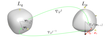
Figure 3: Illustration of the case $W=1$ for the ${\mathcal{B}}_{q}(W)$-update: all classifiers and image via $\nabla{\varphi^{\dagger}}$ belong to a ball of radius 1 (here, $q=3$, $p=3/2$).

Proof of Lemma 5.

We start by the sphere. Let $\varphi(\bm{x})\stackrel{{\scriptstyle\mathrm{.}}}{{=}}(1/2)\cdot\|\bm{x}\|_{2}^{2}$. Since a Bregman divergence is invariant to linear transformation, it comes from Table 7 that

$$D_{\varphi}\left(\frac{\bm{x}^{S}}{g_{S}(\bm{x}^{S})}\bigm{\|}\frac{\bm{c}^{S}}{g_{S}(\bm{c}^{S})}\right)=\frac{1}{g_{S}(\bm{c}^{S})}\cdot D_{\varphi^{\dagger}}(\bm{x}\|\bm{c})=1-\cos D_{G}(\bm{x},\bm{c}),$$

where we recall that $D_{G}$ denotes the geodesic distance on the sphere (see Figure 1 and Appendix C). Equivalently,

$$\left\|\frac{1}{g_{S}(\bm{x}^{S})}\cdot\bm{x}^{S}-\frac{1}{g_{S}(\bm{c}^{S})}\cdot\bm{c}^{S}\right\|_{2}^{2} = 1-\cos D_{G}(\bm{x},\bm{c})\>\>.$$ (57)

This equality allows us to use $k$-means++ using the LHS of (57) to compute the distribution that picks a center. The key to using the approximation property of $k$-means++ relies on the existence of a coordinate system on the sphere for which the cluster centroid is just the average of the cluster points (polar coordinates), an average that eventually has to be rescaled if the coordinate system is not that one [Dhillon and Modha, 2001, Endo and Miyamoto, 2015]. The existence of this coordinate system makes that the proof of Arthur and Vassilvitskii [2007] (and in particular the key Lemmata 3.2 and 3.3) can be carried out without modification to yield the same approximation ratio as that of Arthur and Vassilvitskii [2007] if the distortion at hand is the squared Euclidean distance, which turns out to be $D_{\mathrm{rec}}(.:.)$ from eq. (57).
The case of the hyperboloid follows the exact same path, but starts from the fact that Table 7 now brings

$$D_{\varphi}\left(\frac{\bm{x}^{H}}{g_{H}(\bm{x}^{H})}\bigm{\|}\frac{\bm{c}^{H}}{g_{H}(\bm{c}^{H})}\right)=\cosh D_{G}(\bm{y},\bm{c})-1=\left\|\frac{1}{g_{H}(\bm{x}^{H})}\cdot\bm{x}^{H}-\frac{1}{g_{H}(\bm{c}^{H})}\cdot\bm{c}^{H}\right\|_{2}^{2}\>\>.$$

To finish, in the same way as for the Sphere, we just need the existence of a coordinate system for which the centroid is an average of the cluster points, which can be obtained from hyperbolic barycentric coordinates [Ungar, 2014, Section 18]. ∎

Appendix C Working out examples of Table 7

We fill in the details justifying each of the examples of Equation 3 provided in Table 2. We also provide the form of the corresponding divergences $D_{\varphi}$ and distortions $D_{\varphi^{\dagger}}$ in the augmented Table 7.

	$\varphi$	$D_{\varphi}\left(\bm{x}\|\bm{y}\right)$	$g$	$\varphi^{\dagger}$	$D_{\varphi^{\dagger}}\left(\bm{x}\|\bm{y}\right)$
I	$\frac{1}{2}\cdot(1+\|\bm{x}\|_{2}^{2})$	$(1/2)\cdot\|\bm{x}-\bm{y}\|_{2}^{2}$	$\|\bm{x}\|_{2}$	$\|\bm{x}\|_{2}$	$\|\bm{x}\|_{2}\cdot\left(1-\cos\angle\bm{x},\bm{y}\right)$
II	$\frac{1}{2}\cdot(W+\|\bm{x}\|_{q}^{2})$	$(1/2)\cdot(\|\bm{x}\|_{q}^{2}-\|\bm{y}\|_{q}^{2})$	$\frac{\|\bm{x}\|_{q}}{W}$	$W\cdot\|\bm{x}\|_{q}$	$W\cdot|\bm{x}\|_{q}-W\cdot\sum_{i}\frac{x_{i}\cdot\mathrm{sign}(y_{i})\cdot|y_{i}|^{q-1}}{\|\bm{y}\|_{q}^{q-1}}$
		$-\sum_{i}\frac{(x_{i}-y_{i})\cdot\mathrm{sign}(y_{i})\cdot|y_{i}|^{q-1}}{\|\bm{y}\|_{q}^{q-2}}$
III	$\frac{1}{2}\cdot(u^{2}+\|\bm{x}^{S}\|_{2}^{2})$	$(1/2)\cdot\|\bm{x}^{S}-\bm{y}^{S}\|_{2}^{2}$	$\frac{\|\bm{x}\|_{2}}{\sin\|\bm{x}\|_{2}}$	$\|\bm{x}^{S}\|_{2}$	$\frac{\|\bm{x}\|_{2}}{\sin\|\bm{x}\|_{2}}\cdot\left(1-\cos D_{G}(\bm{x},\bm{y})\right)$
IV	$\frac{1}{2}\cdot(u^{2}+\|\bm{x}^{H}\|_{2}^{2})$	$(1/2)\cdot\|\bm{x}^{H}-\bm{y}^{H}\|_{2}^{2}$	$-\frac{\|\bm{x}\|_{2}}{\sinh\|\bm{x}\|_{2}}$	$\|\bm{x}^{H}\|_{2}$	$-\frac{\|\bm{x}\|_{2}}{\sinh\|\bm{x}\|_{2}}\cdot\left(\cosh D_{G}(\bm{x},\bm{y})-1\right)$
V	$\sum_{i}x_{i}\log x_{i}-x_{i}$	$\sum_{i}x_{i}\log\frac{x_{i}}{y_{i}}$	$\bm{1}^{\top}\bm{x}$	$\sum_{i}x_{i}\log x_{i}-\bm{1}^{\top}\bm{x}$	$\sum_{i}x_{i}\log\frac{x_{i}}{y_{i}}$
		$-\bm{1}^{\top}(\bm{x}-\bm{y})$		$-(\bm{1}^{\top}\bm{x})\log(\bm{1}^{\top}\bm{x})$	$-d\cdot\mathbb{E}[\mathsf{X}]\cdot\log\frac{\mathbb{E}[\mathsf{X}]}{\mathbb{E}[\mathsf{Y}]}$
VI	$-d-\sum_{i}\log x_{i}$	$\sum_{i}\frac{x_{i}}{y_{i}}$	$\prod_{i}x_{i}^{1/d}$	$-d\cdot\prod_{i}x_{i}^{1/d}$	$\sum_{i}\frac{x_{i}(\pi_{\bm{y}})^{1/d}}{y_{i}}-d(\pi_{\bm{x}})^{1/d}$
		$-\sum_{i}\log\frac{x_{i}}{y_{i}}-d$
VII	$\mathrm{tr}\left(\mbox{{\small{x}}}\log\mbox{{\small{x}}}-\mbox{{\small{x}}}\right)$	$\mathrm{tr}\left(\mbox{{\small{x}}}\log\mbox{{\small{x}}}-\mbox{{\small{x}}}\log\mbox{{\small{y}}}\right)$	$\mathrm{tr}\left(\mbox{{\small{x}}}\right)$	$\mathrm{tr}\left(\mbox{{\small{x}}}\log\mbox{{\small{x}}}-\mbox{{\small{x}}}\right)$	$\mathrm{tr}\left(\mbox{{\small{x}}}\log\mbox{{\small{x}}}-\mbox{{\small{x}}}\log\mbox{{\small{y}}}\right)$
		$-\mathrm{tr}\left(\mbox{{\small{x}}}\right)+\mathrm{tr}\left(\mbox{{\small{y}}}\right)$		$-\mathrm{tr}\left(\mbox{{\small{x}}}\right)\log\mathrm{tr}\left(\mbox{{\small{x}}}\right)$	$-\mathrm{tr}\left(\mbox{{\small{x}}}\right)\cdot\log\frac{\mathrm{tr}\left(\mbox{{\small{x}}}\right)}{\mathrm{tr}\left(\mbox{{\small{y}}}\right)}$
VIII	$-d-\log\det(\mbox{{\small{x}}})$	$\mathrm{tr}\left(\mbox{{\small{x}}}\mbox{{\small{y}}}^{-1}\right)$	$\det(\mbox{{\small{x}}}^{1/d})$	$-d\cdot\det(\mbox{{\small{x}}}^{1/d})$	$\det(\mbox{{\small{y}}}^{1/d})\mathrm{tr}\left(\mbox{{\small{x}}}\mbox{{\small{y}}}^{-1}\right)-d\cdot\det(\mbox{{\small{x}}}^{1/d})$
		$-\log\det(\mbox{{\small{x}}}\mbox{{\small{y}}}^{-1})-d$

Table 7: Example of distortions (right columns) that can be “reverse engineered” as Bregman divergences involving a particular, non necessary linear $g$. Function $\bm{x}^{S}\stackrel{{\scriptstyle\mathrm{.}}}{{=}}f(\bm{x}):{\mathbb{R}}^{d}\rightarrow{\mathbb{R}}^{d+1}$ is the (S)phere lifting map defined in (69), and $\bm{x}^{H}$ is the (H)yperboloid lifting map defined in (80). $D_{G}(.,.)$ is the geodesic distance between the exponential map of $\bm{x}$ and $\bm{y}$ on their respective manifold (sphere or hyperboloid). Related proofs are in Section C. Expectation $\mathbb{E}[\mathsf{X}]$ is a shorthand for $(1/d)\cdot\sum_{i}x_{i}$. $W\in\mathbb{R}_{+*}$ and $u\in\mathbb{R}$ are constants.

Row I —

for $\mathcal{X}=\mathbb{R}^{d}$, consider $\varphi(\bm{x})=(1+\|\bm{x}\|_{2}^{2})/2$ and $g(\bm{x})=\|\bm{x}\|_{2}$ (we project on the Euclidean sphere). It comes

$$\varphi^{\dagger}(\bm{x}) = \|\bm{x}\|_{2}\cdot\left(\frac{1+\left\|\frac{1}{\|\bm{x}\|_{2}}\cdot\bm{x}\right\|_{2}^{2}}{2}\right)=\|\bm{x}\|_{2}\>\>.$$ (58)

$g$ is not linear (but it is homogeneous of degree 1), but we have

$$\varphi(\bm{x})=1=\bm{x}^{\top}\nabla\varphi(\bm{x})\>\>,\forall\bm{x}:\|\bm{x}\|_{2}=1\>\>,$$ (59)

so $\varphi$ is 1-homogeneous on the Euclidean sphere, and we can apply Theorem 1. We have

$$g(\bm{x})\cdot D_{\varphi}\left(\frac{1}{g(\bm{x})}\cdot\bm{x}\|\frac{1}{g(\bm{y})}\cdot\bm{y}\right) = \frac{\|\bm{x}\|_{2}}{2}\cdot\left\|\frac{1}{\|\bm{x}\|_{2}}\cdot\bm{x}-\frac{1}{\|\bm{y}\|_{2}}\cdot\bm{y}\right\|_{2}^{2}$$ (60)

$$= \|\bm{x}\|_{2}\cdot\left(1-\frac{\bm{x}^{\top}\bm{y}}{\|\bm{x}\|_{2}\|\bm{y}\|_{2}}\right)=\|\bm{x}\|_{2}\cdot(1-\cos(\bm{x},\bm{y}))\>\>,$$

and we also have

$$D_{\varphi^{\dagger}}\left(\bm{x}\|\bm{y}\right) = \|\bm{x}\|_{2}-\|\bm{y}\|_{2}-\frac{1}{\|\bm{y}\|_{2}}\cdot(\bm{x}-\bm{y})^{\top}\bm{y}$$ (61)

$$= \|\bm{x}\|_{2}-\|\bm{y}\|_{2}-\frac{\bm{x}^{\top}\bm{y}}{\|\bm{y}\|_{2}}+\|\bm{y}\|_{2}$$

$$= \|\bm{x}\|_{2}\cdot\left(1-\frac{\bm{x}^{\top}\bm{y}}{\|\bm{x}\|_{2}\|\bm{y}\|_{2}}\right)=\|\bm{x}\|_{2}\cdot(1-\cos(\bm{x},\bm{y}))\>\>,$$ (62)

which is equal to Equation (60), so we check that Theorem 1 applies in this case. $D_{\varphi^{\dagger}}$ has some properties. One is a weak form of triangle inequality.

Lemma 16

$D_{\varphi^{\dagger}}\left(\bm{x}\|\bm{y}\right)+D_{\varphi^{\dagger}}\left(\bm{y}\|\bm{z}\right)\leq D_{\varphi^{\dagger}}\left(\bm{x}\|\bm{z}\right)$, $\forall\bm{x},\bm{y},\bm{z}$ such that $\|\bm{y}\|_{2}\leq\|\bm{x}\|_{2}$.

Proof.

$$D_{\varphi^{\dagger}}\left(\bm{x}\|\bm{y}\right)+D_{\varphi^{\dagger}}\left(\bm{y}\|\bm{z}\right)$$ (63)

$$= \|\bm{x}\|_{2}\cdot(1-\cos(\bm{x},\bm{y}))+\|\bm{y}\|_{2}\cdot(1-\cos(\bm{y},\bm{z}))$$

$$= \|\bm{x}\|_{2}\cdot\left((1-\cos(\bm{x},\bm{y}))+(1-\cos(\bm{y},\bm{z}))\right)+(\|\bm{y}\|_{2}-\|\bm{x}\|_{2})\cdot(1-\cos(\bm{y},\bm{z}))$$

$$\leq \|\bm{x}\|_{2}\cdot(1-\cos(\bm{x},\bm{z}))+(\|\bm{y}\|_{2}-\|\bm{x}\|_{2})\cdot(1-\cos(\bm{y},\bm{z}))$$

$$\leq D_{\varphi^{\dagger}}\left(\bm{x}\|\bm{z}\right)+(\|\bm{y}\|_{2}-\|\bm{x}\|_{2})\cdot(1-\cos(\bm{y},\bm{z}))$$

$$\leq D_{\varphi^{\dagger}}\left(\bm{x}\|\bm{z}\right)\>\>,$$

since $\|\bm{y}\|_{2}\leq\|\bm{x}\|_{2}$. We have used the fact that $(1-\cos(\bm{x},\bm{y}))$ is half the Euclidean distance between unit-normalized vectors. ∎

It turns out that $D_{\varphi^{\dagger}}(\bm{x}\|\bm{\mu})$ can be related to the log-likelihood of a von Mises-Fisher distribution with expected direction $\bm{\mu}$, which is useful in text analysis [Reisinger et al., 2010].

Row II —

Let $\varphi(\bm{x})\stackrel{{\scriptstyle\mathrm{.}}}{{=}}(1/2)\cdot(u^{2}+\|\bm{x}\|_{q}^{2})$, for $q>1$ [Kivinen et al., 2006]. We have

$$\varphi\left(\frac{1}{g(\bm{x})}\cdot\bm{x}\right) = \frac{u^{2}}{2}+\frac{1}{2}\cdot\left\|\frac{1}{g(\bm{x})}\cdot\bm{x}\right\|_{q}^{2}=\frac{u^{2}}{2}+\frac{1}{2g^{2}(\bm{x})}\cdot\|\bm{x}\|_{q}^{2}\>\>.$$ (64)

We also have

$$\left(\frac{1}{g(\bm{x})}\cdot\bm{x}\right)^{\top}\nabla\varphi\left(\frac{1}{g(\bm{x})}\cdot\bm{x}\right) = \frac{1}{g(\bm{x})}\cdot\sum_{i}\frac{x_{i}\cdot\mathrm{sign}\left(\frac{1}{g(\bm{x})}\cdot x_{i}\right)\left|\frac{1}{g(\bm{x})}\cdot x_{i}\right|^{q-1}}{\left\|\frac{1}{g(\bm{x})}\cdot\bm{x}\right\|_{q}^{q-2}}$$ (65)

$$= \sum_{i}\frac{\left|\frac{1}{g(\bm{x})}\cdot x_{i}\right|^{q}}{\left\|\frac{1}{g(\bm{x})}\cdot\bm{x}\right\|_{q}^{q-2}}$$

$$= \frac{1}{g^{2}(\bm{x})}\cdot\|\bm{x}\|_{q}^{2}\>\>.$$

To have the condition of Theorem 1 satisfied, we therefore need

$$\|\bm{x}\|_{q} = ug(\bm{x})\>\>,$$ (66)

So we use $g(\bm{x})=\|\bm{x}\|_{q}/W$ and $u=W$, observing that $\varphi$ is 1-homogeneous on the $L_{p}$ sphere. We check that

$$\varphi^{\dagger}(\bm{x}) = W\cdot\|\bm{x}\|_{q}\>\>.$$ (67)

and we obtain

$$D_{\varphi^{\dagger}}(\bm{w}\|\bm{w}^{\prime}) = W\cdot\|\bm{w}\|_{q}-W\cdot\sum_{i}\frac{w_{i}\cdot\mathrm{sign}(w^{\prime}_{i})\cdot|w^{\prime}_{i}|^{q-1}}{\|\bm{w}^{\prime}\|_{q}^{q-1}}\>\>.$$ (68)

Row III —

As in Buss and Fillmore [2001], we assume $\|\bm{x}\|_{2}\leq\pi$, or we renormalize or change the radius of the ball) We first lift the data points using the Sphere lifting map $\mathbb{R}^{d}\ni\bm{x}\mapsto\bm{x}^{S}\in\mathbb{R}^{d+1}$:

$$\bm{x}^{S} \stackrel{{\scriptstyle\mathrm{.}}}{{=}} [x_{1}\quad x_{2}\quad\cdots\quad x_{d}\quad r_{\bm{x}}\cot r_{\bm{x}}]^{\top}\>\>,$$ (69)

where $r_{\bm{x}}\stackrel{{\scriptstyle\mathrm{.}}}{{=}}\|\bm{x}\|_{2}$ is the Euclidean norm of $\bm{x}$. Notice that the last coordinate is a coordinate of the Hessian of the geodesic distance to the origin on the sphere [Buss and Fillmore, 2001]. We then let $g(\bm{x}^{S})\stackrel{{\scriptstyle\mathrm{.}}}{{=}}r_{\bm{x}}/\sin r_{\bm{x}}$ (notice that $g$ is computed uding the first $d$ coordinates). Finally, for $\mathcal{X}=\mathbb{R}^{d+1}$ and $u>1$, consider $\varphi(\bm{x}^{S})=(u^{2}+\|\bm{x}^{S}\|_{2}^{2})/2$. The set of points for which $\varphi(\bm{x}^{S})=(\bm{x}^{S})^{\top}\nabla\varphi(\bm{x}^{S})$ is equivalently the subset $\mathcal{X}_{g}\subseteq\mathbb{R}^{d+1}$ such that

$$\mathcal{X}_{g} \stackrel{{\scriptstyle\mathrm{.}}}{{=}} \{\bm{x}^{S}:g^{2}(\bm{x}^{S})=u^{2}\}\>\>.$$ (70)

So $\varphi$ satisfies the restricted positive homogeneity of degree 1 on $\mathcal{X}_{g}$ and we can apply Theorem 1. We first remark that:

$$\|\bm{x}^{S}\|_{2}^{2} = r^{2}_{\bm{x}}+r^{2}_{\bm{x}}\cot^{2}r_{\bm{x}}$$ (71)

$$= \frac{r^{2}_{\bm{x}}}{\sin r^{2}_{\bm{x}}}=g^{2}(\bm{x}^{S})\>\>,$$

and

$$\varphi^{\dagger}(\bm{x}^{S}) = \frac{r_{\bm{x}}}{\sin r_{\bm{x}}}\cdot\varphi\left(\frac{\sin r_{\bm{x}}}{r_{\bm{x}}}\cdot\bm{x}^{S}\right)=\frac{r_{\bm{x}}}{\sin r_{\bm{x}}}\cdot\left(\frac{\sin r_{\bm{x}}}{r_{\bm{x}}}\right)^{2}\cdot\|\bm{x}^{S}\|_{2}^{2}=\|\bm{x}^{S}\|_{2}\>\>,$$ (72)

and finally, because of the spherical law of cosines,

$$\sin r_{\bm{x}}\sin r_{\bm{y}}\cos(\bm{x},\bm{y})+\cos r_{\bm{x}}\cos r_{\bm{y}} = \cos D_{G}(\bm{x},\bm{y})\>\>,$$ (73)

where we recall from eq. (18) that $D_{G}(\bm{x},\bm{y})$ is the geodesic distance between the image of the exponential maps of $\bm{x}$ and $\bm{y}$ on the sphere.

We then derive

$$g(\bm{x}^{S})\cdot D_{\varphi}\left(\frac{1}{g(\bm{x}^{S})}\cdot\bm{x}^{S}\|\frac{1}{g(\bm{y}^{S})}\cdot\bm{y}^{S}\right)$$ (74)

$$= \frac{r_{\bm{x}}}{2\sin r_{\bm{x}}}\cdot\left\|\frac{\sin r_{\bm{x}}}{r_{\bm{x}}}\cdot\bm{x}^{S}-\frac{\sin r_{\bm{y}}}{r_{\bm{y}}}\cdot\bm{y}^{S}\right\|_{2}^{2}$$

$$= \frac{r_{\bm{x}}}{2\sin r_{\bm{x}}}\cdot\left(\frac{\sin^{2}r_{\bm{x}}}{\|\bm{x}\|^{2}_{2}}\cdot\|\bm{x}^{S}\|_{2}^{2}+\frac{\sin^{2}r_{\bm{y}}}{\|\bm{y}\|^{2}_{2}}\cdot\|\bm{y}^{S}\|_{2}^{2}-2\cdot\frac{\sin r_{\bm{x}}}{r_{\bm{x}}}\cdot\frac{\sin r_{\bm{y}}}{r_{\bm{y}}}\cdot(\bm{x}^{S})^{\top}\bm{y}^{S}\right)$$

$$= \frac{r_{\bm{x}}}{\sin r_{\bm{x}}}\cdot\left(1-\frac{\sin r_{\bm{x}}}{r_{\bm{x}}}\cdot\frac{\sin r_{\bm{y}}}{r_{\bm{y}}}\cdot(\bm{x}^{S})^{\top}\bm{y}^{S}\right)$$

$$= \frac{r_{\bm{x}}}{\sin r_{\bm{x}}}\cdot\left(1-\frac{\sin r_{\bm{x}}}{r_{\bm{x}}}\cdot\frac{\sin r_{\bm{y}}}{r_{\bm{y}}}\cdot\left(\bm{x}^{\top}\bm{y}+r_{\bm{x}}r_{\bm{y}}\cot r_{\bm{x}}\cot r_{\bm{y}}\right)\right)$$

$$= \frac{r_{\bm{x}}}{\sin r_{\bm{x}}}\cdot\left(1-\sin r_{\bm{x}}\sin r_{\bm{y}}\cdot\left(\cos(\bm{x},\bm{y})+\cot r_{\bm{x}}\cot r_{\bm{y}}\right)\right)$$

$$= \frac{r_{\bm{x}}}{\sin r_{\bm{x}}}\cdot\left(1-\left(\sin r_{\bm{x}}\sin r_{\bm{y}}\cos(\bm{x},\bm{y})+\cos r_{\bm{x}}\cos r_{\bm{y}}\right)\right)$$

$$= \frac{r_{\bm{x}}}{\sin r_{\bm{x}}}\cdot\left(1-\cos D_{G}(\bm{x},\bm{y})\right)\>\>.$$ (76)

In Equation (74), we use Equation (71), and we use Equation (73) in Equation (76). We also check

$$D_{\varphi^{\dagger}}(\bm{x}^{S}\|\bm{y}^{S}) = \|\bm{x}^{S}\|_{2}-\|\bm{y}^{S}\|_{2}-\frac{1}{\|\bm{y}^{S}\|_{2}}\cdot(\bm{x}^{S}-\bm{y}^{S})^{\top}\bm{y}^{S}$$ (77)

$$= \|\bm{x}^{S}\|_{2}-\frac{1}{\|\bm{y}^{S}\|_{2}}\cdot(\bm{x}^{S})^{\top}\bm{y}^{S}$$

$$= \|\bm{x}^{S}\|_{2}\cdot\left(1-\frac{(\bm{x}^{S})^{\top}\bm{y}^{S}}{\|\bm{x}^{S}\|_{2}\|\bm{y}^{S}\|_{2}}\right)$$

$$= \frac{r_{\bm{x}}}{\sin r_{\bm{x}}}\cdot\left(1-\cos D_{G}(\bm{x},\bm{y})\right)\>\>.$$ (78)

To obtain (78), we use the fact that

$$\frac{(\bm{x}^{S})^{\top}\bm{y}^{S}}{\|\bm{x}^{S}\|_{2}\|\bm{y}^{S}\|_{2}} = \frac{\sin r_{\bm{x}}}{r_{\bm{x}}}\cdot\frac{\sin r_{\bm{y}}}{r_{\bm{y}}}\cdot\left(\bm{x}^{\top}\bm{y}+r_{\bm{x}}r_{\bm{y}}\cot r_{\bm{x}}\cot r_{\bm{y}}\right)\>\>,$$ (79)

and then plug it into Equation (78), which yields the identity between Equation (C) (and thus (76)) and (78). So Theorem 1 holds in this case as well.

We remark that $(1/g(\bm{x}^{S}))\cdot\bm{x}^{S}=\exp_{\bm{0}}(\bm{x})$ is the exponential map for the sphere [Buss and Fillmore, 2001].

Row IV —

In the same way as we did for row IV, we first create a lifting map, but this time complex valued, the Hyperboloid lifting map $H$: $\mathbb{R}^{d}\ni\bm{x}\mapsto\bm{x}^{H}\in\mathbb{R}^{d}\times\mathbb{C}$. With an abuse of notation, it is given by

$$\bm{x}^{H} \stackrel{{\scriptstyle\mathrm{.}}}{{=}} [x_{1}\quad x_{2}\quad\cdots\quad x_{d}\quad ir_{\bm{x}}\coth r_{\bm{x}}]^{\top}\>\>,$$ (80)

and we let $g(\bm{x}^{H})\stackrel{{\scriptstyle\mathrm{.}}}{{=}}-r_{\bm{x}}/\sinh r_{\bm{x}}$, with $\coth$ and $\sinh$ defining respectively the hyperbolic cotangent and hyperbolic sine. We let $0\coth 0=0/\sinh 0=1$. Notice that the complex number is pure imaginary and so $H$ defines a $d$ dimensional manifold that lives in $\mathbb{R}^{d+1}$ assuming that the last coordinate is the imaginary axis. Let $\exp_{\bm{q}}(\bm{x})\stackrel{{\scriptstyle\mathrm{.}}}{{=}}(1/g(\bm{x}^{H})\cdot\bm{x}^{H}$. Notice that

$$\left\|\exp_{\bm{q}}(\bm{x})\right\|_{2}^{2} = \frac{\sinh^{2}r_{\bm{x}}}{r^{2}_{\bm{x}}}\cdot\left(r^{2}_{\bm{x}}+i^{2}r^{2}_{\bm{x}}\coth^{2}r_{\bm{x}}\right)$$ (81)

$$= \sinh^{2}r_{\bm{x}}+i^{2}\cosh^{2}r_{\bm{x}}$$

$$= \sinh^{2}r_{\bm{x}}-\cosh^{2}r_{\bm{x}}=-1\>\>,$$

so $\exp_{\bm{q}}(\bm{x})$ defines a lifting map from ${\mathbb{R}}^{d}$ to the hyperboloid model $\mathbb{H}^{d}$ of hyperbolic geomety Galperin [1993]. In fact, it defines the exponential map for the plane $T_{\bm{q}}\mathbb{H}^{d}$ tangent to $\mathbb{H}^{d}$ in point $\bm{q}\stackrel{{\scriptstyle\mathrm{.}}}{{=}}[0\quad 0\quad\cdots\quad 0\quad i]=\bm{0}^{H}$. To see this, remark that we can express the geodesic distance $D_{G}$ with the hyperbolic metric between $\bm{x}^{H}$ and $\bm{y}^{H}$ as

$$D_{G}(\bm{x}^{H},\bm{y}^{H}) \stackrel{{\scriptstyle\mathrm{.}}}{{=}} \cosh^{-1}(-(\bm{x}^{H})^{\top}\bm{y}^{H})\>\>,$$ (82)

where $\cosh^{-1}$ is the inverse hyperbolic cosine. So, for any $\bm{x}\in T_{\bm{q}}\mathbb{H}^{d}$, since $r_{\bm{x}}=\|\bm{x}-\bm{0}\|_{2}$, we have

$$D_{G}(\exp_{\bm{q}}(\bm{x}),\bm{q}) = \cosh^{-1}(-(\bm{x}^{H})^{\top}\bm{0}^{H})$$ (83)

$$= \cosh^{-1}(-i^{2}\cosh r_{\bm{x}})$$

$$= r_{\bm{x}}=\|\bm{x}-\bm{0}\|_{2}\>\>,$$

and $\exp_{\bm{q}}(\bm{x})$ is indeed the exponential map for $T_{\bm{q}}\mathbb{H}^{d}$. Now, remark that

$$\exp_{\bm{q}}(\bm{x})^{\top}\exp_{\bm{q}}(\bm{y}) = \frac{\sinh r_{\bm{x}}}{r_{\bm{x}}}\cdot\frac{\sinh r_{\bm{y}}}{r_{\bm{y}}}\cdot(\bm{x}^{H})^{\top}\bm{y}^{H}$$ (84)

$$= \frac{\sinh r_{\bm{x}}}{r_{\bm{x}}}\cdot\frac{\sinh r_{\bm{y}}}{r_{\bm{y}}}\cdot\left(\bm{x}^{\top}\bm{y}+i^{2}r_{\bm{x}}r_{\bm{y}}\coth r_{\bm{x}}\coth r_{\bm{y}}\right)$$

$$= \sinh r_{\bm{x}}\sinh r_{\bm{y}}\cdot\left(\cos(\bm{x},\bm{y})-\coth r_{\bm{x}}\coth r_{\bm{y}}\right)$$

$$= \sinh r_{\bm{x}}\sinh r_{\bm{y}}\cos(\bm{x},\bm{y})-\cosh r_{\bm{x}}\cosh r_{\bm{y}}$$

$$= -\cosh D_{G}(\bm{x}^{H},\bm{y}^{H})\>\>.$$

Eq. (84) holds by the hyperbolic law of cosines. Now, we let $\varphi(\bm{x}^{H})=(u^{2}+\|\bm{x}^{H}\|_{2}^{2})/2$ and

$$\mathcal{X}_{g} \stackrel{{\scriptstyle\mathrm{.}}}{{=}} \{\bm{x}^{H}:\|\bm{x}^{H}\|_{2}^{2}=u^{2}\}\>\>.$$ (85)

We check that $\varphi(\bm{x}^{H})=u^{2}=(\bm{x}^{H})^{\top}\nabla\varphi(\bm{x}^{H})$ for any $\bm{x}^{H}\in\mathcal{X}_{g}$, so we can apply Theorem 1. We then use eqs. (81) and (84) and derive

$$g(\bm{x}^{H})\cdot D_{\varphi}\left(\frac{1}{g(\bm{x}^{H})}\cdot\bm{x}^{H}\|\frac{1}{g(\bm{y}^{H})}\cdot\bm{y}^{H}\right)$$ (86)

$$= -\frac{r_{\bm{x}}}{2\sinh r_{\bm{x}}}\cdot\left\|\exp_{\bm{q}}(\bm{x})-\exp_{\bm{q}}(\bm{y})\right\|_{2}^{2}$$

$$= -\frac{r_{\bm{x}}}{2\sinh r_{\bm{x}}}\cdot\left(\left\|\exp_{\bm{q}}(\bm{x})\right\|_{2}^{2}+\left\|\exp_{\bm{q}}(\bm{y})\right\|_{2}^{2}-2\exp_{\bm{q}}(\bm{x})^{\top}\exp_{\bm{q}}(\bm{y})\right)$$

$$= -\frac{r_{\bm{x}}}{\sinh r_{\bm{x}}}\cdot\left(\cosh D_{G}(\bm{x}^{H},\bm{y}^{H})-1\right)\>\>.$$

Note that eq. (86) is a negative-valued and concave distortion.

Row V —

for $\mathcal{X}=\mathbb{R}_{+*}^{d}$, consider $\varphi(\bm{x})=\sum_{i}x_{i}\log x_{i}-x_{i}$ and $g(\bm{x})=\bm{1}^{\top}\bm{x}$ (we normalize on the simplex). Since $g$ is linear, we do not need to check for the homogeneity of $\varphi$, and we directly obtain:

$$g(\bm{x})\cdot D_{\varphi}\left(\frac{1}{g(\bm{x})}\cdot\bm{x}\|\frac{1}{g(\bm{y})}\cdot\bm{y}\right) = \sum_{i}x_{i}\log x_{i}-(\bm{1}^{\top}\bm{x})\log(\bm{1}^{\top}\bm{x})-\bm{1}^{\top}\bm{x}$$ (87)

$$-\frac{\bm{1}^{\top}\bm{x}}{\bm{1}^{\top}\bm{y}}\cdot\sum_{i}y_{i}\log y_{i}-(\bm{1}^{\top}\bm{x})\log(\bm{1}^{\top}\bm{y})+\bm{1}^{\top}\bm{x}$$

$$-(\bm{1}^{\top}\bm{x})\cdot\sum_{i}\left(\frac{x_{i}}{\bm{1}^{\top}\bm{x}}-\frac{y_{i}}{\bm{1}^{\top}\bm{y}}\right)\cdot\log\frac{y_{i}}{\bm{1}^{\top}\bm{y}}$$

$$= \sum_{i}x_{i}\log\frac{x_{i}}{y_{i}}-(\bm{1}^{\top}\bm{x})\cdot\log\frac{\bm{1}^{\top}\bm{x}}{\bm{1}^{\top}\bm{y}}\>\>.$$

Furthermore,

$$\varphi^{\dagger}(\bm{x}) = \bm{1}^{\top}\bm{x}\cdot\left(\sum_{i}\frac{x_{i}}{\bm{1}^{\top}\bm{x}}\cdot\log\frac{x_{i}}{\bm{1}^{\top}\bm{x}}-1\right)=\sum_{i}x_{i}\log x_{i}-(\bm{1}^{\top}\bm{x})\log(\bm{1}^{\top}\bm{x})-\bm{1}^{\top}\bm{x}\>\>.$$ (88)

Noting that $\varphi^{\dagger}(\bm{x})$ is the sum of three terms, one of which is linear and can be removed for the divergence, so the divergence is just the sum of the two divergences with the two generators, which is found to be Equation (87) as well. Remark that while the KL divergence is convex in its both arguments, $D_{\varphi^{\dagger}}(\bm{x}\|\bm{y})$ may not be (jointly) convex. Indeed, its Hessian in $\bm{y}$ equals:

$$\mbox{{\small{H}}}_{\bm{y}}(D_{\varphi^{\dagger}}) = \mathrm{Diag}(\{x_{i}/y_{i}^{2}\}_{i})-\frac{\bm{1}^{\top}\bm{x}}{(\bm{1}^{\top}\bm{y})^{2}}\cdot\bm{1}\bm{1}^{\top}\>\>,$$ (89)

which may be indefinite.

Row VI —

for $\mathcal{X}=\mathbb{R}_{+*}^{d}$, consider $\varphi(\bm{x})=-d-\sum_{i}\log x_{i}$ and $g(\bm{x})=(\pi_{\bm{x}})^{1/d}$, where we let $\pi_{\bm{x}}\stackrel{{\scriptstyle\mathrm{.}}}{{=}}\prod_{i}x_{i}$ (we normalize with the geometric average). It comes

$$\varphi^{\dagger}(\bm{x}) = (\pi_{\bm{x}})^{1/d}\cdot\left(-d-\sum_{i}\log\frac{x_{i}}{(\pi_{\bm{x}})^{1/d}}\right)=-d\cdot(\pi_{\bm{x}})^{1/d}\>\>.$$ (90)

$g$ is not linear (but it is homogeneous of degree $1$), and we have

$$\varphi(\bm{x})=-d=\bm{x}^{\top}\nabla\varphi(\bm{x})\>\>,\forall\bm{x}:\prod_{i}x_{i}=1\>\>,$$ (91)

so $\varphi$ is 1-homogeneous on $\mathcal{X}_{g}$, and we can apply Theorem 1. We have

$$g(\bm{x})\cdot D_{\varphi}\left(\frac{1}{g(\bm{x})}\cdot\bm{x}\|\frac{1}{g(\bm{y})}\cdot\bm{y}\right)$$ (92)

$$= (\pi_{\bm{x}})^{1/d}\cdot\sum_{i}\left(\frac{x_{i}(\pi_{\bm{y}})^{1/d}}{y_{i}(\pi_{\bm{x}})^{1/d}}-\log\frac{x_{i}(\pi_{\bm{y}})^{1/d}}{y_{i}(\pi_{\bm{x}})^{1/d}}\right)-d(\pi_{\bm{x}})^{1/d}$$

$$= \sum_{i}\frac{x_{i}(\pi_{\bm{y}})^{1/d}}{y_{i}}-d(\pi_{\bm{x}})^{1/d}\log(\pi_{\bm{x}})^{1/d}-(\pi_{\bm{x}})^{1/d}\log\pi_{\bm{y}}+(\pi_{\bm{x}})^{1/d}\log\pi_{\bm{y}}$$

$$+d(\pi_{\bm{x}})^{1/d}\log(\pi_{\bm{x}})^{1/d}-d(\pi_{\bm{x}})^{1/d}$$

$$= \sum_{i}\frac{x_{i}(\pi_{\bm{y}})^{1/d}}{y_{i}}-d(\pi_{\bm{x}})^{1/d}\>\>.$$

We also have

$$\frac{\partial}{\partial x_{i}}\varphi^{\dagger}(\bm{x}) = -(1/x_{i})\cdot(\pi_{\bm{x}})^{1/d}\>\>,$$ (93)

and so

$$D_{\varphi^{\dagger}}\left(\bm{x}\|\bm{y}\right) = -d(\pi_{\bm{x}})^{1/d}+d(\pi_{\bm{y}})^{1/d}+\cdot\sum_{i}(x_{i}-y_{i})\cdot\frac{(\pi_{\bm{y}})^{1/d}}{y_{i}}$$ (94)

$$= -d(\pi_{\bm{x}})^{1/d}+d(\pi_{\bm{y}})^{1/d}+\sum_{i}\frac{x_{i}(\pi_{\bm{y}})^{1/d}}{y_{i}}-d(\pi_{\bm{y}})^{1/d}$$

$$= \sum_{i}\frac{x_{i}(\pi_{\bm{y}})^{1/d}}{y_{i}}-d(\pi_{\bm{x}})^{1/d}\>\>,$$

which is equal to Equation (92), so we check that Theorem 1 applies in this case.

Row VII —

We use the following fact Kulis et al. [2009]. Let $\mbox{{\small{x}}}=\mbox{{\small{u}}}\mbox{{\small{l}}}\mbox{{\small{u}}}^{\top}$ and $\mbox{{\small{y}}}=\mbox{{\small{v}}}\mbox{{\small{t}}}\mbox{{\small{v}}}^{\top}$ be the eigendecomposition of symmetric positive definite matrices x and y, with $\mbox{{\small{l}}}\stackrel{{\scriptstyle\mathrm{.}}}{{=}}\mathrm{Diag}(\bm{l})$, $\mbox{{\small{t}}}\stackrel{{\scriptstyle\mathrm{.}}}{{=}}\mathrm{Diag}(\bm{t})$, and $\mbox{{\small{u}}}\stackrel{{\scriptstyle\mathrm{.}}}{{=}}[\bm{u}_{1}|\bm{u}_{2}|\cdots|\bm{u}_{d}],\mbox{{\small{v}}}\stackrel{{\scriptstyle\mathrm{.}}}{{=}}[\bm{v}_{1}|\bm{v}_{2}|\cdots|\bm{v}_{d}]$ orthonormal; let $\varphi=\mathrm{tr}\left(\mbox{{\small{x}}}\log\mbox{{\small{x}}}-\mbox{{\small{x}}}\right)$. Then we have

$$D_{\varphi}\left(\mbox{{\small{x}}}\|\mbox{{\small{y}}}\right) = \sum_{i,j}(\bm{u}_{i}^{\top}\bm{v}_{j})^{2}\cdot D_{\varphi_{2}}(l_{i}\|t_{j})\>\>,$$ (95)

with $\varphi_{2}(x)=x\log x-x$. We pick $g(\mbox{{\small{x}}})=\mathrm{tr}\left(\mbox{{\small{x}}}\right)=\sum_{i}l_{i}$, which brings from Equation (87)

$$g(\mbox{{\small{x}}})\cdot D_{\varphi}\left(\frac{1}{g(\mbox{{\small{x}}})}\cdot\mbox{{\small{x}}}\|\frac{1}{g(\mbox{{\small{y}}})}\cdot\mbox{{\small{y}}}\right)$$ (96)

$$= \sum_{i,j}(\bm{u}_{i}^{\top}\bm{v}_{j})^{2}\cdot\mathrm{tr}\left(\mbox{{\small{x}}}\right)\cdot D_{\varphi_{2}}\left(\frac{l_{i}}{\mathrm{tr}\left(\mbox{{\small{x}}}\right)}\|\frac{t_{j}}{\mathrm{tr}\left(\mbox{{\small{y}}}\right)}\right)$$

$$= \sum_{i,j}(\bm{u}_{i}^{\top}\bm{v}_{j})^{2}\cdot\mathrm{tr}\left(\mbox{{\small{x}}}\right)\cdot\left(\frac{l_{i}}{\mathrm{tr}\left(\mbox{{\small{x}}}\right)}\cdot\log\frac{l_{i}\cdot\mathrm{tr}\left(\mbox{{\small{y}}}\right)}{t_{j}\cdot\mathrm{tr}\left(\mbox{{\small{x}}}\right)}-\frac{l_{i}}{\mathrm{tr}\left(\mbox{{\small{x}}}\right)}+\frac{t_{j}}{\mathrm{tr}\left(\mbox{{\small{y}}}\right)}\right)$$

$$= \sum_{i,j}(\bm{u}_{i}^{\top}\bm{v}_{j})^{2}\cdot\left(l_{i}\log\frac{l_{i}}{t_{j}}-l_{i}+t_{j}\right)+\log\left(\frac{\mathrm{tr}\left(\mbox{{\small{y}}}\right)}{\mathrm{tr}\left(\mbox{{\small{x}}}\right)}\right)\cdot\sum_{i,j}(\bm{u}_{i}^{\top}\bm{v}_{j})^{2}\cdot l_{i}$$

$$+\frac{\mathrm{tr}\left(\mbox{{\small{x}}}\right)}{\mathrm{tr}\left(\mbox{{\small{y}}}\right)}\cdot\sum_{i,j}(\bm{u}_{i}^{\top}\bm{v}_{j})^{2}\cdot t_{j}-\sum_{i,j}(\bm{u}_{i}^{\top}\bm{v}_{j})^{2}\cdot t_{j}\>\>.$$

Because $\mbox{{\small{u}}},\mbox{{\small{v}}}$ are orthonormal, we also get $\sum_{i,j}(\bm{u}_{i}^{\top}\bm{v}_{j})^{2}\cdot l_{i}=\sum_{i}l_{i}\sum_{j}\cos^{2}(\bm{u}_{i},\bm{v}_{j})=\sum_{i}l_{i}=\mathrm{tr}\left(\mbox{{\small{x}}}\right)$ and $\sum_{i,j}(\bm{u}_{i}^{\top}\bm{v}_{j})^{2}\cdot t_{j}=\mathrm{tr}\left(y\right)$, and so Equation (96) becomes

$$g(\mbox{{\small{x}}})\cdot D_{\varphi}\left(\frac{1}{g(\mbox{{\small{x}}})}\cdot\mbox{{\small{x}}}\|\frac{1}{g(\mbox{{\small{y}}})}\cdot\mbox{{\small{y}}}\right)$$ (97)

$$= \mathrm{tr}\left(\mbox{{\small{x}}}\log\mbox{{\small{x}}}-\mbox{{\small{x}}}\log\mbox{{\small{y}}}\right)-\mathrm{tr}\left(\mbox{{\small{x}}}\right)+\mathrm{tr}\left(\mbox{{\small{y}}}\right)+\mathrm{tr}\left(\mbox{{\small{x}}}\right)\cdot\log\left(\frac{\mathrm{tr}\left(\mbox{{\small{y}}}\right)}{\mathrm{tr}\left(\mbox{{\small{x}}}\right)}\right)+\mathrm{tr}\left(\mbox{{\small{x}}}\right)-\mathrm{tr}\left(\mbox{{\small{y}}}\right)$$

$$= \mathrm{tr}\left(\mbox{{\small{x}}}\log\mbox{{\small{x}}}-\mbox{{\small{x}}}\log\mbox{{\small{y}}}\right)-\mathrm{tr}\left(\mbox{{\small{x}}}\right)\cdot\log\left(\frac{\mathrm{tr}\left(\mbox{{\small{x}}}\right)}{\mathrm{tr}\left(\mbox{{\small{y}}}\right)}\right)\>\>.$$

We also check that

$$\varphi^{\dagger}(\mbox{{\small{x}}}) = \mathrm{tr}\left(\mbox{{\small{x}}}\right)\cdot\mathrm{tr}\left(\frac{1}{\mathrm{tr}\left(\mbox{{\small{x}}}\right)}\cdot\mbox{{\small{x}}}\log\left(\frac{1}{\mathrm{tr}\left(\mbox{{\small{x}}}\right)}\cdot\mbox{{\small{x}}}\right)-\frac{1}{\mathrm{tr}\left(\mbox{{\small{x}}}\right)}\cdot\mbox{{\small{x}}}\right)$$ (98)

$$= \mathrm{tr}\left(\mbox{{\small{x}}}\log\left(\frac{1}{\mathrm{tr}\left(\mbox{{\small{x}}}\right)}\cdot\mbox{{\small{x}}}\right)\right)-\mathrm{tr}\left(\mbox{{\small{x}}}\right)\>\>,$$

and

$$\mbox{{\small{x}}}\log\left(\frac{1}{\mathrm{tr}\left(\mbox{{\small{x}}}\right)}\cdot\mbox{{\small{x}}}\right) = \mbox{{\small{u}}}\mbox{{\small{l}}}\mbox{{\small{u}}}^{\top}\mbox{{\small{u}}}\log\left(\frac{1}{\bm{1}^{\top}\bm{l}}\cdot\mbox{{\small{l}}}\right)\mbox{{\small{u}}}^{\top}$$ (99)

$$= \mbox{{\small{u}}}\mbox{{\small{l}}}\log\left(\frac{1}{\bm{1}^{\top}\bm{l}}\cdot\mbox{{\small{l}}}\right)\mbox{{\small{u}}}^{\top}$$

$$= \mbox{{\small{u}}}\mbox{{\small{l}}}\log\mbox{{\small{l}}}\mbox{{\small{u}}}^{\top}-\log\mathrm{tr}\left(\mbox{{\small{x}}}\right)\cdot\mbox{{\small{u}}}\mbox{{\small{l}}}\mbox{{\small{u}}}^{\top}\>\>,$$ (100)

so that $\varphi^{\dagger}(\mbox{{\small{x}}})=\mathrm{tr}\left(\mbox{{\small{x}}}\log\mbox{{\small{x}}}-\mbox{{\small{x}}}\right)-\mathrm{tr}\left(\mbox{{\small{x}}}\right)\cdot\log\mathrm{tr}\left(\mbox{{\small{x}}}\right)$. Let $\varphi_{3}(\mbox{{\small{x}}})\stackrel{{\scriptstyle\mathrm{.}}}{{=}}\mathrm{tr}\left(\mbox{{\small{x}}}\right)\cdot\log\mathrm{tr}\left(\mbox{{\small{x}}}\right)$. We have $\nabla\varphi_{3}(\mbox{{\small{x}}})=(1+\log\mathrm{tr}\left(\mbox{{\small{x}}}\right))\cdot\mbox{{\small{i}}}$. Since a (Bregman) divergence involving a sum of generators is the sum of (Bregman) divergences, we get

$$D_{\varphi^{\dagger}}\left(\mbox{{\small{x}}}\|\mbox{{\small{y}}}\right) = \mathrm{tr}\left(\mbox{{\small{x}}}\log\mbox{{\small{x}}}-\mbox{{\small{x}}}\log\mbox{{\small{y}}}-\mbox{{\small{x}}}+\mbox{{\small{y}}}\right)-\mathrm{tr}\left(\mbox{{\small{x}}}\right)\cdot\log\mathrm{tr}\left(\mbox{{\small{x}}}\right)+\mathrm{tr}\left(\mbox{{\small{y}}}\right)\cdot\log\mathrm{tr}\left(\mbox{{\small{y}}}\right)$$ (101)

$$+(1+\log\mathrm{tr}\left(\mbox{{\small{y}}}\right))\cdot\mathrm{tr}\left(\mbox{{\small{x}}}-\mbox{{\small{y}}}\right)$$

$$= \mathrm{tr}\left(\mbox{{\small{x}}}\log\mbox{{\small{x}}}-\mbox{{\small{x}}}\log\mbox{{\small{y}}}\right)-\mathrm{tr}\left(\mbox{{\small{x}}}\right)\cdot\log\mathrm{tr}\left(\mbox{{\small{x}}}\right)+\mathrm{tr}\left(\mbox{{\small{x}}}\right)\cdot\log\mathrm{tr}\left(\mbox{{\small{y}}}\right)$$

$$= \mathrm{tr}\left(\mbox{{\small{x}}}\log\mbox{{\small{x}}}-\mbox{{\small{x}}}\log\mbox{{\small{y}}}\right)-\mathrm{tr}\left(\mbox{{\small{x}}}\right)\cdot\log\left(\frac{\mathrm{tr}\left(\mbox{{\small{x}}}\right)}{\mathrm{tr}\left(\mbox{{\small{y}}}\right)}\right)\>\>,$$

which is Equation (97).

Row VIII —

We have the same property as for Row V, but this time with $\varphi_{2}=-d-\log x$ [Kulis et al., 2009]. We check that whenever $\det(\mbox{{\small{x}}})=1$, we have

$$\varphi(\mbox{{\small{x}}})=-d-\log\det(\mbox{{\small{x}}}) = -d$$ (102)

$$= -\det(\mbox{{\small{x}}})\mathrm{tr}\left(\mbox{{\small{i}}}\right)$$

$$= \mathrm{tr}\left(\det(\mbox{{\small{x}}})\mbox{{\small{x}}}^{-1}\mbox{{\small{x}}}\right)=\mathrm{tr}\left(\nabla\varphi(\mbox{{\small{x}}})^{\top}\mbox{{\small{x}}}\right)\>\>.$$

For $g(\mbox{{\small{x}}})\stackrel{{\scriptstyle\mathrm{.}}}{{=}}\det{\mbox{{\small{x}}}^{1/d}}$, we get:

$$\varphi^{\dagger}(\mbox{{\small{x}}}) = \det{\mbox{{\small{x}}}^{1/d}}\cdot\left(-d-\log\det\left(\frac{1}{\det{\mbox{{\small{x}}}^{1/d}}}\cdot\mbox{{\small{x}}}\right)\right)$$ (103)

$$= \det{\mbox{{\small{x}}}^{1/d}}\cdot\left(-d-\log\frac{1}{\det{\mbox{{\small{x}}}}}\cdot\det\mbox{{\small{x}}}\right)=-d\cdot\det{\mbox{{\small{x}}}^{1/d}}\>\>,$$

and furthermore

$$\nabla\varphi^{\dagger}(\mbox{{\small{x}}}) = -d\cdot\nabla(\det{\mbox{{\small{x}}}^{1/d}})(\mbox{{\small{x}}})$$ (104)

$$= -\det(\mbox{{\small{x}}}^{1/d})\cdot\mbox{{\small{x}}}^{-1}$$

So,

$$D_{\varphi^{\dagger}}\left(\mbox{{\small{x}}}\|\mbox{{\small{y}}}\right) = -d\cdot\det{\mbox{{\small{x}}}^{1/d}}+d\cdot\det{\mbox{{\small{y}}}^{1/d}}+\mathrm{tr}\left(\det(\mbox{{\small{y}}}^{1/d})\cdot\mbox{{\small{y}}}^{-1}(\mbox{{\small{x}}}-\mbox{{\small{y}}})\right)$$ (105)

$$= -d\cdot\det{\mbox{{\small{x}}}^{1/d}}+d\cdot\det{\mbox{{\small{y}}}^{1/d}}+\det(\mbox{{\small{y}}}^{1/d})\mathrm{tr}\left(\mbox{{\small{x}}}\mbox{{\small{y}}}^{-1}\right)-d\cdot\det{\mbox{{\small{y}}}^{1/d}}$$

$$= \det(\mbox{{\small{y}}}^{1/d})\mathrm{tr}\left(\mbox{{\small{x}}}\mbox{{\small{y}}}^{-1}\right)-d\cdot\det{\mbox{{\small{x}}}^{1/d}}\>\>.$$

We check that it is equal to:

$$g(\mbox{{\small{x}}})\cdot D_{\varphi}\left(\frac{1}{g(\mbox{{\small{x}}})}\cdot\mbox{{\small{x}}}\|\frac{1}{g(\mbox{{\small{y}}})}\cdot\mbox{{\small{y}}}\right)$$ (106)

$$= \det{\mbox{{\small{x}}}^{1/d}}\cdot\sum_{i,j}(\bm{u}_{i}^{\top}\bm{v}_{j})^{2}\cdot\left(\frac{l_{i}\det{\mbox{{\small{y}}}^{1/d}}}{t_{j}\det{\mbox{{\small{x}}}^{1/d}}}-\log\frac{l_{i}\det{\mbox{{\small{y}}}^{1/d}}}{t_{j}\det{\mbox{{\small{x}}}^{1/d}}}-d\right)\>\>.$$

To check it, we use the fact that, since u and v are orthonormal,

$$\sum_{i,j}(\bm{u}_{i}^{\top}\bm{v}_{j})^{2}\cdot\log\frac{l_{i}\det{\mbox{{\small{y}}}^{1/d}}}{t_{j}\det{\mbox{{\small{x}}}^{1/d}}}$$ (107)

$$= \sum_{i,j}(\bm{u}_{i}^{\top}\bm{v}_{j})^{2}\cdot\log l_{i}-\sum_{i,j}(\bm{u}_{i}^{\top}\bm{v}_{j})^{2}\cdot\log\det{\mbox{{\small{x}}}^{1/d}}$$

$$+\sum_{i,j}(\bm{u}_{i}^{\top}\bm{v}_{j})^{2}\cdot\log\det{\mbox{{\small{y}}}^{1/d}}-\sum_{i,j}(\bm{u}_{i}^{\top}\bm{v}_{j})^{2}\cdot\log t_{j}$$

$$= \underbrace{\sum_{i}\log l_{i}-d\cdot\log\det{\mbox{{\small{x}}}^{1/d}}}_{=0}+\underbrace{d\cdot\log\det{\mbox{{\small{y}}}^{1/d}}-\sum_{j}\log l_{j}}_{=0}=0\>\>,$$

which yields

$$g(\mbox{{\small{x}}})\cdot D_{\varphi}\left(\frac{1}{g(\mbox{{\small{x}}})}\cdot\mbox{{\small{x}}}\|\frac{1}{g(\mbox{{\small{y}}})}\cdot\mbox{{\small{y}}}\right) = \det{\mbox{{\small{x}}}^{1/d}}\cdot\sum_{i,j}(\bm{u}_{i}^{\top}\bm{v}_{j})^{2}\cdot\left(\frac{l_{i}\det{\mbox{{\small{y}}}^{1/d}}}{t_{j}\det{\mbox{{\small{x}}}^{1/d}}}-d\right)$$ (108)

$$= \det{\mbox{{\small{y}}}^{1/d}}\cdot\sum_{i,j}(\bm{u}_{i}^{\top}\bm{v}_{j})^{2}\cdot\frac{l_{i}}{t_{j}}-d\cdot\det{\mbox{{\small{x}}}^{1/d}}$$

$$= \det{\mbox{{\small{y}}}^{1/d}}\cdot\mathrm{tr}\left(\mbox{{\small{x}}}\mbox{{\small{y}}}^{-1}\right)-d\cdot\det{\mbox{{\small{x}}}^{1/d}}\>\>,$$

which is equal to Equation (105).

Appendix D Going deep: higher-order identities

We can generalize Theorem 1 to higher order identities. For this, consider $k>0$ an integer, and let $g_{1},g_{2},...,g_{k}:{\mathcal{X}}\rightarrow{\mathbb{R}}_{*}$ be a sequence of differentiable functions. For any $\ell,\ell^{\prime}\in[k]_{*}$ such that $\ell\leq\ell^{\prime}$, we let $\tilde{g}_{\ell,\ell^{\prime}}$ be defined recursively as:

$$\tilde{g}_{\ell,\ell^{\prime}}(\bm{x}) \stackrel{{\scriptstyle\mathrm{.}}}{{=}} \left\{\begin{array}[]{ccl}\tilde{g}_{\ell-1,\ell^{\prime}}(\bm{x})\cdot g_{\ell^{\prime}-(\ell-1)}\left(\frac{1}{\tilde{g}_{\ell-1,\ell^{\prime}}(\bm{x})}\cdot\bm{x}\right)&\mbox{ if }&1<\ell\leq\ell^{\prime}\>\>,\\ g_{\ell^{\prime}}(\bm{x})&\mbox{ if }&\ell=1\>\>,\end{array}\right.$$ (111)

and, for any $\ell\in[k]$,

$$\varphi^{\dagger(\ell)}(\bm{x}) \stackrel{{\scriptstyle\mathrm{.}}}{{=}} \left\{\begin{array}[]{ccl}g_{\ell}(\bm{x})\cdot\varphi^{\dagger(\ell-1)}\left(\frac{1}{g_{\ell}(\bm{x})}\cdot\bm{x}\right)&\mbox{ if }&0<\ell\leq k\>\>,\\ \varphi(\bm{x})&\mbox{ if }&\ell=0\>\>.\end{array}\right.$$ (114)

Notice that even when all $g_{.}$ are linear, this does not guarantee that some $\tilde{g}_{\ell,\ell^{\prime}}$ for $\ell\neq 1$ is going to be linear. However, if for example $g_{\ell^{\prime}}$ is linear and all “preceeding” $g_{\ell}$ ($\ell\leq\ell^{\prime}$) are homogeneous of degree 1, then all $\tilde{g}_{\ell,\ell^{\prime}}$ ($\forall\ell\leq\ell^{\prime}$) are linear.

Corollary 17

For any $k\in\mathbb{N}_{*}$, let $\varphi:{\mathcal{X}}\rightarrow{\mathbb{R}}$ be convex differentiable, and $g_{\ell}:{\mathcal{X}}\rightarrow{\mathbb{R}}_{*}$ ($\ell\in[k]$) a sequence of $k$ differentiable functions. Then the following relationship holds, for any $\ell,\ell^{\prime}\in[k]_{*}$ with $\ell\leq\ell^{\prime}$:

$$\tilde{g}_{\ell,\ell^{\prime}}(\bm{x})\cdot D_{\varphi^{\dagger(\ell^{\prime}-\ell)}}\left(\frac{1}{\tilde{g}_{\ell,\ell^{\prime}}(\bm{x})}\cdot\bm{x}\|\frac{1}{\tilde{g}_{\ell,\ell^{\prime}}(\bm{y})}\cdot\bm{y}\right) = D_{\varphi^{\dagger(\ell^{\prime})}}\left(\bm{x}\|\bm{y}\right)\>\>,\forall\bm{x},\bm{y}\in\mathcal{X}\>\>,$$ (115)

with $\tilde{g}_{\ell,\ell^{\prime}}$ defined as in Equation (111) and $\varphi^{\dagger(\ell^{\prime})}$ defined as in Equation (114), if and only if at least one of the two following conditions hold:

• $\tilde{g}_{\ell,\ell^{\prime}}$ is linear on $\mathcal{X}$;

• $\varphi^{\dagger(\ell^{\prime}-\ell)}$ is positive homogeneous of degree 1 on $\mathcal{X}_{\ell,\ell^{\prime}}\stackrel{{\scriptstyle\mathrm{.}}}{{=}}\{(1/\tilde{g}_{\ell,\ell^{\prime}}(\bm{x}))\cdot\bm{x}:\bm{x}\in\mathcal{X}\}$.

We check that whenever $\varphi$ is convex and all $g_{.}$ are non-negative, then all $\varphi^{\dagger(\ell)}$ are convex ($\forall\ell\in[k]$). To prove this, we choose $\ell^{\prime}=\ell$ and rewrite Equation (3), which brings, since $\varphi^{\dagger(\ell^{\prime}-\ell)}=\varphi^{\dagger(0)}=\varphi$,

$$\tilde{g}_{\ell,\ell}(\bm{x})\cdot D_{\varphi}\left(\frac{1}{\tilde{g}_{\ell,\ell}(\bm{x})}\cdot\bm{x}\|\frac{1}{\tilde{g}_{\ell,\ell}(\bm{y})}\cdot\bm{y}\right) = D_{\varphi^{\dagger(\ell)}}\left(\bm{x}\|\bm{y}\right)\>\>,\forall\bm{x},\bm{y}\in\mathcal{X}\>\>.$$ (116)

Since $\varphi$ is convex, a sufficient condition to prove our result is to show that $\tilde{g}_{\ell,\ell}$ is non-negative — which will prove that the right hand side of (116) is non-negative, and therefore $\varphi^{\dagger(\ell)}$ is convex —. This can easily be proven by induction from the expression of $\tilde{g}_{\ell,\ell^{\prime}}$ in (111) and the fact that all $g_{.}$ are non-negative.

One interesting candidate for simplification is when all $g_{.}$ are the same linear function, say $g_{\ell}(\bm{x})=\bm{a}^{\top}\bm{x}+b,\forall\ell\in[k]$. In this case, we have indeed:

$$\tilde{g}_{\ell,\ell^{\prime}}(\bm{x}) = \bm{a}^{\top}\bm{x}+b\cdot\tilde{g}_{\ell-1,\ell^{\prime}}(\bm{x})$$ (117)

$$= b^{\ell}+\bm{a}^{\top}\bm{x}\cdot\sum_{j=1}^{\ell-1}b^{j}\>\>,$$

$$\varphi^{\dagger(\ell^{\prime})}(\bm{x}) = \left(b^{\ell^{\prime}}+\bm{a}^{\top}\bm{x}\cdot\sum_{j=1}^{\ell^{\prime}-1}b^{j}\right)\cdot\varphi\left(\frac{1}{b^{\ell^{\prime}}+\bm{a}^{\top}\bm{x}\cdot\sum_{j=1}^{\ell^{\prime}-1}b^{j}}\cdot\bm{x}\right)\>\>.$$ (118)

Proof of Corollary 17.

To check eq. (4), we first remark ($\ell^{\prime}$ being fixed) that it holds for $\ell=1$ (this is eq. (4)), and then proceed by an induction from the induction base hypothesis that, for some $\ell\leq\ell^{\prime}$,

$$\varphi^{\dagger(\ell^{\prime})}(\bm{x}) = \tilde{g}_{\ell,\ell^{\prime}}(\bm{x})\cdot\varphi^{\dagger(\ell^{\prime}-\ell)}\left(\frac{1}{\tilde{g}_{\ell,\ell^{\prime}}(\bm{x})}\cdot\bm{x}\right)\>\>.$$ (119)

We now have

$$\varphi^{\dagger(\ell^{\prime})}(\bm{x})$$ (120)

$$= \frac{\tilde{g}_{\ell+1,\ell^{\prime}}(\bm{x})}{g_{\ell^{\prime}-\ell}\left(\frac{1}{\tilde{g}_{\ell,\ell^{\prime}}(\bm{x})}\cdot\bm{x}\right)}\cdot\varphi^{\dagger(\ell^{\prime}-\ell)}\left(\frac{1}{\tilde{g}_{\ell,\ell^{\prime}}(\bm{x})}\cdot\bm{x}\right)$$

$$= \frac{\tilde{g}_{\ell+1,\ell^{\prime}}(\bm{x})}{g_{\ell^{\prime}-\ell}\left(\frac{1}{\tilde{g}_{\ell,\ell^{\prime}}(\bm{x})}\cdot\bm{x}\right)}\cdot g_{\ell^{\prime}-\ell}\left(\frac{1}{\tilde{g}_{\ell,\ell^{\prime}}(\bm{x})}\cdot\bm{x}\right)\cdot\varphi^{\dagger(\ell^{\prime}-(\ell+1))}\left(\frac{1}{\tilde{g}_{\ell,\ell^{\prime}}(\bm{x})g_{\ell^{\prime}-\ell}\left(\frac{1}{\tilde{g}_{\ell,\ell^{\prime}}(\bm{x})}\cdot\bm{x}\right)}\cdot\bm{x}\right)$$

$$= \tilde{g}_{\ell+1,\ell^{\prime}}(\bm{x})\cdot\varphi^{\dagger(\ell^{\prime}-(\ell+1))}\left(\frac{1}{\tilde{g}_{\ell,\ell^{\prime}}(\bm{x})g_{\ell^{\prime}-\ell}\left(\frac{1}{\tilde{g}_{\ell,\ell^{\prime}}(\bm{x})}\cdot\bm{x}\right)}\cdot\bm{x}\right)$$

$$= \tilde{g}_{\ell+1,\ell^{\prime}}(\bm{x})\cdot\varphi^{\dagger(\ell^{\prime}-(\ell+1))}\left(\frac{1}{\tilde{g}_{\ell+1,\ell^{\prime}}(\bm{x})}\cdot\bm{x}\right)\>\>.$$ (122)

Eq. (120) comes from eq. (119) and the definition of $\tilde{g}_{\ell}$ in (111), eq. (D) comes from the definition of $\varphi^{\dagger(\ell^{\prime}-\ell)}$ in (114), eq. (122) is a second use of the definition of $\tilde{g}_{\ell}$ in (111). ∎

Notice the eventual high non-linearities introduced by the composition in eqs (111,114), which justifies the "deep" characterization.

Appendix E Additional application: exponential families

Let $\varphi$ be the cumulant function of a regular $\varphi$-exponential family with pdf $p_{\varphi}(.|\bm{\theta})$, where $\bm{\theta}\in\mathcal{X}$ is its natural parameter. Let $\Omega(.)$ be a norm on $\mathcal{X}$. Let $\mathcal{X}_{\Omega}$ be the image of the application from $\mathcal{X}$ onto the $\Omega$-ball of unit norm defined by $\bm{x}\mapsto(1/\Omega(\bm{x}))\cdot\bm{x}$. Let $\bm{\theta}_{\Omega}$ be the image of $\bm{\theta}\in\mathcal{X}$. For any two $\bm{\theta},\bm{\theta}^{\prime}\in\mathcal{X}$, let

$$\mathrm{KL}_{\varphi}(\bm{\theta}\|\bm{\theta}^{\prime}) \stackrel{{\scriptstyle\mathrm{.}}}{{=}} \int p_{\varphi}(\bm{x}|\bm{\theta})\log\frac{p_{\varphi}(\bm{x}|\bm{\theta})}{p_{\varphi}(\bm{x}|\bm{\theta}^{\prime})}\mathrm{d}\bm{x}$$ (123)

be the KL divergence between the two densities $p_{\varphi}(.|\bm{\theta})$ and $p_{\varphi}(.|\bm{\theta}^{\prime})$.

Lemma 18

For any convex $\varphi$ which is restricted positive 1-homogeneous on $\mathcal{X}_{\Omega}$, the KL-divergence between two members of the same $\varphi$-exponential family satisfies:

$$\mathrm{KL}_{\varphi}(\bm{\theta}_{\Omega}\|\bm{\theta}^{\prime}_{\Omega}) = \frac{1}{\Omega(\bm{\theta})}\cdot D_{\varphi^{\dagger}}(\bm{\theta}^{\prime}\|\bm{\theta})\>\>.$$ (124)

Proof.

We know that $\mathrm{KL}(\bm{\theta}\|\bm{\theta}^{\prime})=D_{\varphi}(\bm{\theta}^{\prime}\|\bm{\theta})$ Boissonnat et al. [2010]. Hence,

$$D_{\varphi^{\dagger}}(\bm{\theta}^{\prime}\|\bm{\theta}) = \Omega(\bm{\theta})\cdot D_{\varphi}\left(\frac{1}{\Omega(\bm{\theta})}\cdot\bm{\theta}^{\prime}\|\frac{1}{\Omega(\bm{\theta}^{\prime})}\cdot\bm{\theta}\right)$$ (125)

$$= \Omega(\bm{\theta})\cdot D_{\varphi}(\bm{\theta}^{\prime}_{\Omega}\|\bm{\theta}_{\Omega})$$

$$= \Omega(\bm{\theta})\cdot\mathrm{KL}_{\varphi}(\bm{\theta}_{\Omega}\|\bm{\theta}^{\prime}_{\Omega})\>\>,$$

as claimed. ∎

The interest in Lemma 18 is to provide an integral-free expression of the KL-divergence when natural parameters are scaled by non-trivial transformations. Furthermore, even when $D_{\varphi^{\dagger}}$ may not be a Bregman divergence, it still bears the same analytical form, which still may be useful for formal derivations.

Appendix F Additional application: computational geometry, nearest neighbor rules

Two important objects of central importance in (computational) geometry are balls and Voronoi diagrams induced by a distortion, with which we can characterize the topological and computational aspects of major structures (Voronoi diagrams, triangulations, nearest neighbor topologies, etc.) [Boissonnat et al., 2010].

Since a Bregman divergence is not necessarily symmetric, there are two types of (dual) balls that can be defined, the first or second types, where the variable $\bm{x}$ is respectively placed in the left or right position. The first type Bregman balls are convex while the second type are not necessarily convex. A Bregman ball of the second type (with center $\bm{c}$ and "radius" $r$) is defined as:

$$B^{\prime}(\bm{c},r|\mathcal{X},\varphi) \stackrel{{\scriptstyle\mathrm{.}}}{{=}} \{\bm{x}\in\mathcal{X}:D_{\varphi}(\bm{c}\|\bm{x})\leq r\}\>\>.$$ (126)

It turns out that any divergence $D_{\varphi^{\dagger}}$ induces a ball of the second type, which is not necessarily analytically a Bregman ball (when $\varphi^{\dagger}$ is not convex), but turns out to define the same ball as a Bregman ball over transformed coordinates. In other words and to be a little bit more specific,

"any $\bm{x}$ belongs to the ball of the second type induced by $D_{\varphi^{\dagger}}$ over $\mathcal{X}$ iff $(1/g(\bm{x}))\cdot\bm{x}$ ($\in{\mathcal{X}}_{g}$) belongs to the Bregman ball of the second type induced by $D_{\varphi}$ over $\mathcal{X}_{g}$."

Theorem 19

Let $(\varphi,g,\varphi^{\dagger})$ satisfy the conditions of Theorem 1, with $g$ non negative. Then

$$B^{\prime}(\bm{c},r|\varphi^{\dagger},\mathcal{X}) = B^{\prime}\left(\left.\bm{c},\frac{r}{g(\bm{c})}\right\|\varphi,\mathcal{X}_{g}\right)\>\>.$$ (127)

Proof.

From Theorem 1, we have

$$D_{\varphi^{\dagger}}(\bm{c}\|\bm{x}) \leq r$$ (128)

iff

$$D_{\varphi}\left(\frac{1}{g(\bm{c})}\cdot\bm{c}\left\|\frac{1}{g(\bm{c})}\cdot\bm{x}\right.\right) \leq \frac{1}{g(\bm{c})}\cdot r\>\>.$$ (129)

Hence,

$$B^{\prime}(\bm{c},r|\varphi^{\dagger},\mathcal{X}) = \left\{\bm{x}\in\mathcal{X}_{g}:D_{\varphi}(\bm{c}/g(\bm{c})\|\bm{x}/g(\bm{x}))\leq r/g(\bm{c})\right\}$$ (130)

$$= B^{\prime}(\bm{c},r/g(\bm{c})|\varphi,\mathcal{X}_{g})\>\>,$$

as claimed. ∎

This property is not true for balls of the first type. What Theorem 19 says is that the topology induced by $D_{\varphi^{\dagger}}$ over $\mathcal{X}$ is just no different from that induced by $D_{\varphi}$ over $\mathcal{X}_{g}$.

Let us now investigate Bregman Voronoi diagrams. In the same way as there exists two types of Bregman balls, we can define two types of Bregman Voronoi diagrams that depend on the equation of the Bregman bisector [Boissonnat et al., 2010]. Of particular interest is the Bregman bisector of the first type:

$$BB_{\varphi}(\bm{x},\bm{y}|\mathcal{X}) = \{\bm{z}\in\mathcal{X}:D_{\varphi}(\bm{z}\|\bm{x})=D_{\varphi}(\bm{z}\|\bm{y})\}\>\>.$$ (131)

It turns out that any divergence $D_{\varphi^{\dagger}}$ induces a bisector of the first type which is not necessarily analytically a Bregman bisector (when $\varphi^{\dagger}$ is not convex), but turns out to define the same bisector as a Bregman bisector over transformed coordinates. Again, we get more precisely

"any $\bm{x}$ belongs to a Bregman bisector of the first type induced by $D_{\varphi^{\dagger}}$ over $\mathcal{X}$ iff $(1/g(\bm{x}))\cdot\bm{x}$ ($\in{\mathcal{X}}_{g}$) belongs to the corresponding Bregman bisector of the first type induced by $D_{\varphi}$ over $\mathcal{X}_{g}$."

Theorem 20

Let $(\varphi,g,\varphi^{\dagger})$ satisfy the conditions of Theorem 1. Then

$$BB_{\varphi^{\dagger}}(\bm{x},\bm{y}|\mathcal{X}) = BB_{\varphi}(\bm{x},\bm{y}|\mathcal{X}_{g})\>\>.$$ (132)

(proof similar to Theorem 19) This property is not true for Bregman bisectors of the second type. Theorems 19, 20 have several important algorithmic consequences, some of which are listed now:

• the Voronoi diagram (resp. Delaunay triangulation) of the first type associated to $\varphi^{\dagger}$ can be constructed via the Voronoi diagram (resp. Delaunay triangulation) of the first type associated to $\varphi$ [Boissonnat et al., 2010];

• range search using ball trees on $D_{\varphi^{\dagger}}$ can be efficiently implemented using Bregman divergence $D_{\varphi}$ on $\mathcal{X}_{g}$ [Cayton, 2009];

• the minimum enclosing ball problem, the one-class clustering problem (an important problem in machine learning), with balls of the second type on $D_{\varphi^{\dagger}}$ can be solved via the minimum Bregman enclosing ball problem on $D_{\varphi}$ [Nock and Nielsen, 2005].

Appendix G Review: binary density ratio estimation

For completeness, we quickly review the central result of Menon and Ong [2016, Proposition 3]. Let $(P,Q,\pi)$ be densities giving $\mathbb{P}(\mathsf{X}|\mathsf{Y}=1),\mathbb{P}(\mathsf{X}=\bm{x}|\mathsf{Y}=-1),\mathbb{P}(\mathsf{Y}=1)$ respectively, and $M$ giving $\mathbb{P}(\mathsf{X}=\bm{x})$ accordingly. Let $r(\bm{x})\stackrel{{\scriptstyle\mathrm{.}}}{{=}}{\mathbb{P}(\mathsf{X}=\bm{x}|\mathsf{Y}=1)}/{\mathbb{P}(\mathsf{X}=\bm{x}|\mathsf{Y}=-1)}\>\>$ be the density ratio of the class-conditional densities, and $\eta(\bm{x})\stackrel{{\scriptstyle\mathrm{.}}}{{=}}\mathbb{P}[\mathsf{Y}=1|\mathsf{X}=\bm{x}]$ be the class-probability function. Then, we have the following, which extends [Menon and Ong, 2016, Proposition 6] for the case $\pi\neq\frac{1}{2}$.

Lemma 21

Given a class-probability estimator $\hat{\eta}\colon\mathcal{X}\to[0,1]$, let the density ratio estimator $\hat{r}$ be

$$\hat{r}(\bm{x}) = \frac{1-\pi}{\pi}\cdot\frac{\hat{\eta}(\bm{x})}{1-\hat{\eta}(\bm{x})}\>\>.$$ (133)

Then for any convex differentiable $\varphi\colon[0,1]\to\mathbb{R}$,

$$\mathbb{E}_{\mathsf{X}\sim M}[D_{\varphi}(\eta(\mathsf{X})\|\hat{\eta}(\mathsf{X}))] = \pi\cdot\mathbb{E}_{\mathsf{X}\sim Q}\left[D_{\varphi^{\dagger}}(r(\mathsf{X})\|\hat{r}(\mathsf{X}))\right]\>\>.$$ (134)

where $\varphi^{\dagger}$ is as per Equation 4 with $g(z)\stackrel{{\scriptstyle\mathrm{.}}}{{=}}\frac{1-\pi}{\pi}+z\>\>.$

Proof of Lemma 21.

Note that

$$\frac{1}{g(r(\bm{x}))}\cdot r(\bm{x}) = \frac{\pi\mathbb{P}(\mathsf{X}=\bm{x}|\mathsf{Y}=-1)}{\mathbb{P}(\mathsf{X}=\bm{x})}\cdot\frac{\mathbb{P}(\mathsf{X}=\bm{x}|\mathsf{Y}=1)}{\mathbb{P}(\mathsf{X}=\bm{x}|\mathsf{Y}=-1)}$$ (135)

$$= \frac{\pi\mathbb{P}(\mathsf{X}=\bm{x}|\mathsf{Y}=1)}{\mathbb{P}(\mathsf{X}=\bm{x})}$$

$$= \eta(\bm{x})\>\>,$$

and furthermore

$$\mathbb{P}(\mathsf{X}=\bm{x}) = (1-\pi)\mathbb{P}(\mathsf{X}=\bm{x}|\mathsf{Y}=-1)+\pi\mathbb{P}(\mathsf{X}=\bm{x}|\mathsf{Y}=1)$$ (136)

$$= \pi\cdot\left(\frac{1-\pi}{\pi}+\frac{\mathbb{P}(\mathsf{X}=\bm{x}|\mathsf{Y}=1)}{\mathbb{P}(\mathsf{X}=\bm{x}|\mathsf{Y}=-1)}\right)\cdot\mathbb{P}(\mathsf{X}=\bm{x}|\mathsf{Y}=-1)$$

$$= \pi\cdot g(r(\bm{x}))\cdot\mathbb{P}(\mathsf{X}=\bm{x}|\mathsf{Y}=-1)\>\>.$$

So,

$$\mathbb{E}_{M}[D_{\varphi}(\eta(\mathsf{X})\|\hat{\eta}(\mathsf{X}))] = \pi\cdot\mathbb{E}_{Q}\left[g(r(\mathsf{X}))\cdot D_{\varphi}(\eta(\mathsf{X})\|\hat{\eta}(\mathsf{X}))\right]$$ (137)

$$= \pi\cdot\mathbb{E}_{Q}\left[g(r(\mathsf{X}))\cdot D_{\varphi}\left(\left.\frac{1}{g(r(\mathsf{X}))}\cdot r(\mathsf{X})\right\|\hat{\eta}(\mathsf{X})\right)\right]$$ (138)

$$= \pi\cdot\mathbb{E}_{Q}\left[g(r(\mathsf{X}))\cdot D_{\varphi}\left(\left.\frac{1}{g(r(\mathsf{X}))}\cdot r(\mathsf{X})\right\|\frac{1}{g(\hat{r}(\mathsf{X}))}\cdot\hat{r}(\mathsf{X})\right)\right]$$ (139)

$$= \pi\cdot\mathbb{E}_{Q}\left[D_{\varphi^{\dagger}}(r(\mathsf{X})\|\hat{r}(\mathsf{X}))\right]\>\>,$$ (140)

as claimed. Equation (137) comes from (136), Equation (138) comes from (135), Equation (139) comes from (133) and the definition of $g$. Equation (140) comes from Theorem 1, noting that $g$ is linear. ∎

Appendix H Additional experiments

H.1 Multiclass density ratio experiments

We consider a synthetic multiclass density ratio estimation problem. We fix $\mathcal{X}=\mathbb{R}^{2}$, and consider $C=3$ classes. We consider a distribution where the class-conditionals $\Pr(\mathsf{X}|\mathsf{Y}=c)$ are multivariate Gaussians with means $\bm{\mu}_{c}$ and covariance $\sigma_{c}^{2}\cdot\text{Id}$. As the class-conditionals have a closed form, we can explicitly compute $\bm{\eta}$, as well the density ratio $\bm{r}$ to the reference class $c^{*}=C$.

For fixed class prior $\bm{\pi}=\Pr(\mathsf{Y}=c)$, we draw $N_{\text{Tr}}$ samples from $\Pr(\mathsf{X},\mathsf{Y})$. From this, we estimate the class-probability $\hat{\bm{\eta}}$ using multiclass logistic regression. This can be seen as minimising $\mathbb{E}_{\mathsf{X}\sim M}\left[{D_{\varphi}(\bm{\eta}(\mathsf{X})\|\hat{\bm{\eta}}(\mathsf{X}))}\right]$ where $\varphi(z)=\sum_{i}z_{i}\log z_{i}$ is the generator for the KL-divergence.

We then use Equation 6 to estimate the density ratios $\hat{\bm{r}}$ from $\hat{\bm{\eta}}$. On a fresh sample of $N_{\text{te}}$ instances from $\Pr(\mathsf{X},\mathsf{Y})$, we estimate the right hand side of Lemma 2, viz.  $\mathbb{E}_{\mathsf{X}\sim P_{C}}\left[{D_{\varphi^{\dagger}}(r(\mathsf{X})\|\hat{r}(\mathsf{X}))}\right]$, where $\varphi^{\dagger}$ uses the $g$ as specified in Lemma 2. From the result of Lemma 2, we expect this divergence to be small when $\hat{\bm{\eta}}$ is a good estimator of $\bm{\eta}$.

We perform the above for sample sizes $N\in\{4^{4},4^{5},\ldots,4^{10}\}$, with $N_{\text{Tr}}=0.8N$ and $N_{\text{Te}}=0.2N$. For each sample size, we perform $T=25$ trials, where in each trial we randomly draw $\bm{\pi}$ uniformly over $(1/C)\mathbf{1}+(1-1/C)\cdot[0,1]^{C}$, $\bm{\mu}_{c}$ from $0.1\cdot\mathscr{N}(\mathbf{0},1)$, and $\sigma_{c}$ uniformly from $[0.5,1]$. Figure 4 summarises the mean divergence across the $T$ trials for each sample size. We see that, as expected, with more training samples the divergence decreases in a monotone fashion.

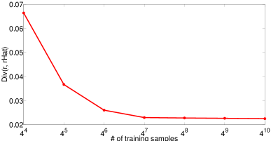
Figure 4: Density ratio estimate divergence $\mathbb{E}_{\mathsf{X}\sim P_{C}}\left[{D_{\varphi^{\dagger}}(r(\mathsf{X}),\hat{r}(\mathsf{X}))}\right]$ as a function of # of training samples.

H.2 Adaptive filtering experiments

Tables 8 – 13 present in extenso the experiments of $p$-LMS vs DN-$p$-LMS, as a function of $(p,q)$, whether target $\bm{u}$ is sparse or not, and the misestimation factor $\rho$ for $X_{p}$. We refer to Kivinen et al. [2006] for the formal definitions used for sparse / dense targets as well as for the experimental setting, which we have reproduced with the sole difference that the signal changes periodically each 1 000 iterations.

$\rho=0.1$	$\rho=0.2$	$\rho=0.3$	$\rho=0.4$	$\rho=0.5$	$\rho=0.6$
$\rho=0.7$	$\rho=0.8$	$\rho=0.9$	$\rho=\mbox{{1.0}}$	$\rho=1.1$	$\rho=1.2$
$\rho=1.3$	$\rho=1.4$	$\rho=1.5$	$\rho=1.6$	$\rho=1.7$

Table 8: Error($p$-LMS) - Error(DN-$p$-LMS) as a function of $t$ ($\in\{1,2,...,50000\}$), $\bm{u}$ = dense, $(p,q)=(1.17,6.9)$.

$\rho=0.1$	$\rho=0.2$	$\rho=0.3$	$\rho=0.4$	$\rho=0.5$	$\rho=0.6$
$\rho=0.7$	$\rho=0.8$	$\rho=0.9$	$\rho=\mbox{{1.0}}$	$\rho=1.1$	$\rho=1.2$
$\rho=1.3$	$\rho=1.4$	$\rho=1.5$	$\rho=1.6$	$\rho=1.7$

Table 9: Error($p$-LMS) - Error(DN-$p$-LMS) as a function of $t$ ($\in\{1,2,...,50000\}$), $\bm{u}$ = sparse, $(p,q)=(1.17,6.9)$.

$\rho=0.1$	$\rho=0.2$	$\rho=0.3$	$\rho=0.4$	$\rho=0.5$	$\rho=0.6$
$\rho=0.7$	$\rho=0.8$	$\rho=0.9$	$\rho=\mbox{{1.0}}$	$\rho=1.1$	$\rho=1.2$
$\rho=1.3$	$\rho=1.4$	$\rho=1.5$	$\rho=1.6$	$\rho=1.7$

Table 10: Error($p$-LMS) - Error(DN-$p$-LMS) as a function of $t$ ($\in\{1,2,...,50000\}$), $\bm{u}$ = dense, $(p,q)=(2.0,2.0)$.

$\rho=0.1$	$\rho=0.2$	$\rho=0.3$	$\rho=0.4$	$\rho=0.5$	$\rho=0.6$
$\rho=0.7$	$\rho=0.8$	$\rho=0.9$	$\rho=\mbox{{1.0}}$	$\rho=1.1$	$\rho=1.2$
$\rho=1.3$	$\rho=1.4$	$\rho=1.5$	$\rho=1.6$	$\rho=1.7$

Table 11: Error($p$-LMS) - Error(DN-$p$-LMS) as a function of $t$ ($\in\{1,2,...,50000\}$), $\bm{u}$ = sparse, $(p,q)=(2.0,2.0)$.

$\rho=0.1$	$\rho=0.2$	$\rho=0.3$	$\rho=0.4$	$\rho=0.5$	$\rho=0.6$
$\rho=0.7$	$\rho=0.8$	$\rho=0.9$	$\rho=\mbox{{1.0}}$	$\rho=1.1$	$\rho=1.2$
$\rho=1.3$	$\rho=1.4$	$\rho=1.5$	$\rho=1.6$	$\rho=1.7$

Table 12: Error($p$-LMS) - Error(DN-$p$-LMS) as a function of $t$ ($\in\{1,2,...,50000\}$), $\bm{u}$ = dense, $(p,q)=(6.9,1.17)$.

$\rho=0.1$	$\rho=0.2$	$\rho=0.3$	$\rho=0.4$	$\rho=0.5$	$\rho=0.6$
$\rho=0.7$	$\rho=0.8$	$\rho=0.9$	$\rho=\mbox{{1.0}}$	$\rho=1.1$	$\rho=1.2$
$\rho=1.3$	$\rho=1.4$	$\rho=1.5$	$\rho=1.6$	$\rho=1.7$

Table 13: Error($p$-LMS) - Error(DN-$p$-LMS) as a function of $t$ ($\in\{1,2,...,50000\}$), $\bm{u}$ = sparse, $(p,q)=(6.9,1.17)$.

Appendix I Comment: Theorem 1 is a scaled isometry in disguise (sometimes)

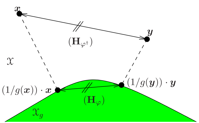
Figure 5: A depiction of the adaptive isometry that Theorem 1 provides.

Theorem 1 states in fact an isometry under some conditions, but an adaptive one in the sense that metrics involved rely on all parameters, and in particular on the points involved in the divergences (See Figure 5). Indeed, a simple Taylor expansion of the equation (2) (main file) shows that any such Bregman distortion with a twice differentiable generator can be expressed as:

$$D_{\varphi}(\bm{x}\|\bm{y}) = \frac{1}{2}\cdot(\bm{x}-\bm{y})^{\top}\textbf{H}_{\varphi}(\bm{x}-\bm{y})\>\>,$$ (141)

for some value of the Hessian $\textbf{H}_{\varphi}$ depending on $\bm{x},\bm{y}$ (see for example [Kivinen et al., 2006, Appendix I], [Amari and Nagaoka, 2000]). Hence, under the constraint that both $\varphi$ and $\varphi^{\dagger}$ are twice differentiable, eq. (3) becomes

$$g(\bm{x})\cdot\left(\frac{1}{g(\bm{x})}\cdot\bm{x}-\frac{1}{g(\bm{y})}\cdot\bm{y}\right)^{\top}\textbf{H}_{\varphi}\left(\frac{1}{g(\bm{x})}\cdot\bm{x}-\frac{1}{g(\bm{y})}\cdot\bm{y}\right) = (\bm{x}-\bm{y})^{\top}\textbf{H}_{\varphi^{\dagger}}(\bm{x}-\bm{y})\>\>.$$ (142)

Assuming $g$ non-negative (which, by the way, enforces the convexity of $\varphi^{\dagger}$), we get by taking square roots,

$$\sqrt{g(\bm{x})}\cdot\left\|\frac{1}{g(\bm{x})}\cdot\bm{x}-\frac{1}{g(\bm{y})}\cdot\bm{y}\right\|_{\textbf{H}_{\varphi}} = \left\|\bm{x}-\bm{y}\right\|_{\textbf{H}_{\varphi^{\dagger}}}\>\>,$$ (143)

which is a scaled isometry relationship between $\mathcal{X}_{g}$ (left) and $\mathcal{X}$ (right), but again the metrics involved depend on the arguments. Nevertheless, eq. (143) displays a sophisticated relationship between distances in $\mathcal{X}_{g}$ and in $\mathcal{X}$ which may prove useful in itself.

References

- Acharyya et al. [2013] S. Acharyya, A. Banerjee, and D. Boley. Bregman divergences and triangle inequality. In SDM, 2013.
- Amari and Nagaoka [2000] S.-I. Amari and H. Nagaoka. Methods of Information Geometry. Oxford University Press, 2000.
- Arthur and Vassilvitskii [2007] D. Arthur and S. Vassilvitskii. -means++ : the advantages of careful seeding. In 19 SODA, 2007.
- Banerjee et al. [2005] A. Banerjee, S. Merugu, I. Dhillon, and J. Ghosh. Clustering with Bregman divergences. JMLR, 6:1705–1749, 2005.
- Beck and Teboulle [2003] A. Beck and M. Teboulle. Mirror descent and nonlinear projected subgradient methods for convex optimization. Operations Research Letters, 31(3):167–175, 2003.
- Boissonnat et al. [2010] J.-D. Boissonnat, F. Nielsen, and R. Nock. Bregman Voronoi diagrams. DCG, 44(2):281–307, 2010.
- Boyd and Vandenberghe [2004] S. Boyd and L. Vandenberghe. Convex Optimization. Cambridge University Press, 2004. ISBN 0521833787.
- Buja et al. [2005] A. Buja, W. Stuetzle, and Y. Shen. Loss functions for binary class probability estimation and classification: Structure and applications, 2005. Unpublished manuscript.
- Buss and Fillmore [2001] S.-R. Buss and J.-P. Fillmore. Spherical averages and applications to spherical splines and interpolation. ACM Transactions on Graphics, 20:95–126, 2001.
- Cayton [2009] L. Cayton. Efficient bregman range search. In NIPS*22, pages 243–251, 2009.
- Cesa-Bianchi and Lugosi [2006] N. Cesa-Bianchi and G. Lugosi. Prediction, Learning and Games. Cambridge University Press, 2006.
- Collins et al. [2002] M. Collins, R. Schapire, and Y. Singer. Logistic regression, AdaBoost and Bregman distances. MLJ, 2002.
- Dhillon and Modha [2001] I. Dhillon and D.-S. Modha. Concept decompositions for large sparse text data using clustering. MLJ, 42:143–175, 2001.
- Dhillon and Tropp [2008] I.-S. Dhillon and J.-A. Tropp. Matrix nearness problems with Bregman divergences. SIAM Journal on Matrix Analysis and Applications, 29(4):1120–1146, 2008.
- Duchi et al. [2008] J. Duchi, S. Shalev-Shwartz, Y. Singer, and T. Chandra. Efficient projections onto the -ball for learning in high dimensions. In ICML ’08, pages 272–279, New York, NY, USA, 2008. ACM. ISBN 978-1-60558-205-4.
- Endo and Miyamoto [2015] Y. Endo and S. Miyamoto. Spherical k-means++ clustering. In Proc. of the 12th MDAI, pages 103–114, 2015.
- Galperin [1993] G.-A. Galperin. A concept of the mass center of a system of material points in the constant curvature spaces. Communications in Mathematical Physics, 154:63–84, 1993.
- Hazan and Kale [2012] E. Hazan and S. Kale. Projection-free online learning. In John Langford and Joelle Pineau, editors, ICML ’12, pages 521–528, New York, NY, USA, 2012. ACM.
- Hernández-Lobato et al. [2016] M. Hernández-Lobato, Y. Li, M. Rowland, D. Hernández-Lobato, T. Bui, and R.-E. Turner. Black-box alpha-divergence minimization. In 33rd ICML, 2016.
- Jaggi [2013] M. Jaggi. Revisiting Frank-Wolfe: Projection-free sparse convex optimization. In 30th ICML, 2013.
- Kivinen et al. [2006] J. Kivinen, M. Warmuth, and B. Hassibi. The -norm generalization of the LMS algorithm for adaptive filtering. IEEE Trans. SP, 54:1782–1793, 2006.
- Kuang et al. [2014] D. Kuang, S. Yun, and H. Park. SymNMF: nonnegative low-rank approximation of a similarity matrix for graph clustering. J. Global Optimization, 62:545–574, 2014.
- Kulis et al. [2009] B. Kulis, M.-A. Sustik, and I.-S. Dhillon. Low-rank kernel learning with Bregman matrix divergences. JMLR, 10:341–376, 2009.
- Menon and Ong [2016] A.-K. Menon and C.-S. Ong. Linking losses for class-probability and density ratio estimation. In ICML, 2016.
- Nock and Nielsen [2005] R. Nock and F. Nielsen. Fitting the Smallest Enclosing Bregman Ball. In Proc. of the 16 European Conference on Machine Learning, pages 649–656. Springer-Verlag, 2005.
- Nock and Nielsen [2009] R. Nock and F. Nielsen. Bregman divergences and surrogates for learning. IEEE PAMI, 31:2048–2059, 2009.
- Nock et al. [2008] R. Nock, P. Luosto, and J. Kivinen. Mixed Bregman clustering with approximation guarantees. In ECML, 2008.
- Nock et al. [2016] R. Nock, F. Nielsen, and S.-I. Amari. On conformal divergences and their population minimizers. IEEE Trans. IT, 62:527–538, 2016.
- Reid and Williamson [2011] M. Reid and R. Williamson. Information, divergence and risk for binary experiments. JMLR, 12:731–817, 2011.
- Reid and Williamson [2010] M.-D. Reid and R.-C. Williamson. Composite binary losses. JMLR, 11:2387–2422, 2010.
- Reisinger et al. [2010] J. Reisinger, A. Waters, B. Silverthorn, and R.-J. Mooney. Spherical topic models. In 27th ICML, pages 903–910, 2010.
- Rong et al. [2010] G. Rong, M. Jin, and X. Guo. Hyperbolic centroidal Voronoi tessellation. In 14 ACM SPM, 2010.
- Schwander and Nielsen [2013] O. Schwander and F. Nielsen. Matrix Information Geometry, chapter Learning Mixtures by Simplifying Kernel Density Estimators, pages 403–426. Springer Berlin Heidelberg, 2013.
- Shahani et al. [2015] A.-J. Shahani, E.-B. Gulsoy, V.-J. Roussochatzakis, J.-W. Gibbs, J.-L. Fife, and P.-W. Voorhees. The dynamics of coarsening in highly anisotropic systems: Si particles in AlSi liquids. Acta Materialia, 97:325 – 337, 2015.
- Shalev-Shwartz et al. [2007] S. Shalev-Shwartz, Y. Singer, and N. Srebro. Pegasos: Primal estimated sub-gradient solver for SVM. In ICML ’08, page 807–814. ACM, 2007. ISBN 978-1-59593-793-3.
- Shimodaira [2000] H. Shimodaira. Improving predictive inference under covariate shift by weighting the log-likelihood function. Journal of Statistical Planning and Inference, 90(2):227 – 244, 2000. ISSN 0378-3758.
- Straub et al. [2014] J. Straub, G. Rosman, O. Freifeld, J.-J. Leonard, and J.-W. Fisher III. A mixture of Manhattan frames: Beyond the Manhattan world. In Proc. of the 27th IEEE CVPR, pages 3770–3777, 2014.
- Straub et al. [2015a] J. Straub, N. Bhandari, J.-J. Leonard, and J.-W. Fisher III. Real-time Manhattan world rotation estimation in 3d. In Proc. of the 27th IROS, pages 1913–1920, 2015a.
- Straub et al. [2015b] J. Straub, T. Campbell, J.-P. How, and J.-W. Fisher III. Small-variance nonparametric clustering on the hypersphere. In Proc. of the 28th IEEE CVPR, pages 334–342, 2015b.
- Straub et al. [2015c] J. Straub, J. Chang, O. Freifeld, and J.-W. Fisher III. A Dirichlet process mixture model for spherical data. In Proc. of the 18th AISTATS, 2015c.
- Sugiyama et al. [2012] M. Sugiyama, T. Suzuki, and T. Kanamori. Density-ratio matching under the Bregman divergence: a unified framework of density-ratio estimation. AISM, 64(5):1009–1044, 2012. ISSN 0020-3157.
- Ungar [2014] A.-A. Ungar. Mathematics Without Boundaries: Surveys in Interdisciplinary Research, chapter An Introduction to Hyperbolic Barycentric Coordinates and their Applications, pages 577–648. Springer New York, 2014.
- Vidal [2011] R. Vidal. Subspace clustering. IEEE Signal Processing Magazine, 28:52–68, 2011.
- Williamson et al. [2014] R.-C. Williamson, E. Vernet, and M.-D. Reid. Composite multiclass losses, 2014. Unpublished manuscript.
- Zhang and Sra [2016] H. Zhang and S. Sra. First-order methods for geodesically convex optimization. CoRR, abs/1602.06053, 2016.