Casimir energies of self-similar plate configurations
Abstract
We construct various self-similar configurations using parallel -function plates and show that it is possible to evaluate the Casimir interaction energy of these configurations using the idea of self-similarity alone. We restrict our analysis to interactions mediated by a scalar field, but the extension to the electromagnetic field is immediate. Our work unveils an easy and powerful method that can be easily employed to calculate the Casimir energies of a class of self-similar configurations. As a highlight, in an example, we determine the Casimir interaction energy of a stack of parallel plates constructed by positioning -function plates at the points constituting the Cantor set, a prototype of a fractal. This, to our knowledge, is the first time that the Casimir energy of a fractal configuration has been reported. Remarkably, the Casimir energy of some of the configurations we consider turn out to be positive, and a few even have zero Casimir energy. For the case of positive Casimir energy that is monotonically decreasing as the stacking parameter increases the interpretation is that the pressure of vacuum tends to inflate the infinite stack of plates. We further support our results, derived using the idea of self-similarity alone, by rederiving them using the Green’s function formalism. These expositions gives us insight into the connections between the regularization methods used in quantum field theories and regularized sums of divergent series in number theory.
I Introduction
Physical phenomena associated with the interaction energy between two bodies, arising as a direct manifestation of the quantum fluctuations in the field mediating the interactions, is broadly termed the Casimir energy. The Casimir force between two parallel conducting plates associated with this interaction energy was first theoretically predicted by Casimir in Ref. Casimir (1948). In this article, for simplicity in the mathematical analysis, we consider the interactions to be mediated by a scalar field. Nonetheless, many of the physical interpretations and intuition we have amassed for the electromagnetic field can often be extended to the scalar model, especially for the case of perfect conductors because one of the modes for the electromagnetic case can be represented by a scalar field satisfying Dirichlet boundary conditions. Since the original calculation by Casimir, the Casimir energies of special geometries like parallelepipeds Lukosz (1971); Ambjørn and Wolfram (1983a, b), spheres Boyer (1968); Milton et al. (1978), and cylinders DeRaad and Milton (1981); Cavero-Pelaez and Milton (2005) has been reported both for the scalar field and for the electromagnetic field. More recently, using the multiple scattering formulation Balian and Duplantier (1977, 1978) the single-body contributions were generically separated from the total energy Kenneth and Klich (2006); Emig et al. (2008); Milton and Wagner (2008), and it has become possible to compute Casimir energies for arbitrary shaped disjoint objects. An extension of the theory so as to include dynamical Casimir effects leads to fundamental quantum mechanical phenomena such as Casimir friction, c.f., for instance, the recent review of Ref. Milton et al. (2016).
A generalization of these ideas to more than two bodies was given in Refs. Schaden (2011); Shajesh and Schaden (2011, 2012), but explicit solutions for the Green’s functions were reported only for configurations with three bodies. Here, in Sec. III, we find solutions to the Green’s function for four bodies, and then, we go further and express the solution to the Green’s function for bodies as a recursion relation in terms of the Green’s functions for bodies. This procedure then lets us extend our solutions for the Green’s functions for an infinite sequence of objects by taking the limit .
In Sec. IV, we use the solution for the Green’s function for an infinite sequence of objects to calculate the Casimir energy of self-similar configurations. In particular, we calculate the Casimir energy of parallel -function plates satisfying Dirichlet boundary conditions that are positioned in various patterns to construct simple self-similar configurations. The Casimir energy of these infinite sequence of plates comes to be positive, negative, or zero, suggesting that the pressure of vacuum tends to inflate, deflate, or balance the infinite stack of plates. These results are obtained by regularizing sums for divergent series, which on its own might not be convincing. But, the highlight of this article, is that we are able to derive all of the above results using the idea of self-similarity alone in a self-contained manner. We begin our discussion in Sec. II by presenting these derivations using the idea of self-similarity, which we again point out are completely independent of the derivation using Green’s function formalism that we apply later in Secs. III and IV to further support our claims. In Sec. V, we present an analogy between our present study and the theory of the piecewise uniform string. In Sec. VI, we present few concluding remarks and an outlook.
II Casimir interaction energies for self-similar configurations
A self-similar set contains the set itself as a subset, or more generally, there exists a one-to-one mapping between the elements of the set and a subset of the set. The property of self-similarity is illustrated well when it is used to sum a series. Consider an infinite sum
| (1) |
Using the idea of self-similarity we can identify the following relation for the sum,
| (2) |
which immediately leads to the conclusion that the sum of the series is . We can extend this idea of self-similarity to ‘sum’ a divergent series too. For example, for the divergent sum
| (3) |
using the idea of self-similarity, we can identify the relation
| (4) |
which assigns the value to the above divergent sum and is interpreted as the ‘sum’ of the divergent series. Even though values assigned to divergent series in this manner are now well accepted as a regularized sum, the perplexities associated with these manipulations in the spirit of Ref. Hardy (1956) still linger on. Here, we construct self-similar configurations of parallel plates, and using the idea of self-similarity along the lines of the illustrations above, we derive the Casimir interaction energies for these configurations.
We construct a planar configuration consisting of an infinite sequence of parallel -function plates. By -function plates we mean infinitely thin plates that are mathematically described by Dirac -functions. The position of the plates are given by the sequence
| (5) |
the ‘strength’ of the plates are given by the sequence
| (6) |
and their interactions are mediated through a scalar quantum field, with the plates described by the potentials
| (7) |
When the dynamics of the plates is neglected (valid when the masses of the plates are large), the vacuum to vacuum transitions induced by the quantum fluctuations of the scalar field leads to energy and momentum densities, which are given in terms of the energy-momentum tensor and the associated Green’s function for the scalar field. The total energy, obtained by integrating the energy density over all space, is termed the vacuum energy or the Casimir energy or the zero point energy. Here, we discuss the Casimir energy of an infinite sequence of parallel -function plates.
It is well known, for example, see Ref. Balian and Duplantier (1977, 1978); Ravndal (2000); Bulgac and Wirzba (2001); Bulgac et al. (2006); Kenneth and Klich (2006); Shajesh and Schaden (2011), that the total energy per unit area, , for two parallel plates separated by distance , can be decomposed in terms of the respective one-body energies as
| (8) |
where is the energy of the vacuum in the absence of the two objects, , , are the one-body energies associated to the individual objects, and is the interaction energy per unit area of the plates. In general, the one-body energies and the bulk energy diverge, and the Casimir interaction energy per unit area is finite and is distinctly isolated by its dependence on the distance , a signature of the interaction between the two plates. The Casimir interaction energy between two plates, mediated through a scalar field satisfying Dirichlet boundary conditions on the plates is given by, for example see Refs. Elizalde and Romeo (1991); Milton (2001),
| (9) |
which is exactly half of the Casimir interaction energy for two perfectly conducting plates mediated through electromagnetic fields. We are primarily interested in the interaction energy term in Eq. (8), which for multi-object configurations will get many-body contributions. We do not bother to separate this interaction energy into two-body, three-body, etc., like in Ref. Shajesh and Schaden (2011), and evaluate the total Casimir interaction energy. After all the one-body contributions has been subtracted, in addition to the bulk energy , the remaining Casimir interaction energy is in general finite, unless any two plates come into contact.
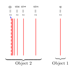
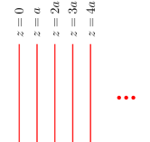
Let us consider an infinite sequence of plates placed at the following positions:
| (10) |
see FIG. 1, such that the distances between the plates successively decrease by a factor of two. Let us analyze the energy break up of this infinite sequence of plates by interpreting the single plate at as Object 1 and the rest of the plates to constitute Object 2. Using the decomposition of energy in Eq. (8), we can write
| (11) |
where we have isolated the single-body contributions to the energy explicitly. The single-body contributions, in this manner, cancel out in Eq. (11) to give
| (12) |
which requires some elaboration because we have used the idea of self-similarity in writing Eq. (12). The interaction energy of the complete stack of plates in FIG. 1 is on the left of Eq. (12). The first term on the right of Eq. (12) is the interaction energy of the plates constituting Object 2 in FIG. 1. And, the second term on the right of Eq. (12) is the interaction energy between Object 2 and Object 1. The idea of self-similarity has been used to note that the energy of Object 2 is equal to the energy of the complete stack evaluated for a rescaled parameter, here . The interaction energy is a function of alone (for Dirichlet plates) because that is the only parameter in the problem, and on dimensional grounds, we can argue that
| (13) |
Using the scaling argument of Eq. (13) in Eq. (12), we identify the relation involving the Casimir interaction energy of the infinite sequence of plates in FIG. 1,
| (14) |
which is the analog of the relation for infinite series in Eq. (2), here for the Casimir interaction energies.
The relation in Eq. (14) allows us to evaluate in terms of the interaction energy between Object 1 and Object 2 given by . In general it is a difficult task to evaluate the interaction energy . But, if each of the individual plates in the stack satisfy Dirichlet boundary conditions, which are called Dirichlet plates, there is considerable simplicity in the analysis because a Dirichlet plate physically disconnects the two spaces across it. For example, explicit decomposition of the total energy in terms of single-body, two-body, and three-body energies, and how they conspire such that the Casimir interaction energy is given completely in terms of interaction of two Dirichlet plates was described in detail in Ref. Shajesh and Schaden (2011). As a consequence, each Dirichlet plate can only interact with its closest neighbor on the left and on the right. Thus, the interaction energy between the two bodies in FIG. 1 is given by the Casimir interaction energy of two Dirichlet plates of Eq. (9), separated in this case by distance , which is the distance between the plates at and in FIG. 1. Thus, we have
| (15) |
which immediately leads to the Casimir interaction energy per unit area for the complete stack in FIG. 1 given by
| (16) |
Thus, using the idea of self-similarity, in a self-contained derivation, we have derived the Casimir interaction energy of an infinite stack of plates. Remarkably, the sign of the Casimir interaction energy for this configuration is positive. Thus, the tendency for the infinite sequence of plates in FIG. 1 is to inflate due to the pressure of vacuum.
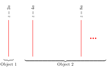
We consider another example to point out that the Casimir interaction energy is not always positive for an infinite sequence of plates. We consider an infinite sequence of plates placed at the following positions:
| (17) |
as described in FIG. 2. (We start from because it extends the series in Eq. (10) and later allows us to merge the two stacks.) Using the idea of self-similarity, we identify the relation
| (18) |
Then, using
| (19) |
we immediately learn that
| (20) |
This suggests that the tendency of the stack of plates in FIG. 2 is to contract under the pressure of vacuum.
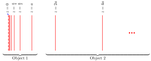
Having derived the Casimir interaction energy of two independent stacks, we now place them such that they can be imagined to be a sequence that extends on both ends, given by
| (21) |
as described in FIG. 3. Since we already derived the energies for the individual stacks, we can calculate the energy of the complete stack using the two-body break up of the Casimir energies. Thus, we have the total interaction energy of the two stacks given by the relation
| (22) |
where the first term on the right is the Casimir interaction energy of the first stack given by Eq. (16), the second term is the Casimir interaction energy of the second stack given by Eq. (20), and the third term is the interaction energy of the two stacks given by the energy of two Dirichlet plates in Eq. (9). Together we have
| (23) |
which suggests that the Casimir energy of the two stacks, in conjunction, in FIG. 3, is exactly zero. Apparently, the pressure due to vacuum that tends to inflate the first stack, when in isolation, and contract the second stack in isolation, when in conjunction, conspire to balance these opposite tendencies exactly. It can be easily verified that this cancellation is independent of the particular choice of breakup into Objects 1 and 2, which is a signature of self-similarity.
In our last example, we highlight a self-similar configuration of plates motivated from the Cantor set. We place a -function plate at every point of the Cantor set. The classic Cantor set is obtained by iteratively dividing a line segment into three parts and deleting the central region each time. We build our stack of plates by placing a -function plate at the edge of the remaining segments in each iteration, see FIG. 4. The idea of self-similarity and the two-body break up of energy then leads to the relation, in the Dirichlet limit,
| (24) |
Then, using
| (25) |
we have the Casimir interaction for the configuration in FIG. 4 given by
| (26) |
The positive sign signifies that the pressure due to vacuum tends to inflate the stack in FIG. 4.
In the following section, we further support the above derivations for the Casimir interaction energies for self-similar plates by evaluating the explicit Green’s functions for these configurations. We find the Green’s function for parallel -function plates given in terms of the corresponding combinations of parallel -function plates. We are interested in the limit of infinite plates obtained by taking the limit .
III Green’s function for parallel -function plates
The Green’s function for parallel -function plates satisfies the equation
| (27) |
The translation symmetry in the plane of plates and static considerations allows the corresponding modes to be bunched as . We also make Euclidean rotation and replace . The free Green’s function, corresponding to the absence of all the plates, satisfies the equation
| (28) |
and has the solution
| (29) |
We use the ansatz
| (30) |
which is motivated from the discussions in Ref. Shajesh and Schaden (2011). In Eq. (30), we have used matrix notation and summation convention to symbolically write
| (31) |
where the components of the vector are free Green’s functions when one of the source points is on the -th plate, that is,
| (32) |
The components of the dyadic are independent of and and are given by the matrix equation, see the Appendix A,
| (33) |
where is the identity matrix,
| (34) |
is a diagonal matrix of coupling constants, and
| (35) |
is a matrix whose components are free Green’s functions evaluated from the -th to the -th plate. That is,
| (36) |
For convenience, we introduce dimensionless quantities
| (37) |
The matrix equations of Eq. (33) are the Faddeev equations Faddeev (1965); Merkuriev and Faddeev (1993) that were introduced in the study of nuclear many-body scattering.
For a single plate, , we immediately have
| (38) |
The corresponding Green’s function, given by Eq. (30) for , has the explicit form
| (39) |
The solution for the Green’s function in Eq. (39) is valid for all and , the difference in the behavior decided by the absolute values and . The compactness in the solution for planar geometry is a direct consequence of this feature, which does not extend to other geometries.
For two plates, , we solve Eq. (33) and find
| (40) |
where
| (41) |
The corresponding Green’s function, given by Eq. (30) for , has the explicit form
| (46) |
where we used the property of trace to write the second term in Eq. (30) in the form
| (47) |
For three plates, , we solve Eq. (33) and find
| (48) |
where the determinant can be written in the form
| (49) |
Here, we have introduced the generalized form of the notation in Eq. (36),
| (50) |
the right side of which are given in terms of 1-plate Green’s functions of Eq. (39). The corresponding Green’s function is given by Eq. (30) for , the second term of which has the explicit form
| (57) |
For , we solve Eq. (33) and find
| (58) |
where
| (59) |
the right side of which are given in terms of 2-plate Green’s functions of Eq. (46). The determinant
| (60) |
III.1 Recursion relation
From the pattern that emerges for the above cases, we can write down the the Green’s function for -function plates as
| (61) |
This can then be immediately extended for the case. The Green’s function for plates is given in terms of all possible Green’s function for plates, obtained by deleting two plates. In this sense, we have a recursion relation for the Green’s function. The Green’s function presented as a recursion relation is very suitable for the kind of problems we are addressing here. Our method for finding the Green’s function for bodies is fundamentally different from the earlier techniques used to find the Green’s function for multilayered systems, for example, see Refs. Reed et al. (1987); Tomaš (1995); Zhou and Spruch (1995).
III.2 Green’s function for a sequence of Dirichlet plates
Let us consider the very special case of every -function plate being a Dirichlet plate. This is described by the limiting conditions,
| (62) |
for all ’s. We go back to the matrix equation in Eq. (33) and find that in the Dirichlet limit (in all plates) we have
| (63) |
where was defined in Eq. (35) and is a matrix built out of all possible free Green’s functions. The inverse of is immediately evaluated to yield the transition matrix as a tridiagonal matrix,
| (64) |
where
| (65) |
and
| (66) |
and
| (67) |
such that is the magnitude of the distance between the -th and -th parallel plate. The Green’s function is then completely determined by the transition matrix using Eq. (30).
IV Casimir energy for parallel -function plates
.
The Casimir energy per unit area for parallel -function plates is determined in terms of the Green’s function Shajesh and Schaden (2011),
| (68) |
Using the ansatz of Eq. (30) in Eq. (68), we have
| (69) |
where is the energy in the absence of all plates, a divergent quantity, often called the bulk free energy, given by
| (70) |
Observing that , one notes that this divergent contribution is proportional to the volume and independent of any of the physical parameters of the problem. For planar geometries that we are discussing the -integral in Eq. (69) can be evaluated to yield
| (71) |
where
| (72) |
where is the distance between the -th and -th parallel plate, defined previously. Thus, we have the Casimir energy per unit area given by
| (73) |
Other than the bulk free energy term, , we also have divergent single-body contributions from each of the individual plates. The Casimir energy of a single plate, say plate 1, in the absence of all other plates, is given using Eq. (73) as
| (74) |
which is divergent and independent of any of the physical parameters of the problem. The second term in Eq. (73) has divergent contributions of these, and we study the contribution to the energy after these single-body contributions, in addition to the bulk free energy, has been subtracted. To this end we define the Casimir interaction energy per unit area, because they involve interactions between the plates, in the spirit of Eq. (8),
| (75) |
which is free of divergences unless any of the individual plates touch.
IV.1 Finite sequence of Dirichlet plates
For a sequence of Dirichlet plates the Casimir energy is given by
| (76) |
where the contribution of inside the square brackets comes from summing the ’s in the diagonal terms of the transition matrix in Eq. (64). This term and the first two terms inside the sum in Eq. (76) can be combined as
| (77) |
which is identified as the sum of single-body (divergent) contributions to the Casimir energy from the individual plates, see Eq. (74). Thus, the Casimir interaction energy per unit area, introduced in Eq. (75), for parallel Dirichlet plates is given by the expression
| (78) |
which using the integral
| (79) |
is expressed as
| (80) |
This result is not surprising because a Dirichlet plate physically disconnects the two half-spaces across it.
IV.2 Infinite sequence of Dirichlet plates
In the example of FIG. 1 given by the sequence of plates in Eq. (10) we have
| (81) |
which together with Eq. (80) leads to the Casimir interaction energy for this configuration given by the expression
| (82) |
Using the idea of self-similarity in the context of series we identify the relation , with . Thus, we make the formal assignment
| (83) |
to determine the the Casimir interaction energy for this configuration to be
| (84) |
exactly as we derived earlier in Eq. (16).
Next, we consider an infinite sequence of Dirichlet plates given using Eq.(17), as described in FIG. 2, such that
| (85) |
We have the Casimir interaction energy for this configuration, using Eq. (80), given by the expression
| (86) |
This involves the convergent series
| (87) |
which implies that the Casimir interaction energy for this configuration is
| (88) |
exactly as we derived earlier in Eq. (20).
As the final example, we consider equidistant Dirichlet plates filling half of the space, that is,
| (89) |
such that
| (90) |
for all , see FIG. 5. We have the Casimir interaction energy for this configuration given by the expression
| (91) |
If we now make the formal assignment
| (92) |
the Casimir interaction energy of this infinite equidistant Dirichlet plates filling half of the space changes sign,
| (93) |
That is, again, the tendency for the plates is to inflate under the pressure of vacuum.
V Analogy to the theory of the piecewise uniform string
There exists an interesting analogy between the theory considered in this paper and Casimir theory of the piecewise uniform string. To our knowledge, this analogy has not been pointed out before. Let us start by outlining some basic aspects of this kind of string theory, assuming first that the system is a material ring of total length divided into two pieces, . The system exhibits small oscillations with amplitude , where is the position coordinate and the time (the usual convention in string theory). The string tensions are and , and the mass densities are and , adjusted such that the speed of sound is everywhere the same as the speed of light,
| (94) |
In this sense, the string model is relativistic. At the two junctions, the displacement , as well as the transverse force , are continuous. The equation of motion
| (95) |
is solved for the right-and left-moving modes. The dispersion relation determining the eigenfrequencies is
| (96) |
where is the tension ratio.
The Casimir energy, given by the difference between the total energy and the energy for a uniform string, is
| (97) |
It can be regularized in at least three different ways:
-
•
Use of a cutoff factor , , being applied to the energy expression before summing over the modes.
-
•
Use of the contour integration method, which means applying the so-called argument principle
(98) which holds for any meromorphic function , where and denote the zeros and the poles, respectively. In our case, is essentially the left-hand side of the expression in Eq. (96) above.
-
•
Use of the zeta-function method, which in our case means applying the analytic continuation of the Hurwitz function defined as
(99)
All methods lead to the same answer for the Casimir energy, due to the relativistic property in Eq. (94). We give the expression only for the simple case when ,
| (100) |
The energy is seen to be zero (if ) or otherwise negative. The difference in the coefficient relative to Eq. (9) is because we are working in 1+1 spacetime dimensions here as compared to 3+1 spacetime dimensions earlier.
To our knowledge, this model was first suggested by Brevik and Nielsen in Brevik and Nielsen (1990), c.f. also Li et al. Li et al. (1991), applying the Hurwitz zeta function. The contour integration method was applied to this problem by Brevik and Elizalde Brevik and Elizalde (1994). Later on, there have been developments in various directions, including the generalization to a string composed of pieces, all of the same length Brevik and Nielsen (1995). General reviews, containing more references, can be found in Refs. Brevik et al. (2001); Berntsen et al. (1997); Elizalde (1995). A generalization to the case of a nonrelativistic string, (the velocity of sound being different in the different pieces,) has been given in Ref. Hadasz et al. (2000).
We are now in a position to see the natural relationship to the model with self-similar plates. Consider the case where the positions are given by . The difference between the positions of the first and last plate in the limit where the number of plates is infinity is finite, equal to . Assume now that the composite string is divided into alternating type 1 and type 2 sections, spaced according to the same prescription. This means simply that the string length is to be identified with . It would be of interest to carry out a calculation of the Casimir energy for this special kind of string. We do not enter into this task here, however, but limit ourselves to pointing out the analogy.
The relativistic property of the system will still be maintained, due to Eq. (94), although an evident physical restriction is that the dielectric property cannot be maintained of the elements when their lengths go towards zero. The limit of infinitely many pieces is an idealized model.
VI Conclusions and outlook
We have derived the Casimir energies of simple self-similar configurations consisting of parallel -function plates satisfying Dirichlet boundary conditions using the idea of self-similarity alone. Then, we have corroborated our results for Casimir energies using the completely independent Green’s functions formalism. We have thus shown that an infinite stack of parallel plates can have positive, negative, or zero Casimir energy. In particular, we have successfully derived the Casimir energy of a stack of plates positioned at the points of the Cantor set, thus computing the Casimir energy of a simple fractal for the first time.
A fractal often has unusual scaling behavior, which often leads to noninteger fractal dimensions for volume, area, or perimeter for these geometric shapes. The Casimir energy also depends on the geometry of the cavity that binds the field. In this context, the connections between the Casimir energy and the Weyl’s problem on the asymptotic distribution of the eigenvalues for the wave equation for smooth boundaries is well documented, for example, see Refs. Baltes and Hilf (1974); Balian and Bloch (1970, 1971). Berry in Refs. Berry (1979, 1996) conjectured that the Weyl’s formula in Ref. Weyl (1911) for the asymptotic mode number extends for fractal regions and/or surfaces. This Berry-Weyl conjecture has been shown to hold, if the dimensions of the regions and surfaces are interpreted as the Minkowski-Bouligand dimension Lapidus and Fleckinger (1988) instead of the Hausdorff-Besicovitch dimension as originally proposed by Berry. The example consisting of parallel plates positioned at the points of a Cantor set has the dimension for its boundary equal to 2 because it is bounded by two-dimensional planes, and the volume dimension of the Cantor set is . The suggestion seems to be that it might be possible to read out the fractal dimension of a region from its Casimir energy Kigami and Lapidus (1993). In the example of the Cantor set, the total single-body energy is given by . For identical plates, is the same for all the plates. Thus, it factors out of the sum, and the remaining sum involves the addition of all the points of the Cantor set, which is suggestive evidence of the Weyl-Berry conjecture.
The only Casimir energy calculation that has been achieved for an infinite stack of plates before our work is probably that of equidistant parallel plates, in the spirit of our discussion in Sec. V. Using periodic boundary conditions, dictated by the periodicity of the plates, the problem reduces to finding the dispersion relation that determines the modes. Having described a formalism that could be used to work with configurations that does not involve equidistant plates, one could now entertain the idea of calculating the Casimir energy of a quasi-crystal. The remarks on the Poisson summation formula in the context of a quasi-crystal in Ref. Ninham and Lidin (1992) and on temperature inversion symmetry in the finite-temperature Casimir effect in Ref. Ravndal and Tollefsen (1989) might be indicative of this possibility.
*
Appendix A Proof of the Faddeev Equations (33)
Operating two derivatives with respect to in the ansatz of Eq. (30), we obtain
| (101) |
which using the differential equations for , , and , in Eqs. (27), (28), and (32), leads to the relation
| (102) |
Integrating Eq. (102) over from to for small , we have
| (103) |
in which there is no summation on . At this point, we note that these Green’s functions satisfy the reciprocity theorem
| (104) |
which requires the transition matrix to be symmetric,
| (105) |
We, of course, also have
| (106) |
We use the ansatz in Eq. (30) to replace the left-hand side of Eq. (103), operate it with two derivatives with respect to , and use the differential equation for in Eq. (28) in conjunction with the reciprocal symmetry of Green’s function to derive
| (107) |
Integrating Eq. (107) over from to for small , we have
| (108) |
which when rearranged, using Eq. (37), and expressed in vector notation is the Faddeev equation in Eq. (33).
Acknowledgements.
We dedicate this work to the memory of Martin Schaden, who passed away while this paper was being refereed. The ideas in the present paper emerged from Martin’s work in Refs.Schaden (2011); Shajesh and Schaden (2011), and we remember him for the collaborative assistance. K.V.S. would like to thank Jerzy Kocik and P. Sivakumar for discussions on the Apollonian gasket, which directly led to conducting this study. We thank Mathias Boström and Jose M. Muñoz-Castañeda for feedback on the manuscript and pointing us to relevant references. We acknowledge support from the Research Council of Norway (Project No. 250346). I.C.P. acknowledges support from Centro Universitario de la Defensa (Grant No. CUD2015-12), Spanish MINECO/FEDER (Grant No. FPA2015-65745-P), and DGA-FSE (Grant No. 2015-E24/2).References
- Casimir (1948) H. B. G. Casimir, “On the attraction between two perfectly conducting plates,” Kon. Ned. Akad. Wetensch. Proc. 51, 793 (1948).
- Lukosz (1971) W. Lukosz, “Electromagnetic zero-point energy and radiation pressure for a rectangular cavity,” Physica 56, 109 (1971).
- Ambjørn and Wolfram (1983a) J. Ambjørn and S. Wolfram, “Properties of the vacuum. 1. Mechanical and thermodynamic,” Ann. Phys. 147, 1 (1983a).
- Ambjørn and Wolfram (1983b) J. Ambjørn and S. Wolfram, “Properties of the vacuum. 2. Electrodynamic,” Ann. Phys. 147, 33 (1983b).
- Boyer (1968) T. H. Boyer, “Quantum electromagnetic zero-point energy of a conducting spherical shell and the Casimir model for a charged particle,” Phys. Rev. 174, 1764 (1968).
- Milton et al. (1978) K. A. Milton, L. L. DeRaad, Jr., and J. S. Schwinger, “Casimir selfstress on a perfectly conducting spherical shell,” Ann. Phys. 115, 388 (1978).
- DeRaad and Milton (1981) L. L. DeRaad, Jr. and K. A. Milton, “Casimir self-stress on a perfectly conducting cylindrical shell,” Ann. Phys. 136, 229 (1981).
- Cavero-Pelaez and Milton (2005) I. Cavero-Pelaez and K. A. Milton, “Casimir energy for a dielectric cylinder,” Ann. Phys. 320, 108 (2005).
- Balian and Duplantier (1977) R. Balian and B. Duplantier, “Electromagnetic waves near perfect conductors. I. Multiple scattering expansions. Distribution of modes,” Ann. Phys. 104, 300 (1977).
- Balian and Duplantier (1978) R. Balian and B. Duplantier, “Electromagnetic waves near perfect conductors. II. Casimir effect,” Ann. Phys. 112, 165 (1978).
- Kenneth and Klich (2006) O. Kenneth and I. Klich, “Opposites attract: A theorem about the Casimir force,” Phys. Rev. Lett. 97, 160401 (2006).
- Emig et al. (2008) T. Emig, N. Graham, R. L. Jaffe, and M. Kardar, “Casimir forces between compact objects. I. The scalar case,” Phys. Rev. D 77, 025005 (2008).
- Milton and Wagner (2008) K. A. Milton and J. Wagner, “Multiple scattering methods in Casimir calculations,” J. Phys. A 41, 155402 (2008).
- Milton et al. (2016) K. A. Milton, J. S. Høye, and I. Brevik, “The reality of Casimir friction,” Symmetry 8, 29 (2016).
- Schaden (2011) M. Schaden, “Irreducible many-body Casimir energies of intersecting objects,” Europhys. Lett. 94, 41001 (2011).
- Shajesh and Schaden (2011) K. V. Shajesh and M. Schaden, “Many-body contributions to Green’s functions and Casimir energies,” Phys. Rev. D 83, 125032 (2011).
- Shajesh and Schaden (2012) K. V. Shajesh and M. Schaden, “Significance of Many-Body Contributions to Casimir Energies,” Proceedings, 10th conference on quantum field theory under the influence of external conditions (QFEXT 11), Int. J. Mod. Phys. Conf. Ser. 14, 521 (2012).
- Hardy (1956) G. H. Hardy, Divergent series (Clarendon, Oxford, 1956).
- Ravndal (2000) F. Ravndal, “Problems with the Casimir vacuum energy,” in Problems with Vacuum Energy (Copenhagen, Denmark, 2000) arXiv:hep-ph/0009208 [hep-ph] .
- Bulgac and Wirzba (2001) A. Bulgac and A. Wirzba, “Casimir interaction among objects immersed in a fermionic environment,” Phys. Rev. Lett. 87, 120404 (2001).
- Bulgac et al. (2006) A. Bulgac, P. Magierski, and A. Wirzba, “Scalar Casimir effect between Dirichlet spheres or a plate and a sphere,” Phys. Rev. D 73, 025007 (2006).
- Elizalde and Romeo (1991) E. Elizalde and A. Romeo, “Essentials of the Casimir effect and its computation,” Am. J. Phys. 59, 711 (1991).
- Milton (2001) K. A. Milton, The Casimir effect: Physical manifestations of zero-point energy (World Scientific, Singapore, 2001).
- Faddeev (1965) L. D. Faddeev, Mathematical aspects of the three-body problem in the quantum scattering theory (Israel Program for Scientific Translations, Jerusalem, 1965).
- Merkuriev and Faddeev (1993) S. P. Merkuriev and L. D. Faddeev, Quantum scattering theory for several particle systems (Kluwer Academic, Dordrecht, The Netherlands, 1993).
- Reed et al. (1987) C. E. Reed, J. Giergiel, J. C. Hemminger, and S. Ushioda, “Dipole radiation in a multilayer geometry,” Phys. Rev. B 36, 4990 (1987).
- Tomaš (1995) M. S. Tomaš, “Green function for multilayers: Light scattering in planar cavities,” Phys. Rev. A 51, 2545 (1995).
- Zhou and Spruch (1995) F. Zhou and L. Spruch, “van der Waals and retardation (Casimir) interactions of an electron or an atom with multilayered walls,” Phys. Rev. A 52, 297 (1995).
- Brevik and Nielsen (1990) I. Brevik and H. B. Nielsen, “Casimir energy for a piecewise uniform string,” Phys. Rev. D 41, 1185 (1990).
- Li et al. (1991) X. Li, X. Shi, and J. Zhang, “Generalized Riemann -function regularization and Casimir energy for a piecewise uniform string,” Phys. Rev. D 44, 560 (1991).
- Brevik and Elizalde (1994) I. Brevik and E. Elizalde, “New aspects of the Casimir energy theory for a piecewise uniform string,” Phys. Rev. D 49, 5319 (1994).
- Brevik and Nielsen (1995) I. Brevik and H. B. Nielsen, “Casimir theory for the piecewise uniform string: Division into pieces,” Phys. Rev. D 51, 1869 (1995).
- Brevik et al. (2001) I. Brevik, A. A. Bytsenko, and B. M. Pimentel, “Thermodynamic properties of the relativistic composite string: Expository remarks,” in Theoretical Physics 2002: Part 2, edited by T. F. George and H. F. Arnoldus (Nova, New York, 2001) p. 117, arXiv:hep-th/0108116 [hep-th] .
- Berntsen et al. (1997) M. H. Berntsen, I. Brevik, and S. D. Odintsov, “Casimir theory for the piecewise uniform relativistic string,” Ann. Phys. 257, 84 (1997).
- Elizalde (1995) E. Elizalde, Ten physical applications of spectral zeta functions (Springer, Berlin, 1995) chapter 7.
- Hadasz et al. (2000) L. Hadasz, G. Lambiase, and V. V. Nesterenko, “Casimir energy of a nonuniform string,” Phys. Rev. D 62, 025011 (2000).
- Baltes and Hilf (1974) H.P. Baltes and E. R. Hilf, Spectra of finite systems, Tech. Rep. (BI-Wissenschaftsverlag, Bibliographisches Institut Mannheim, 1974).
- Balian and Bloch (1970) R. Balian and C. Bloch, “Distribution of eigenfrequencies for the wave equation in a finite domain,” Ann. Phys. 60, 401 (1970).
- Balian and Bloch (1971) R. Balian and C. Bloch, “Distribution of eigenfrequencies for the wave equation in a finite domain. II. Electromagnetic field. Riemannian spaces,” Ann. Phys. 64, 271 (1971).
- Berry (1979) M. V. Berry, “Distribution of modes in fractal resonators,” in Structural stability in physics, edited by W. Güttinger and H. Eikemeier (Spinger, 1979) p. 51.
- Berry (1996) M. V. Berry, “Quantum fractals in boxes,” J. Phys. A 29, 6617 (1996).
- Weyl (1911) H. Weyl, “Ueber die asymptotische Verteilung der Eigenwerte,” Nachr. Ges. Wiss. Göttingen, Math.-Phys. Kl. 1911, 110 (1911).
- Lapidus and Fleckinger (1988) M. L. Lapidus and J. Fleckinger, “Tambour fractal: Vers une résolution de la conjecture de Weyl-Berry pour les valeurs propres du Laplacien [Fractal drum: Towards a resolution of the Weyl-Berry conjecture for the eigenvalues of the Laplacian],” C. R. Acad. Sci. Paris, Sér. I Math. 306, 171 (1988).
- Kigami and Lapidus (1993) J. Kigami and M. L. Lapidus, “Weyl’s problem for the spectral distribution of Laplacians on P. C. F. self-similar fractals,” Comm. Math. Phys. 158, 93 (1993).
- Ninham and Lidin (1992) B. W. Ninham and S. Lidin, “Some remarks on quasi-crystal structure,” Acta Crystallogr. Sect. A 48, 640 (1992).
- Ravndal and Tollefsen (1989) F. Ravndal and D. Tollefsen, “Temperature inversion symmetry in the Casimir effect,” Phys. Rev. D 40, 4191 (1989).