Hourglass Fermion Surface States in Stacked Topological Insulators
with Nonsymmorphic symmetry

Abstract

Recently a nonsymmorphic topological insulator was predicted, where the characteristic feature is the emergence of a ”hourglass fermion” surface state protected by the nonsymmorphic symmetry. Such a state has already been observed experimentally. We propose a simple model possessing the hourglass fermion surface state. The model is constructing by stacking the quantum-spin-Hall insulators with the interlayer coupling introduced so as to preserve the nonsymmorphic symmetry and the time reversal symmetry. The Dirac theory is also derived, whose analytical results reproduce the hourglass fermion surface state remarkably well. Furthermore, we discuss how the hourglass state is destroyed by introducing perturbations based on the symmetry analysis. Our results show that the hourglass fermion surface state is universal in the helical edge system with the nonsymmorphic symmetry.

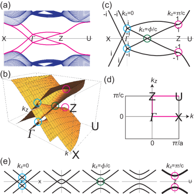
Figure 1: Band structure of the glided QSH insulator. (a) The band structure along the X$\Gamma$ZU line. The red curves near the Fermi level represent the surface state. (b) Bird’s eye’s views of the energy spectrum for the surface state in the $(k,k_{z})$ plane. There are two vertically placed Dirac cones at the $\Gamma$ point, representing the hourglass fermion surface state. The nonsymmorphic symmetry protected gap closing point is marked by a green circle. The Kramers (pseudo Kramers) doublets are marked by cyan (magenta) circles. (c) The energy spectrum based on the Dirac theory corresponding to (a), reproducing well the results for the surface state. The eigenvalues of the glide operator are shown. (c) The Brillouin zone for the surface, where X= $(\pi/a,0)$, $\Gamma=(0,0)$, Z=$(0,\pi/c)$, and U=$(\pi/a,\pi/c)$ in the $(k,k_{z})$ plane. Here, $a$ and $c$ are the lattice constants of the honeycomb lattice and the $k_{z}$ direction, respectively. (e) The band structure along the $k$ direction for various $k_{z}$.

I Introduction

Topological insulators are fascinating concept found in condensed matter physicsHasan ; Qi . They can be either genuine such as quantum-Hall and quantum-anomalous-Hall (QAH) insulatorsHaldane ; Chang or symmetry protected. Time-reversal symmetry (TRS) protected topological insulators such as quantum-spin-Hall (QSH) insulators evoke intense research on this topicKM ; B1 ; B2 . Later they are generalized to topological crystalline insulators, where the topology is protected by the crystalline symmetry such as the mirror symmetryTCI ; Hsieh ; Tanaka ; Dziawa ; Xu ; Robert ; Ando . However the symmetry is restricted to be symmorphic although some extension to combined symmetry is exploredAris .

Recently, topological crystalline insulators are generalized further to include the nonsymmorphic symmetry, and called nonsymmorphic topological crystalline insulatorsVan ; Para ; Fang ; Dong ; Young ; Watanabe ; Po ; BJYang ; Murakami ; Sch ; ShiozakiB ; Shiozaki ; Chen ; Varjas ; Po . A nonsymmorphic topological insulator was predicted in KHgSb by first-principles calculationsHour ; Coho and experimentally observed by ARPES (Angle-Resolved PhotoEmisison Spectroscopy)KHg in the same material soon after. A prominent feature is that there emerges entirely a new surface state called ”hourglass fermion”. It consists of four bands, in which two bands cross along a high-symmetry line. This band crossing is protected by the nonsymmorphic symmetry. The constructed effective theory is comprised of complicated forms based on three orbitals of Sb and one orbital of Hg, and is applicable only in the vicinity of the certain high-symmetry pointsHour ; Coho .

In this paper, motivated by these worksHour ; Coho ; KHg , we propose a tight-binding model producing a hourglass fermion surface state [Fig.1] by the stacked helical edge states with the nonsymmorphic symmetry. They are realized by the binary stacking of the QSH insulators. The unit cell contains two layers of the QSH insulators, which results in a Z₂-trivial insulator with respect to the TRS. Each layer has helical edge modes; two right-going edge modes with up spin and two left-going edge modes with down spin. In general, these helical edge modes are gapped out by interlayer couplings. Nevertheless, an interesting feature is that a gap closing is assured even after introducing the interlayer couplings provided the nonsymmorphic symmetry is intact, leading to a hourglass fermion surface state in the stacked system. (Let us call it the hourglass state for simplicity.) To generate such a state, we first make a half lattice transformation $\overline{t}_{z}=e^{-ick_{z}/2}$, where $c$ is a lattice constant along the $\mathbf{z}$ directionYoung ; Shiozaki ; Fang ; Coho . Then we perform an additional mirror reflection. The combined operation is the glide operation. We also derive the glided Dirac theory as an effective theory for the hourglass state. It accounts for the above mentioned properties of the hourglass state analytically [Fig.1(c)]. We also investigate the breaking of the hourglass state by introducing perturbations possessing various symmetries. Our results show that the hourglass state is universal in the helical edge system with the nonsymmorphic symmetry.

II Glided QAH insulator

We start with an explicit construction of a spinless tight-binding model possessing a nonsymmorphic symmetry protected surface state. We propose to stack the QAH insulators so as to preserve the nonsymmorphic symmetry. The QAH insulator is described by the Haldane HamiltonianHaldane ,

$$\hat{H}_{\text{QAH}}=-t\sum_{\left\langle i,j\right\rangle}c_{i}^{\dagger}c_{j}+i\frac{\lambda_{\text{H}}}{3\sqrt{3}}\sum_{\left\langle\!\left\langle i,j\right\rangle\!\right\rangle}\nu_{ij}c_{i}^{\dagger}c_{j},$$ (1)

where $\left\langle\!\left\langle i,j\right\rangle\!\right\rangle$ run over all the next-nearest neighbor hopping sites and $\nu_{ij}=\left(\vec{d}_{i}\times\vec{d}_{j}\right)/\left|\vec{d}_{i}\times\vec{d}_{j}\right|$ with $\vec{d}_{i}$ and $\vec{d}_{j}$ the two nearest bonds connecting the next-nearest neighbors. The first term represents the usual nearest-neighbor hopping on the honeycomb lattice with the transfer energy $t$ and the second term represents the Haldane interaction with the strength $\lambda_{\text{H}}$. We propose the glided QAH insulator model, which is $\hat{H}_{\text{gQAH}}=\sum_{\mathbf{k}}H_{\text{gQAH}}\left(\mathbf{k}\right)c_{\mathbf{k}}^{\dagger}c_{\mathbf{k}}$ in the momentum space with

$$H_{\text{gQAH}}\left(\mathbf{k}\right) =H_{\text{QAH}}\left(k_{x},k_{y}\right)+G_{\alpha}\left(k_{z}\right)H_{\text{H}}\left(k_{x},k_{y}\right)G_{\alpha}\left(k_{z}\right)^{-1}$$

$$+\Gamma_{\text{QAH}}\left(k_{z}\right),$$ (2)

where $\alpha=x$ or $y$. Hereafter we choose $\alpha=x$ for definiteness. The first term is the Haldane Hamiltonian for the $A$ layer. The second term is the Hamiltonian for the $B$ layer constructed with the aid of the glide operator $G_{x}\left(k_{z}\right)$. The third term $\Gamma_{\text{QAH}}\left(k_{z}\right)$ represents the interlayer coupling preserving the nonsymmorphic symmetry.

The glide operation $G_{x}\left(k_{z}\right)$ is the successive operation of the half translation $\overline{t}_{z}$ and the mirror operation $M_{x}$. The mirror operation $M_{x}$ is just the reflection $\mathcal{R}_{x}$ in the absence of the spin, $\mathcal{R}_{x}:\left(k_{x},k_{y},k_{z}\right)\rightarrow\left(-k_{x},k_{y},k_{z}\right)$. It is given byFang ; Sch ; Shiozaki

$$G_{x}\left(k_{z}\right)=e^{-i\frac{ck_{z}}{2}}\Omega(k_{z})\mathcal{R}_{x}$$ (3)

with

$$\Omega(k_{z})=\cos\frac{ck_{z}}{2}\eta_{x}+\sin\frac{ck_{z}}{2}\eta_{y}.$$ (4)

Here, $\eta_{\alpha}$ are the Pauli matrices for the layer degrees of freedom (pseudospin). It follows that $G_{x}^{2}\left(k_{z}\right)=e^{-ick_{z}}\eta_{0}$.

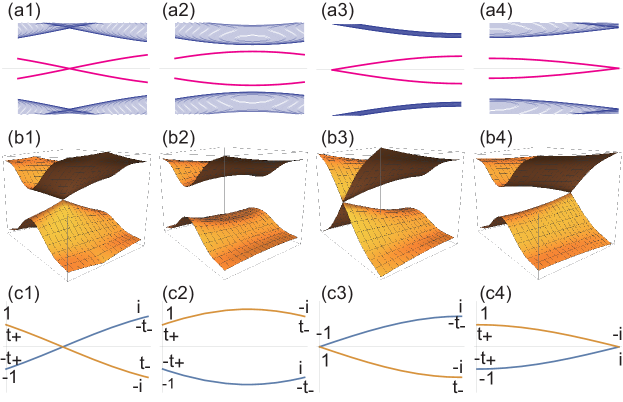
Figure 2: Band structure of the glided QAH insulator model. The band structure along the line $k=0$ for $0\leq ck_{z}\leq\pi$: (a1) $t_{+}t_{-}<0$, (a2) $t_{+}t_{-}>0$, (a3) $t_{+}=0$, and (a4) $t_{-}=0$. The red curves near the Fermi level represent the surface states. (b1)$\sim$ (b4) Bird’s eye’s views of the energy spectrum for the surface states corresponding to (a1)$\sim$(a4) in the $(k,k_{z})$ plane. (c1)$\sim$(c4) The energy spectrum based on the Dirac theory corresponding to (a1)$\sim$ (a4). The eigenvalues of the glide operator are shown.

We determine the term $\Gamma_{\text{QAH}}\left(k_{z}\right)$. The only condition imposed on it is $G_{x}\left(k_{z}\right)\Gamma_{\text{QAH}}\left(k_{z}\right)G_{x}^{-1}\left(k_{z}\right)=\Gamma_{\text{QAH}}\left(k_{z}\right)$, or

$$\Omega(k_{z})\Gamma_{\text{QAH}}\left(k_{z}\right)\Omega^{-1}(k_{z})=\Gamma_{\text{QAH}}\left(k_{z}\right).$$ (5)

The simplest solution is obviously given by

$$\Gamma_{\text{QAH}}\left(k_{z}\right)=f\left(k_{z}\right)\Omega(k_{z})$$ (6)

with an arbitrary c-number function $f\left(k_{z}\right)$. We choose $f\left(k_{z}\right)$ to represent the coupling between the adjacent layers, or

$$\Gamma_{\text{QAH}}\left(k_{z}\right)=\left(t_{+}\cos\frac{ck_{z}}{2}+t_{-}\sin\frac{ck_{z}}{2}\right)\Omega(k_{z}),$$ (7)

where $t_{+}$ ($t_{-}$) represents an ordinary (skew) interlayer hopping amplitude.

The glide operation $G_{x}\left(k_{z}\right)$ acts on the Hamiltonian as

$$G_{x}\left(k_{z}\right)H_{\text{gQAH}}\left(k_{x},k_{y},k_{z}\right)G_{x}^{-1}\left(k_{z}\right)=H_{\text{gQAH}}\left(-k_{x},k_{y},k_{z}\right).$$ (8)

We focus on the surface made of the edges of each layers, where $k_{y}=0$ and we set $k=k_{x}$.

It follows from Eq.(8) that the glide operation commutes with the Hamiltonian for the glide invariant plane $k=0$,

$$\left[H_{\text{gQAH}}\left(0,k_{z}\right),G_{x}\left(k_{z}\right)\right]=0.$$ (9)

The operation of $G_{x}\left(k_{z}\right)$ twice results in the one-unit cell translation. The eigen function $\left|\psi^{\pm}\left(0,k_{z}\right)\right\rangle$ satisfies

$$G_{x}\left|\psi^{\pm}\left(0,k_{z}\right)\right\rangle=g_{\pm}\left(k_{z}\right)\left|\psi^{\pm}\left(0,k_{z}\right)\right\rangle.$$ (10)

The eigenvalues are

$$g_{\pm}\left(k_{z}\right)=\pm e^{-ick_{z}/2}$$ (11)

since $G_{x}^{2}\left(k_{z}\right)=e^{-ick_{z}}\eta_{0}$. Especially $g_{\pm}\left(0\right)=\pm 1$, $g_{\pm}\left(\pi/c\right)=\pm i$. All bands on the high-symmetry line $k=0$ is labeled by the eigenvalues of $G_{x}$. We show the glide eigenvalues $g_{\pm}\left(k_{z}\right)$ in Figs.2 (c1)$\thicksim$(c4).

We plot the band structure along the $k_{z}$ axis in Figs.2(a1)$\thicksim$(A4) for typical values of $t_{\pm}$. The isolated curves marked in red represent the surface modes. They are present between the bulk gap. We show the bird’s eye’s views of the band structure of the surface modes in the $(k,k_{z})$ plane in Figs.2(b1)$\thicksim$(b4). There are four types of the surface modes depending on $t_{+}$ and $t_{-}$. They are classified as follows:
1) When $t_{+}t_{-}<0$ they touch each other at the Fermi level at a certain point $(0,k_{z}^{0})$.
2) When $t_{+}t_{-}>0$, they never touch.
3) When $t_{+}=0$, they touch at $(0,0)$.
4) When $t_{-}=0$, they touch at $(0,\pi/c)$.
This classification is made clear based on the effective theory valid near the Fermi level, as we see soon.

III Glided Dirac theory of chiral edges

We construct the Dirac theory in order to obtain deeper understanding of the surface state. The chiral edge state of the glided QAH insulator is given by $H_{0}=vk\eta_{z}$ with $v\propto\lambda_{\text{H}}$ and $G_{x}\eta_{z}G_{x}^{-1}=-\eta_{z}$. On the other hand it is impossible to take the continuum limit in the $k_{z}$ direction. Hence the Hamiltonian for the stacked chiral edges with the nonsymmorphic symmetry is given by

$$H_{\text{gQAH}}=vk\eta_{z}+\Gamma_{\text{QAH}}\left(k_{z}\right),$$ (12)

together with Eq.(7). The energy spectrum reads

$$E_{\pm}\left(k,k_{z}\right)=\pm\sqrt{v^{2}k^{2}+\left(t_{+}^{2}+t_{-}^{2}\right)\sin^{2}\frac{ck_{z}-\phi}{2}},$$ (13)

where $\tan\frac{\phi}{2}=-t_{-}/t_{+}$. Especially we find

$$E_{\pm}\left(0,0\right)=\pm t_{+},\qquad E_{\pm}\left(0,\pi/c\right)=\pm t_{-}.$$ (14)

We plot the energy spectrum in Figs.2(c1)$\thicksim$ (c4), which agrees with the result in Figs.2(a1)$\thicksim$(a4) determined by the tight-binding model remarkable well.

The above mentioned classification of the surface modes is simply derived from the analytic formula Eq.(13). In particular, by solving $E_{\pm}\left(k,k_{z}\right)=0$, we find $\left(k,k_{z}\right)=(0,\phi/c)$, which is the gap closing point in Fig.2(b1). First, the appearance of the gapless modes is protected by the nonsymmorphic symmetry. Second, they appear at the same point in the $\left(k,k_{z}\right)$ plane due to the chiral symmetry,

$$CH_{\text{gQAH}}(k,k_{z})C^{-1}=-H_{\text{gQAH}}(-k,k_{z}),$$ (15)

where $C=\eta_{z}$ is the chiral operator. We can check $C\Omega(k_{z})C^{-1}=-\Omega(k_{z})$ for Eq.(4), from which the relation Eq.(15) follows.

IV Glided QSH insulator

We proceed to introduce the spin degrees of freedom. We construct the tight-binding model describing the glided helical edge by stacking the QSH insulators. For definiteness we choose the Kane-Mele modelKM to describe the QSH insulator in each layer,

$$\hat{H}_{\text{QSH}}=-t\sum_{\left\langle i,j\right\rangle s}c_{is,t}^{\dagger}c_{js,t}+i\frac{\lambda_{\text{SO}}}{3\sqrt{3}}\sum_{\left\langle\!\left\langle i,j\right\rangle\!\right\rangle s}s\nu_{ij}c_{is,t}^{\dagger}c_{js,t},$$ (16)

where $s=\pm$ is the spin index. We propose the glided QSH insulator model by

$$H_{\text{gQSH}}\left(\mathbf{k}\right) =\Gamma_{\text{QSH}}\left(k_{z}\right)+H_{\text{QSH}}\left(k_{x},k_{y}\right)$$

$$+G_{x}\left(k_{z}\right)TH_{\text{QSH}}\left(k_{x},k_{y}\right)T^{-1}G_{x}\left(k_{z}\right)^{-1}.$$ (17)

The term $\Gamma_{\text{QSH}}\left(k_{x},k_{y}\right)$ represents the interlayer coupling preserving the nonsymmorphic symmetry and the TRS.

The TRS is described by the operator $T=i\sigma_{y}K$ with $K$ the complex conjugation. It is an antiunitary operator. The operation $G_{x}\left(k_{z}\right)$ is the successive operation of the half translation $t\left(k_{z}\right)$ and the mirror operation $M_{x}$. The mirror operation is the composite operation of the reflection $\mathcal{R}_{x}$ and the spin reversion in the presence of the spin. Thus,

$$G_{x}\left(k_{z}\right)=i\sigma_{x}\otimes e^{-i\frac{ck_{z}}{2}}\Omega(k_{z})\mathcal{R}_{x},$$ (18)

where $\sigma_{\alpha}$ is the Pauli matrix for the spin, and $\Omega(k_{z})$ given by Eq.(4) involves the pseudospin. It follows that $G_{x}^{2}\left(k_{z}\right)=-e^{-ick_{z}}\sigma_{0}\otimes\eta_{0}$. The sign is negative due to the $2\pi$ spin rotation, which is different from the spinless case.

We determine $\Gamma_{\text{QSH}}\left(k_{z}\right)$. We consider the simplest candidates $t_{+}\cos\frac{ck_{z}}{2}\sigma_{\alpha}\otimes\Omega(k_{z})$ and $t_{-}\sin\frac{ck_{z}}{2}\sigma_{\alpha}\otimes\Omega(k_{z})$ describing the ordinary and skew interlayer hoppings as in the case of the glided QAH insulator model. We choose the relevant terms by requiring the symmetry property. Since the Kane-Mele model has the TRS, we require the TRS also for $\Gamma_{\text{QSH}}\left(k_{z}\right)$. Namely, we require both $T\Gamma_{\text{QSH}}\left(k_{z}\right)T^{-1}=\Gamma_{\text{QSH}}\left(-k_{z}\right)$ and $G_{x}\left(k_{z}\right)\Gamma_{\text{QSH}}\left(k_{z}\right)G_{x}^{-1}\left(k_{z}\right)=\Gamma_{\text{QSH}}\left(k_{z}\right)$. The only possible term is

$$\Gamma_{\text{QSH}}\left(k_{z}\right)=\left(t_{+}\sigma_{0}\cos\frac{ck_{z}}{2}+t_{-}\sigma_{x}\sin\frac{ck_{z}}{2}\right)\otimes\Omega\left(k_{z}\right).$$ (19)

We obtain

$$G_{x}\left(k_{z}\right)H_{\text{gQSH}}\left(k_{x},k_{y},k_{z}\right)G_{x}^{-1}\left(k_{z}\right)=H_{\text{gQSH}}\left(-k_{x},k_{y},k_{z}\right).$$ (20)

We focus on the surface made of the edges of each layers, where $k_{y}=0$ and we set $k=k_{x}$.

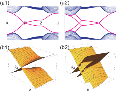
Figure 3: Band structure of the glided QSH insulator model for $t_{+}t_{-}=0$. The band structure along the X$\Gamma$ZU line for (a1) $t_{+}=0$, and (a2) $t_{-}=0$. The red curves near the Fermi level represent the surface states. (b1),(b2) Bird’s eye’s views of the energy spectrum for the surface states.

We plot the band structure based on the tight-binding model Eq.(17) together with Eq.(19) for $t_{+}t_{-}\neq 0$ in Fig.1 and for $t_{+}t_{-}=0$ in Fig.3. First of all, the energy dispersion for the surface mode [Fig.1(a)] reproduces excellently the results obtained by the DFT theoryHour and the ARPES experimentKHg . It is remarkable that the hourglass state emerges due to this interlayer hopping [Fig.1(b)]. It should be noted that the band crossing occurs irrespective to the sign of $t_{+}t_{-}$ since these four bands connect between $k_{z}=0$ and $k_{z}=\pi/c$ in contrast to the spinless case. There is the Kramers degeneracy at the time-reversal invariant momentum $\Gamma$ ($k=0$ and $k_{z}=0$). On the other hand, there is a double-fold degeneracy for all $k$ with $k_{z}=\pi/c$. This is the pseudo-Kramers degeneracy of the operatorHour ; Coho $G_{x}\left(k_{z}\right)T$ at $k_{z}=\pi/c$ due to the fact $\left(G_{x}\left(\pi/c\right)T\right)^{2}=-1$. Namely, the anti-unitary operator $G_{x}\left(\pi/c\right)T$ acts like the time-reversal symmetry and assures the pseudo-Kramers doublet.

When $t_{+}=0$, the two Kramers degeneracies at $E=\pm t_{+}$ with $k_{z}=0$ become identical and becomes a four-fold degenerated state, whose band structure is plotted in Fig.3(a1) and (b1). On the other hand, when $t_{-}=0$, the two pseudo-Kramers degeneracies at $E=\pm t_{-}$ with $k_{z}=\pi/c$ becomes identical and becomes to a four-fold degenerated state, whose band structure is plotted in Fig.3(a2) and (b2).

V Glided Dirac theory of helical edges

We can prove these properties of the band structure depending on $t_{+}$ and $t_{-}$ analytically based on the Dirac theory. The Dirac theory is derived to describe the surface state,

$$H_{\text{gQSH}}\left(k,k_{z}\right)=vk\sigma_{z}+\Gamma_{\text{QSH}}\left(k_{z}\right)$$ (21)

together with Eq.(19). The energy spectrum is given by

$$E\left(k,k_{z}\right)=\pm\sqrt{\left(\sqrt{v^{2}k^{2}+\left(t_{+}\sin\frac{ck_{z}}{2}\right)^{2}}\pm t_{-}\cos\frac{ck_{z}}{2}\right)^{2}}.$$ (22)

We plot the energy spectrum along the X$\Gamma$ZU line in Fig.1 (c). This analytical result reproduces remarkably well the spectrum obtained based on the tight-binding model [Fig.1(a)], the DFT theoryHour and the ARPES experimentKHg . Typical featues read as follows:

(i) The energy spectrum along the $\Gamma$Z line ($k=0$) is given by $E\left(0,k_{z}\right)$: The gap closes at $\tan\frac{ck_{z}}{2}=\pm t_{0}/t_{x}$. This band crossing is protected by the nonsymmorphic symmetry and the chiral symmetry as in the case of the spinless model, where the glide eigenvalue is given by $g_{\pm}\left(k_{z}\right)=\pm ie^{-ick_{z}/2}$ and the chiral operator is given by $C=\sigma_{x}\eta_{z}$.

(ii) Along the ZU line ($k_{z}=\pi/c$), the energy spectrum is given by $E_{\pm}\left(k,\pi/c\right)$ with the double-fold degeneracy for all $k$, which is the pseudo-Kramers doublet as discussed in the tight-binding theory. The glide eigenvalues are $g_{x}\left(\pi/c\right)=\pm 1$, as plotted in Fig.1(c).

(iii) Along the $\Gamma$X line ($k_{z}=0$), the energy spectrum is given by the four linear edge states; $E_{\pm}\left(k,0\right)=vk\pm t_{0},-vk\pm t_{0}$. Each edge states are index by the glide eigenvalue of $g_{x}\left(0\right)=\pm i$, as plotted in Fig.1(c). There are the Kramers degeneracy at the time-reversal invariant momentum $\Gamma$ ($k=0$ and $k_{z}=0$) with $E_{\pm}\left(0,0\right)=\pm t_{0}$. On the other hand, the energy splits for $k\neq 0$.

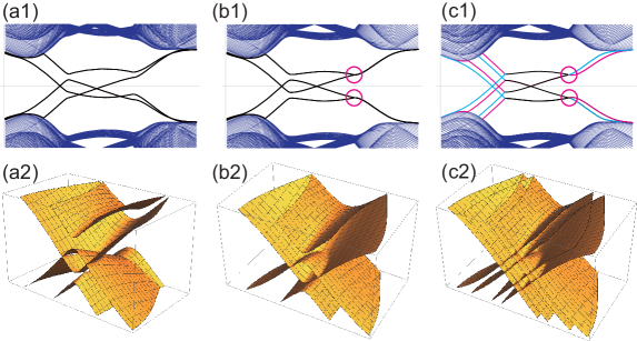
Figure 4: Hourglass fermion surface state along the X$\Gamma$ZU axis without the TRS. The TRS is broken by applying the magnetic field. (a) $B_{x}\neq 0$, (b) $B_{y}\neq 0$ and (c) $B_{z}\neq 0$. (a1)$\sim$(c1) The surface band structures become different between the both side of the edges. That of the one side is colored in magenta, while that of the other side is colored in cyan. (a2)$\sim$(c2) Bird’s eye’s views of the energy spectrum for the surface states.

VI Breaking the hourglass state

We apply external magnetic field to the sample by introducing the Zeeman coupling $\mathbf{B}\cdot\mathbf{\sigma}$. The band structures are illustrated in Fig.4, which are interpreted based on the symmetry as follows. When the magnetic field is along $y$ or $z$ direction, the $G_{x}T$ symmetry is preserved although the nonsymmorphic symmetry $G_{x}$ and the TRS are broken. As a result, while the pseudo-Kramers degeneracy at $k_{z}=\pi/c$ is preserved, the Kramers degeneracy at $k_{z}=0$ is broken. Although the band crossing is preserved even after the introduction of the additional terms $\sigma_{y}$ or $\sigma_{z}$, it is not protected by the nonsymmorphic symmetry $G_{x}$. The connection of the edge states along $k_{z}=0$ line is different between $B_{y}\sigma_{y}$ and $B_{z}\sigma_{z}$, as shown in Fig.4(b) and (c). We note that the degeneracy between the both sides of the edges is broken due to the $\sigma_{z}$ term, where $8$ bands emerge. The Zeeman field is opposite between the two sides of the surfaces, which results in the difference between the surface band structure between the both sides of the surfaces. On the other hand, $B_{x}\sigma_{x}$ breaks both the $G_{x}T$ and $T$ symmetries, which results in the breaking both of the Kramers and pseudo Kramers degeneracies, as shown in Fig.4(a). The band structure is not symmetric with respect to the Fermi energy. This is because that the chiral symmetry $C=\sigma_{x}\eta_{z}$ is also broken, which results in the shift of the gap closing point away from the Fermi energy with $B_{x}\sigma_{x}$. However the band crossing is protected by the nonsymmorphic symmetry $G_{x}$ since the nonsymmorphic symmetry is preserved.

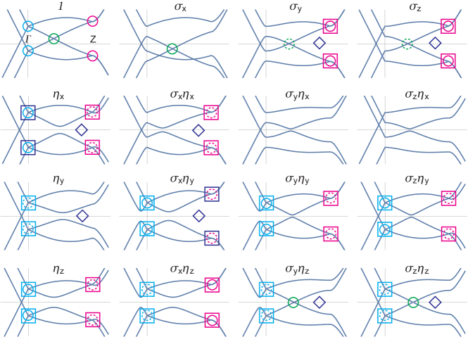
Figure 5: Energy spectrum of the hourglass fermion with the perturbation $V$ based on the Dirac theory. The band crossings protected by the glide symmetry $G_{x}$ occur for $V\propto 1$, $\sigma_{x}$, $\sigma_{y}\eta_{z}$, $\sigma_{z}\eta_{z}$ and are marked by solid green circles, while those which are not protected by $G_{x}$ are marked by dotted green circles. The energy degeneracies protected by the time-reversal symmetry $T$ occur at the $\Gamma$ point for $V\propto 1$, $\eta_{x}$, $\sigma_{x}\eta_{y}$, $\sigma_{y}\eta_{y}$, $\sigma_{z}\eta_{y}$, $\eta_{z}$ and are denoted by solid cyan circles, while those which are not protected by $T$ are marked by the dotted cyan circles. The energy degeneracies protected by the local chiral symmetry $C_{0}$ occurs for $V\propto\eta_{y}$, $\sigma_{x}\eta_{y}$, $\sigma_{y}\eta_{y}$, $\sigma_{z}\eta_{y}$, $\eta_{z}$, $\sigma_{x}\eta_{z}$, $\sigma_{y}\eta_{z}$, $\sigma_{z}\eta_{z}$ and are marked by solid cyan squares. The energy degeneracies at the $Z$ point protected by the time-reversal nonsymmorphic symmetry $G_{x}T$ occurs for $V\propto 1$, $\sigma_{y}$, $\sigma_{z}$, $\ \sigma_{x}\eta_{z}$ are marked by solid magenta circles, while those which are not protected by $G_{x}T$ are marked by dotted magenta circles. The energy degeneracies protected by the local chiral symmetry $C_{\pi}$ occurs for $V\propto\sigma_{y}$, $\sigma_{z}$, $\eta_{x}$, $\sigma_{x}\eta_{x}$, $\sigma_{y}\eta_{y}$, $\sigma_{z}\eta_{y}$, $\eta_{z}$, $\sigma_{x}\eta_{z}$ and are marked by solid magenta squares. The degeneracies occur due to the fact $V\propto H_{\text{gQSH}}$ at the $\Gamma$ point for $\eta_{x}$ and at the $Z$ point for $\sigma_{x}\eta_{y}$, and are marked by solid purple squares. Symmetric band structures along $E=0$ due to the chiral symmetry for $V\propto\sigma_{y}$, $\sigma_{x}\eta_{x}$, $\eta_{y}$, $\sigma_{z}\eta_{z}$ are marked by solid purple diamonds.

We further investigate how the band structures are modified by introducing perturbation terms of the form $V=V_{0}\sigma_{\alpha}\eta_{\beta}$. See Section VII for details. We illustrate the results in Fig.5, which are interpreted based on the symmetry as follows. The degeneracy at the $\Gamma$ and $Z$ points are well explained by the symmetry operations $T$ and $G_{x}T$. However it is interesting that there are degeneracies at the $\Gamma$ and $Z$ points which are not protected by these symmetries. In order to clarify these degeneracies we write down the Hamiltonian at the $\Gamma$ and $Z$ points,

$$H_{\text{gQSH}}\left(0,0\right)=t_{+}\sigma_{0}\eta_{x},\quad H_{\text{gQSH}}\left(0,\pi/c\right)=t_{-}\sigma_{x}\eta_{y}.$$ (23)

When $\left[H_{\text{gQSH}},V\right]\neq 0$, the energy spectrum of the Hamiltonian $H_{\text{gQSH}}+V$ is given by the two two-fold degenerate levels,

$$E=\pm\sqrt{t_{\pm}^{2}+V_{0}^{2}}.$$ (24)

On the other hand, when $\left[H_{\text{gQSH}},V\right]=0$, it is given by non-degenerate four levels,

$$E=\pm t_{\pm}\pm V_{0}.$$ (25)

Hence, the degeneracy is assured by $\left[H_{\text{gQSH}},V\right]\neq 0$. It is identical to the condition $\left\{H_{\text{gQSH}},V\right\}=0$, which is a local chiral symmetry, in the present case of $V=V_{0}\sigma_{\alpha}\eta_{\beta}$. The local chiral symmetry at the $\Gamma$ point is explicitly written as

$$C_{0}H\left(0,0\right)+H\left(0,0\right)C_{0}=0$$ (26)

with

$$C_{0}=\eta_{x},$$ (27)

which protects the symmetry along $E=0$ at the $\Gamma$ point, as marked by solid cyan squares in Fig.5. Similarly, the local chiral symmetry at the $Z$ point is explicitly written as

$$C_{\pi}H\left(0,\pi/c\right)+H\left(0,\pi/c\right)C_{\pi}=0$$ (28)

with

$$C_{\pi}=\sigma_{x}\eta_{y},$$ (29)

which protects the symmetry along $E=0$ at the $Z$ point, as marked by solid magenta squares in Fig.5. A exception occurs provided the perturbation term $V$ is proportional to $H_{\text{gQSH}}$, where the energy spectrum is given by the two two-fold degenerate levels,

$$E=t_{\pm}+V_{0},\quad-t_{\pm}-V_{0},$$ (30)

although the original Hamiltonian $H_{\text{gQSH}}$ and $V$ commute trivially, $\left[H_{\text{gQSH}},V\right]=0$. We mark this case by solid purple squares in Fig.5.

VII Symmetry analysis

We investigate the symmetry of the additional perturbation term $V$ and its effects on the band structure in detail, where $V$ is of the form

$$V=\sigma_{\alpha}\eta_{\beta}.$$ (31)

The glide symmetry $G_{x}$ is given by

$$G_{x}\left(k_{z}\right)=i\sigma_{x}\otimes e^{-i\frac{ck_{z}}{2}}\Omega(k_{z})\mathcal{R}_{x},$$ (32)

and characterized by the action

$$G_{x}\left(k_{z}\right)H\left(k,k_{z}\right)G_{x}^{-1}\left(k_{z}\right)=H\left(-k,k_{z}\right)$$ (33)

on the unperturbed Hamiltonian $H\left(k,k_{z}\right)$. The perturbation term $V$ is classified by the glide symmetry as

$$G_{x}\left(k_{z}\right)V\left(-k,k_{z}\right)G_{x}^{-1}\left(k_{z}\right)=\varepsilon^{G_{x}}V\left(-k,k_{z}\right),$$ (34)

where $\varepsilon^{G_{x}}=\pm 1$; we give $\varepsilon^{G_{x}}$ for various $V$ in Table I. The glide symmetry is preserved (violated) for $\varepsilon^{G_{x}}=1$ ($-1$). The glide symmetry protects the gap closing for the perturbations $1$, $\sigma_{x}$, $\sigma_{y}\eta_{z}$, $\sigma_{z}\eta_{z}$, as marked by solid green circles in Fig.5.

The TRS $T$ is defined by

$$TH\left(k,k_{z}\right)T^{-1}=H\left(-k,-k_{z}\right)$$ (35)

with

$$T=i\sigma_{y}K.$$ (36)

The TRS protects the degeneracies at $k=0$ and $k_{z}=0$ for the perturbations $1$, $\eta_{x}$, $\sigma_{x}\eta_{y}$, $\sigma_{y}\eta_{y}$, $\sigma_{z}\eta_{y}$, $\eta_{z}$, as marked by solid cyan circles in Fig.5. The perturbation term $V$ is classified by the TRS as

$$TV\left(k,k_{z}\right)T^{-1}=\varepsilon^{T}V\left(-k,-k_{z}\right),$$ (37)

where $\varepsilon^{T}=\pm 1$; we give $\varepsilon^{T}$ for various $V$ in Table I.

$1$

$\sigma_{x}$

$\sigma_{y}$

$\sigma_{z}$

$\eta_{x}$

$\sigma_{x}\eta_{x}$

$\sigma_{y}\eta_{x}$

$\sigma_{z}\eta_{x}$

$\eta_{y}$

$\sigma_{x}\eta_{y}$

$\sigma_{y}\eta_{y}$

$\sigma_{z}\eta_{y}$

$\eta_{z}$

$\sigma_{x}\eta_{z}$

$\sigma_{y}\eta_{z}$

$\sigma_{z}\eta_{z}$

$T$

$+$

$-$

$-$

$-$

$+$

$-$

$-$

$-$

$-$

$+$

$+$

$+$

$+$

$-$

$-$

$-$

$G_{x}$

$+$

$+$

$-$

$-$

X

X

X

X

X

X

X

X

$-$

$-$

$+$

$+$

$G_{x}T$

$+$

$-$

$+$

$+$

X

X

X

X

X

X

X

X

$-$

$+$

$-$

$-$

$G_{y}$

$+$

$-$

$+$

$-$

X

X

X

X

X

X

X

X

$-$

$+$

$-$

$+$

$C$

$-$

$-$

$+$

$+$

$+$

$+$

$-$

$-$

$+$

$+$

$-$

$-$

$-$

$-$

$+$

$+$

$C_{0}$

$-$

$-$

$-$

$-$

$-$

$-$

$-$

$-$

$+$

$+$

$+$

$+$

$+$

$+$

$+$

$+$

$C_{\pi}$

$-$

$-$

$+$

$+$

$+$

$+$

$-$

$-$

$-$

$-$

$+$

$+$

$+$

$+$

$-$

$-$

Table 1: The sign of the symmetry operations $\varepsilon^{S}=\pm$ with $S=T,G_{x},G_{x}T,C,C_{0},C_{\pi}$. X denotes that there is no symmetry. $\varepsilon^{S}=+$ ($-$) indicates that the symmetry $S$ is preserved (violated) by the perturbation,.

The time-reversal glide symmetry $G_{x}\left(k_{z}\right)T$ is defined by the product of the glide and time-reversal symmetries as

$$\left(G_{x}\left(k_{z}\right)T\right)H\left(k,k_{z}\right)\left(G_{x}\left(k_{z}\right)T\right)^{-1}=H\left(k,-k_{z}\right).$$ (38)

The signs of the combined operation $\varepsilon^{G_{x}T}$ are given by the product of the glide and the time-reversal symmetry

$$\varepsilon^{G_{x}T}=\varepsilon^{G_{x}}\varepsilon^{T}.$$ (39)

This symmetry is anti-unitary and leads to the pseudo-Kramers degeneracy at $Z$ point for the perturbations $1$, $\sigma_{y}$, $\sigma_{z}$, $\ \sigma_{x}\eta_{z}$, as marked by solid magenta circles in Fig.5.

The particle-hole symmetry $P$ is defined by

$$P=i\sigma_{z}\eta_{z}K$$ (40)

with

$$PH\left(k,k_{z}\right)P^{-1}=-H\left(-k,k_{z}\right).$$ (41)

The chiral symmetry $C$ is the product of the TRS and the PHS, and defined by

$$CH\left(k,k_{z}\right)+H\left(k,k_{z}\right)C=0$$ (42)

with

$$C=\sigma_{x}\eta_{z}.$$ (43)

The perturbation term $V$ is classified with by the chiral symmetry as

$$CV\left(k,k_{z}\right)+\varepsilon^{C}V\left(k,k_{z}\right)C=0,$$

where $\varepsilon^{C}=\pm 1$; we give $\varepsilon^{C}$ for various $V$ in Table I. The band is symmetric along $E=0$ if there is the chiral symmetry for the perturbations $\sigma_{y}$, $\sigma_{x}\eta_{x}$, $\eta_{y}$, $\sigma_{z}\eta_{z}$, as marked by solid purple diamonds in Fig.5. However it seems that there are many band structures which are symmetric along $E=0$, as marked in the dashed purple diamonds. In order to clarify this symmetry, we further define the local chiral symmetry $C_{0}$ at the $\Gamma$ point,

$$C_{0}H\left(0,0\right)+H\left(0,0\right)C_{0}=0$$ (44)

with

$$C_{0}=\eta_{x},$$ (45)

which protects the symmetry along $E=0$ at the $\Gamma$ point for the perturbations $\eta_{y}$, $\sigma_{x}\eta_{y}$, $\sigma_{y}\eta_{y}$, $\sigma_{z}\eta_{y}$, $\eta_{z}$, $\sigma_{x}\eta_{z}$, $\sigma_{y}\eta_{z}$, $\sigma_{z}\eta_{z}$, as marked by solid cyan squares in Fig.5. We note that $C_{0}$ is proportional to $H(0,0)$. The perturbation term $V$ is classified by the chiral symmetry as

$$C_{0}V+\varepsilon^{C_{0}}VC_{0}=0,$$ (46)

where $\varepsilon^{C_{0}}=\pm 1$; we give $\varepsilon^{C_{0}}$ for various $V$ in Table I. Similarly, we define the local chiral symmetry $C_{\pi}$ at the $Z$ point,

$$C_{\pi}H\left(0,\pi/c\right)+H\left(0,\pi/c\right)C_{\pi}=0$$ (47)

with

$$C_{\pi}=\sigma_{x}\eta_{y},$$ (48)

which protects the symmetry along $E=0$ at the $Z$ point for the perturbations $\sigma_{y}$, $\sigma_{z}$, $\eta_{x}$, $\sigma_{x}\eta_{x}$, $\sigma_{y}\eta_{y}$, $\sigma_{z}\eta_{y}$, $\eta_{z}$, $\sigma_{x}\eta_{z}$, as marked by solid magenta squares in Fig.5. We note that $C_{0}$ is proportional to $H(0,\pi/c)$. The perturbation term $V$ is classified by the chiral symmetry as

$$C_{\pi}V+\varepsilon^{C_{\pi}}VC_{\pi}=0$$ (49)

where $\varepsilon^{C_{\pi}}=\pm 1$; we given $\varepsilon^{C_{\pi}}$ for various $V$ in Table I.

VIII Discussion

We have demonstrated that the hourglass fermion surface state is well described by the glided QSH insulator model and the glided Dirac theory, where the degeneracy at the high-symmetry points are protected by the nonsymmorphic symmetry and the TRS. The symmetry with respect to the Fermi energy is protected by the chiral symmetry. We have shown that these degeneracies are lifted by applying magnetic field, which will be observable in ARPES experiments. Although the hourglass fermion surface state was found in a specific material, KHgSb, both theoretically and experimentally, our results show that it is universal in the helical edge system with the nonsymmorphic symmetry.

- (1) M. Z. Hasan and C. L. Kane, Rev. Mod. Phys. 82, 3045 (2010)
- (2) X.-L. Qi and S.-C. Zhang, Rev. Mod. Phys. 83, 1057 (2011)
- (3) F. D. M. Haldane, Phys. Rev. Lett. 61, 2015 (1988)
- (4) C.-Z. Chang. et.al., Sicence 340, 167 (2013)
- (5) C. L. Kane and E. J. Mele, Phys. Rev. Lett. 95, 146802 (2005): C. L. Kane and E. J. Mele, Phys. Rev. Lett. 95, 226801 (2005).
- (6) B. A. Bernevig, T. L. Hughes, S.-C. Zhang, Science, 314, 1757 (2006)
- (7) B. A. Bernevig and S.-C. Zhang, Phys. Rev. Lett. 96, 106802 (2006)
- (8) L. Fu, Phys. Rev. Lett. 106, 106802 (2011).
- (9) T. H. Hsieh, et.al, Nat. Commun. 3, 982 (2012).
- (10) Y. Tanaka, et.al., Nat. Phys. 8, 800 (2012).
- (11) P. Dziawa, et.al., Nat. Mater. 11, 1023 (2012).
- (12) S.-Y. Xu, et al., Nat. Commun. 3, 1192 (2012).
- (13) R.-J. Slager, A. Mesaros, V. Juricic, J. Zaanen, Nature Physics 9, 98?102 (2013)
- (14) Y. Ando and L. Fu, Annual Review of Condensed Matter Physics, 6, 361 (2015).
- (15) A. Alexandradinata, C. Fang, M. J. Gilbert, and B. A. Bernevig, Phys. Rev. Lett. 113, 116403 (2014)
- (16) C.-X. Liu, R.-X. Zhang, and B. K. VanLeeuwen, Phys. Rev. B 90, 085304 (2014).
- (17) S. A. Parameswaran, A. M. Turner, D. P. Arovos, and A. Vishwanath, Nat. Phys. 9, 299 (2013).
- (18) C. Fang and L. Fu, Phys. Rev. B 91, 161105 (2015).
- (19) X.-Y. Dong and C.-X. Liu, Phys. Rev. B 93, 045429 (2016)
- (20) S. M. Young and C. L. Kane, Phys. Rev. Lett. 115, 126803 (2015)
- (21) H. Watanabe, H. C. Po, A. Vishwanath, M. P. Zaletel, Proc. Natl. Acad. Sci. 112, 14551 (2015)
- (22) H. C. Po, H. Watanabe, M. P. Zaletel, A. Vishwanath, Sci. Adv. 2(4), e1501782 (2016)
- (23) B.-J. Yang, T. A. Bojesen, T. Morimoto, A. Furusaki, cond-mat/arXiv:1604.00843
- (24) H. Kim and S. Murakami, Phys. Rev. B 93, 195138 (2016)
- (25) Y. Z. Zhao, A. P. Schnyder, cond-mat/arXiv:1606.03698
- (26) K. Shiozaki, M. Sato and K. Gomi, Phys. Rev. B 91, 155120 (2015)
- (27) K. Shiozaki, M. Sato and K. Gomi, Phys. Rev. B 93, 195413 (2016)
- (28) Y. Chen, H.-S. Kim and H.-Y. Kee, Phys. Rev. B 93, 155140 (2016)
- (29) D. Varjas, F. de Juan and Y.-M. Lu, Phys. Rev. B 92, 195116 (2015)
- (30) P.-Y. Chang, O. Erten, P. Coleman, cond-maat/arXiv:1603.03435
- (31) Z. Wang, A. Alexandradinata, R. J. Cava and B. A. Bernevig. Nature 532, 189 (2016)
- (32) A. Alexandradinata, Z. Wang and B. A. Bernevig, Phys. Rev. X 6, 021008 (2016)
- (33) J.-Z. Ma, et. al., cond-mat/arXiv:1605.06824