Quantized chiral magnetic current
from reconnections of magnetic flux

Abstract

We introduce a new mechanism for the chiral magnetic effect that does not require an initial chirality imbalance. The chiral magnetic current is generated by reconnections of magnetic flux that change the magnetic helicity of the system. The resulting current is entirely determined by the change of magnetic helicity, and it is quantized.

The chiral magnetic effect (CME) is the generation of electric current induced by the chirality imbalance in the presence of a magnetic field Kharzeev:2004ey ; see Ref. Kharzeev:2013ffa for a review and references to related works. It is a macroscopic manifestation of the chiral anomaly Adler:1969gk ; Bell:1969ts . In most of the previous works reviewed in Refs. Kharzeev:2013ffa ; Kharzeev:2015kna ; Kharzeev:2015znc , the chirality imbalance is assumed to be generated by a topologically nontrivial background – for example, by parallel external electric and magnetic fields, or by the non-Abelian sphaleron transitions. In fact, recent experimental observations of the CME current in Dirac semimetals Li:2014bha ; Xiong2015 ; Huang2015 utilized parallel electric and magnetic fields. The magnetic field is usually introduced as an external background as well, even though a number of studies have addressed the role of the CME and anomaly-induced phenomena in the generation of magnetic helicity Joyce:1997uy ; Boyarsky:2011uy ; Tashiro:2012mf ; Tuchin:2014iua ; Manuel:2015zpa . For example, recently it was pointed out that the CME leads to a self-similar inverse cascade of magnetic helicity Hirono:2015rla ; Yamamoto:2016xtu .

In this Letter, we do not assume the presence of a chirality imbalance generated by an external topological background – instead, we consider the chirality associated with the topology of the magnetic flux itself. Indeed, in the absence of magnetic monopoles, the lines of magnetic field have to be closed. For example, the field lines of a solenoid form an “unknot.” However, the topology of the magnetic flux can be more complicated – specifically, the magnetic flux can form a chiral knot. Magnetic reconnections can change the chirality of this knot and induce the imbalance of chirality in the system. Can this imbalance of chirality lead to the generation of the chiral magnetic current? We will show that the answer to this question is positive. The corresponding chiral magnetic current is quantized, and is completely determined by the knot invariants.

Our main result is the following formula for the generated current $\Delta\bm{J}$ along the loops $C_{i}$ of the magnetic flux in terms of the change $\Delta\mathcal{H}$ of the magnetic helicity, which is a topological measure of the knot (to be defined below):

$$\sum_{i}\oint_{C_{i}}\Delta\bm{J}\cdot d\bm{x}=-\frac{e^{3}}{2\pi^{2}}\Delta\mathcal{H},$$ (1)

where $e$ is the electric charge. Since $\Delta\mathcal{H}$ is an integer number times the flux squared, the CME current resulting from reconnections of the magnetic flux is quantized. The process illustrated in Fig. 1 shows the simplest realization of such currents. This unlinking of a link involves the topology change of the magnetic fluxes, which leads to the generation of CME currents (indicated by dotted arrows) on both tubes. The amount of integrated current over the tubes is given by the helicity change during the process, as quantified by Eq. (1).

Let us now present the derivation of Eq. (1). Consider a set of closed tubes of the magnetic flux, in the presence of massless fermions. Repeated reconnections performed on this set will yield a topologically nontrivial structure containing links and knots of the magnetic flux; see the upper figure of Fig. 1 for a simple example. A nontrivial topology can also be introduced by the twisting of a flux tube berger1984topological ; moffatt1990energy ; Ricca1992 ; moffatt1992helicity . A link $\mathcal{K}$ of $N$ knots of the magnetic flux tubes can be characterized by magnetic helicity $\mathcal{H}$ (an Abelian Chern-Simons 3-form) that can be decomposed as

$$\mathcal{H}(\mathcal{K})=\sum_{i}\mathcal{S}_{i}\varphi^{2}_{i}+2\sum_{i,j}\mathcal{L}_{ij}\varphi_{i}\varphi_{j},$$ (2)

where $\varphi_{i}$ is the magnetic flux of the $i$th closed tube, $\mathcal{S}_{i}$ is the Călugăreanu-White self-linking number, and $\mathcal{L}_{ij}$ is the Gauss linking number moffatt1990energy ; Ricca1992 ; moffatt1992helicity .

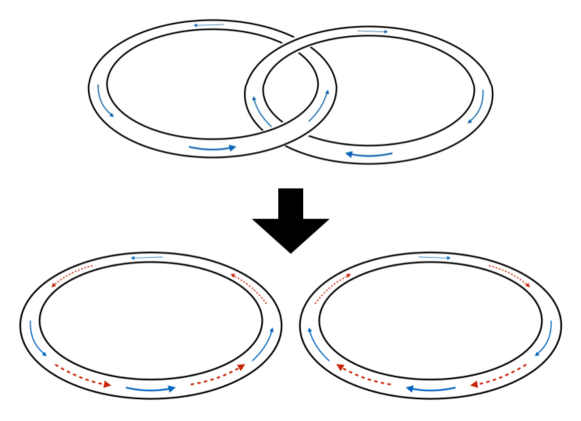
Figure 1: (Color online) Current generation associated with the unlinking of a simple link of two flux tubes. The solid arrows denote the directions of the magnetic field, and the dotted arrows indicate the directions of the generated CME currents.

The magnetic helicity can be changed either externally (flux reconnection) or internally (flux twist). Consider first the topology change of the flux tubes by a magnetic reconnection, as shown in Fig. 2. The reconnection leads to the change of the magnetic flux $\Phi$ flowing through the area encircled by each of the tubes. This change of the magnetic flux through Faraday’s induction generates an electric field parallel to the lines of the magnetic field,

$$\frac{d}{dt}\Phi=-\oint_{C_{1}}\bm{E}\cdot d\bm{x},$$ (3)

where $\Phi$ is the magnetic flux that penetrates the loop $C_{1}$. The change in the magnetic flux equals the flux contained inside the incoming tube, $\Delta\Phi=\varphi_{2}$. Faraday’s law allows us to write this change as

$$\Delta\Phi=\varphi_{2}=-\oint_{C_{1}}\left[\int_{0}^{\Delta t}\bm{E}(t)dt\right]\cdot d\bm{x},$$ (4)

where $\Delta t$ is the amount of time needed for the reconnection.

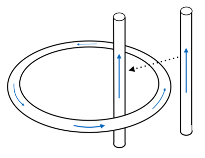
Figure 2: (Color online) A magnetic flux coming into a ring of another flux tube.

In this derivation we will assume that the magnetic field $B$ is strong, such that the magnetic length $(eB)^{-1/2}$ is small compared to the thickness of the flux tubes. The chiral fermions are then localized on lowest Landau levels (LLLs), and the system can be effectively treated as one dimensional. The relevant degrees of freedom are the Landau zero modes. Since the LLLs are not degenerate in spin, the handedness of a fermion is correlated with the direction of its motion (along or against the direction of the magnetic field). Our discussion will be analogous to the well-known description of the chiral anomaly in parallel electric and magnetic fields developed in Refs. Nielsen:1983rb ; Witten:1984eb .

The induced electric field changes the Fermi momenta of the left- and right-handed fermions:

$$\dot{\bm{p}_{F}}=\pm e\bm{E},$$ (5)

where the sign is plus (minus) for right- (left-)handed particles. This change of the Fermi momentum implies that the particles (antiparticles) of right- (left-)handed species are produced. The change in the Fermi momentum due to the magnetic reconnection is thus

$$\Delta\bm{p}_{F}=\pm\int_{0}^{\Delta t}e\bm{E}(t)dt.$$ (6)

Integrating this over the circumference of the tube,

$$\oint\Delta\bm{p}_{F}(s)\cdot d\bm{x}\equiv\int\Delta\bm{p}_{F}(s)\cdot\frac{d\bm{x}}{ds}ds=\pm e\oint_{C_{1}}\left[\int_{0}^{\Delta t}\bm{E}(t)dt\right]\cdot d\bm{x}=\mp e\varphi_{2},$$ (7)

where $s$ is a variable that parametrizes the position along the flux, and we have used Eq. (4) in the last equality. If $e\varphi_{2}$ is positive, there will be production of right-handed antiparticles, because the Fermi energy decreases for right-handed species. Since the density of states in (1+1) dimensions is given by $p_{F}/2\pi$, the number of produced antiparticles can be obtained as

$$\Delta\bar{N}_{R}=\frac{-\oint_{C_{1}}\Delta\bm{p}_{F}\cdot d\bm{x}}{2\pi}\times\frac{e\varphi_{1}}{2\pi}=\frac{e^{2}\varphi_{1}\varphi_{2}}{4\pi^{2}},$$ (8)

where $\varphi_{1}$ is the magnetic flux that forms the loop $C_{1}$, and $e\varphi_{1}/2\pi$ is the Landau degeneracy factor describing the transverse density of states in the cross section of the tube. On the other hand, for left-handed fermions, the Fermi energy increases, which means that particles are created; their number is given by

$$\Delta N_{L}=\frac{e^{2}\varphi_{1}\varphi_{2}}{4\pi^{2}}.$$ (9)

The particle production thus leads to the generation of currents of the left- and right-handed fermions, which are given by the charge density times velocity ($\pm 1$, respectively, for right- and left-handed currents) ,

$$\oint_{C_{1}}\Delta\bm{J}_{R}\cdot d\bm{x}=(-e)\times\Delta\bar{N}_{R}=-\frac{e^{3}\varphi_{1}\varphi_{2}}{4\pi^{2}},$$ (10)

where $(-e)$ is the charge of the antiparticle, and

$$\oint_{C_{1}}\Delta\bm{J}_{L}\cdot d\bm{x}=(-)\times e\times\Delta N_{L}=-\frac{e^{3}\varphi_{1}\varphi_{2}}{4\pi^{2}}.$$ (11)

The minus sign in Eq. (11) comes from the fact that the left-handed current flows in the opposite direction of the right-handed one. Therefore, the change in the total electric current is

$$\oint_{C_{1}}\Delta\bm{J}\cdot d\bm{x}=\oint_{C_{1}}\Delta\left[\bm{J}_{R}+\bm{J}_{L}\right]\cdot d\bm{x}=-\frac{e^{3}\varphi_{1}\varphi_{2}}{2\pi^{2}}.$$ (12)

The flux coming into the loop $C_{1}$ is a part of another loop, $C_{2}$. One can easily convince oneself that the contribution to the integrated current over $C_{2}$ is identical to that of $C_{1}$; therefore, we have

$$\sum_{i\in\{1,2\}}\oint_{C_{i}}\Delta\bm{J}\cdot d\bm{x}=\sum_{i\in\{1,2\}}\oint_{C_{i}}\Delta\left[\bm{J}_{R}+\bm{J}_{L}\right]\cdot d\bm{x}=-\frac{e^{3}}{2\pi^{2}}\times 2\varphi_{1}\varphi_{2}.$$ (13)

Here we have factored out the quantity $2\varphi_{1}\varphi_{2}$, which is nothing but the helicity change $\Delta\mathcal{H}$ in the process of switching moffatt1990energy ; Ricca1992 ; moffatt1992helicity , as is shown below. For two closed magnetic flux tubes, the magnetic helicity can be written as

$$\mathcal{H}=\int d^{3}x\ \bm{A}\cdot\bm{B}=2n\varphi_{1}\varphi_{2},$$ (14)

which can be illustrated as follows. When the tubes are very thin, $\bm{B}$ is localized along two closed curves, and the magnetic field can be written as

$$\bm{B}(\bm{x})=\varphi_{1}\int\frac{d\bm{X}_{1}(s)}{ds}\delta(\bm{x}-\bm{X}_{1}(s))ds+\varphi_{2}\int\frac{d\bm{X}_{2}(s)}{ds}\delta(\bm{x}-\bm{X}_{2}(s)),$$ (15)

where $\bm{X}_{1,2}(s)$ are the coordinates of the two closed curves with a parameter $s$. By plugging this expression into the definition of the magnetic helicity (14), we get

$$\mathcal{H}=\varphi_{1}\oint_{C_{1}}\bm{A}\cdot d\bm{X}_{1}+\varphi_{2}\oint_{C_{2}}\bm{A}\cdot d\bm{X}_{2}.$$ (16)

The line integrals count the fluxes, given by the Gauss linking number $n$ between $C_{1}$ and $C_{2}$:

$$\oint_{C_{1}}\bm{A}\cdot d\bm{X}_{1}=n\varphi_{2},\quad\oint_{C_{2}}\bm{A}\cdot d\bm{X}_{2}=n\varphi_{1}.$$ (17)

Thus, the magnetic helicity is expressed as

$$\mathcal{H}=2n\,\varphi_{1}\varphi_{2}.$$ (18)

Hence, the change in helicity, associated with the topology change of the curves, is given by the change in the linking number,

$$\Delta\mathcal{H}=2\left(\Delta n\right)\,\varphi_{1}\varphi_{2}.$$ (19)

Another way of changing the helicity is twisting. We can introduce a twist to a closed flux tube operationally, as in Ref. moffatt1990energy . When a twist of angle $2\pi\Delta n_{0}$ is introduced, the magnetic flux circled by a flux element $d\phi$ changes by

$$\Delta\Phi=\phi\ \Delta n_{0},$$ (20)

where $\phi$ is the flux inside. This change of flux induces a CME current on the flux element $d\phi$, the amount of which is given by (just as in the case of flux reconnection)

$$\int_{d\phi}\Delta\bm{J}\cdot d\bm{x}=-2\times\frac{e^{3}}{2\pi^{2}}\phi\ \Delta n_{0}d\phi=-\frac{e^{3}}{\pi^{2}}\phi\ \Delta n_{0}d\phi$$ (21)

where the factor 2 comes from the fact that the twisting of two flux tubes leads to the generation of currents in both of them in an equal amount. The induced current in the whole flux tube is obtained by integrating over the flux element,

$$\int_{C}\Delta\bm{J}\cdot d\bm{x}=\int d\phi\int_{d\phi}\Delta\bm{J}\cdot d\bm{x}=-\frac{e^{3}}{2\pi^{2}}\varphi^{2}\ \Delta n_{0}=-\frac{e^{3}}{2\pi^{2}}\ \Delta\mathcal{H}.$$ (22)

Here we have used the fact that the increment in helicity from twisting is $\Delta\mathcal{H}=\varphi^{2}\ \Delta n_{0}$, where $\varphi$ is the magnetic flux of the tube being twisted.

Equations (19) and (22), combined with the expression for the current (13) derived above, yield our main result (1).

A few comments are in order regarding the applicability of Eq. (1).

First, while deriving the formula, we have assumed that all of the flux tubes are contained within the volume of interest. The discussion can be naturally extended to the cases where the magnetic field is leaking from the volume. Once the boundary condition is fixed between volume A and volume B, the helicity difference can be determined with the knowledge of magnetic flux within volume A only (see Ref. berger1984topological ), and the derived formula applies to such cases as well.

Second, in the process of flux insertions, Ohmic currents can also be generated through Faraday’s law. Equation (1) holds only for the CME contribution to the current. The CME and Ohmic currents are different in nature and it is possible to distinguish them. The Ohmic current dissipates, and the CME current does not. If one waits long enough after a reconnection, the Ohmic contribution dies off and only the CME current remains.

Third, although our derivation of the formula is based on an assumption of the LLL approximation and the homogeneous magnetic field, the derived equation itself can hold on more general grounds, just as in the case of the chiral magnetic effect. The CME can be explained in terms of the spectral flow of the LLLs, but it can also be derived in hydrodynamics requiring the second law of thermodynamics Son:2009tf . Likewise, we believe that there exist other ways of derivation using, for example, chiral kinetic theory. Still, let us discuss the applicability of assumptions we made in deriving the formula (1). The discussed mechanism of the CME current generation resulting from the change of the topology of magnetic flux would operate in a plasma containing massless fermions, e.g. in the early Universe or in Dirac and Weyl semimetals. Thus, it seems reasonable to estimate the reconnection time scale within magnetohydrodynamics. In magnetohydrodynamics, the time evolution of the magnetic field is governed by the equation

$$\partial_{t}\bm{B}=\nabla\times(\bm{v}\times\bm{B})+\frac{1}{\sigma}\nabla^{2}\bm{B},$$ (23)

where $\sigma$ is the Ohmic conductivity and $\bm{v}$ is the fluid velocity. In order for a reconnection to occur, the conductivity has to be finite, because, in the infinite conductivity limit, the magnetic helicity is conserved and no reconnections of magnetic field lines are present. The time scale that controls magnetic reconnections is given by $t_{\rm rec}\sim\sigma L^{2}$, where $L$ is the typical length scale of the spatial inhomogeneity of the magnetic field. In order for the LLL approximation to be valid, $t_{\rm rec}$ should be much longer than the inverse of the energy difference between the Landau levels, $t_{\rm Landau}\sim 1/\sqrt{eB}$, namely $t_{\rm rec}\gg t_{\rm Landau}$. This can be written as

$$\sigma L^{2}\sqrt{eB}\gg 1.$$ (24)

As for the assumption about the homogeneity of the magnetic field, this is justified if the magnetic length $1/\sqrt{eB}$ is smaller than $L$, from which we obtain another condition,

$$L\sqrt{eB}\gg 1.$$ (25)

Hence, we expect that the scenario we describe in this Letter would be realized in a plasma with a massless fermion where the conditions (24) and (25) are satisfied.

To summarize, we have demonstrated that the chiral magnetic current can be generated without any initial chirality imbalance, by reconnections of the magnetic flux. This current is entirely determined by the integer change of the magnetic helicity and is, therefore, quantized. Our result has a number of implications – for example, it will affect the evolution of the magnetic helicity in chiral magnetohydrodynamics. Possible applications include the quark-gluon plasma in heavy-ion collisions, Dirac and Weyl semimetals, and primordial electroweak plasma produced after the big bang.

- (1) D. Kharzeev, Phys. Lett. B 633, 260 (2006) doi:10.1016/j.physletb.2005.11.075 [hep-ph/0406125]; D. Kharzeev and A. Zhitnitsky, Nucl. Phys. A 797, 67 (2007) doi:10.1016/j.nuclphysa.2007.10.001 [arXiv:0706.1026 [hep-ph]]; D. E. Kharzeev, L. D. McLerran and H. J. Warringa, Nucl. Phys. A 803, 227 (2008) doi:10.1016/j.nuclphysa.2008.02.298 [arXiv:0711.0950 [hep-ph]]; K. Fukushima, D. E. Kharzeev and H. J. Warringa, Phys. Rev. D 78, 074033 (2008) doi:10.1103/PhysRevD.78.074033 [arXiv:0808.3382 [hep-ph]].
- (2) D. E. Kharzeev, Prog. Part. Nucl. Phys. 75, 133 (2014) doi:10.1016/j.ppnp.2014.01.002 [arXiv:1312.3348 [hep-ph]].
- (3) S. L. Adler, Phys. Rev. 177, 2426 (1969). doi:10.1103/PhysRev.177.2426
- (4) J. S. Bell and R. Jackiw, Nuovo Cim. A 60, 47 (1969). doi:10.1007/BF02823296
- (5) D. E. Kharzeev, Ann. Rev. Nucl. Part. Sci. 65, 193 (2015) doi:10.1146/annurev-nucl-102313-025420 [arXiv:1501.01336 [hep-ph]].
- (6) D. E. Kharzeev, J. Liao, S. A. Voloshin and G. Wang, Prog. Part. Nucl. Phys. 88, 1 (2016) doi:10.1016/j.ppnp.2016.01.001 [arXiv:1511.04050 [hep-ph]].
- (7) Q. Li et al., Nature Phys. 12, 550 (2016) [arXiv:1412.6543 [cond-mat.str-el]].
- (8) J. Xiong et al., Science 350, 413 (2015) [arXiv:1503.08179].
- (9) X. Huang et al., Phys. Rev. X 5, 031023 (2015) [arXiv:1503.01304].
- (10) M. Joyce and M. E. Shaposhnikov, Phys. Rev. Lett. 79, 1193 (1997) doi:10.1103/PhysRevLett.79.1193 [astro-ph/9703005].
- (11) A. Boyarsky, J. Frohlich and O. Ruchayskiy, Phys. Rev. Lett. 108, 031301 (2012) doi:10.1103/PhysRevLett.108.031301 [arXiv:1109.3350 [astro-ph.CO]].
- (12) H. Tashiro, T. Vachaspati and A. Vilenkin, Phys. Rev. D 86, 105033 (2012) doi:10.1103/PhysRevD.86.105033 [arXiv:1206.5549 [astro-ph.CO]].
- (13) K. Tuchin, Phys. Rev. C 91, no. 6, 064902 (2015) doi:10.1103/PhysRevC.91.064902 [arXiv:1411.1363 [hep-ph]].
- (14) C. Manuel and J. M. Torres-Rincon, Phys. Rev. D 92, no. 7, 074018 (2015) doi:10.1103/PhysRevD.92.074018 [arXiv:1501.07608 [hep-ph]].
- (15) Y. Hirono, D. Kharzeev and Y. Yin, Phys. Rev. D 92, no. 12, 125031 (2015) doi:10.1103/PhysRevD.92.125031 [arXiv:1509.07790 [hep-th]].
- (16) N. Yamamoto, Phys. Rev. D 93, no. 12, 125016 (2016) doi:10.1103/PhysRevD.93.125016 [arXiv:1603.08864 [hep-th]].
- (17) M. A. Berger and G. B. Field, “The topological properties of magnetic helicity.” Journal of Fluid Mechanics 147 (1984): 133-148.
- (18) H. K. Moffatt, Nature 347, 367 (1990).
- (19) R. L. Ricca and H. K. Moffatt, “Topological Aspects of the Dynamics of Fluids and Plasmas” (Springer Netherlands, Dordrecht, 1992), chapter “The Helicity of a Knotted Vortex Filament”, pp. 225 - 236, ISBN 978-94-017-3550-6.
- (20) H. Moffatt and R. L. Ricca, in Proceedings of the Royal Society of London A: Mathematical, Physical and Engineering Sciences (The Royal Society, 1992), vol. 439, pp. 411-429.
- (21) H. B. Nielsen and M. Ninomiya, Phys. Lett. B 130, 389 (1983). doi:10.1016/0370-2693(83)91529-0
- (22) E. Witten, Nucl. Phys. B 249, 557 (1985). doi:10.1016/0550-3213(85)90022-7
- (23) D. T. Son and P. Surowka, Phys. Rev. Lett. 103, 191601 (2009) doi:10.1103/PhysRevLett.103.191601 [arXiv:0906.5044 [hep-th]].