Driven inelastic Maxwell gas in one dimension

Abstract

A lattice version of the driven inelastic Maxwell gas is studied in one dimension with periodic boundary conditions. Each site $i$ of the lattice is assigned with a scalar ‘velocity’, $v_{i}$. Nearest neighbors on the lattice interact, with a rate $\tau_{c}^{-1}$, according to an inelastic collision rule. External driving, occurring with a rate $\tau_{w}^{-1}$, sustains a steady state in the system. A set of closed coupled equations for the evolution of the variance and the two-point correlation is found. Steady state values of the variance, as well as spatial correlation functions, are calculated. It is shown exactly that the correlation function decays exponentially with distance, and the correlation length for a large system is determined. Furthermore, the spatio-temporal correlation $C(x,t)=\langle v_{i}(0)v_{i+x}(t)\rangle$ can also be obtained. We find that there is an interior region $-x^{*}<x<x^{*}$, where $C(x,t)$ has a time-dependent form, whereas in the exterior region $|x|>x^{*}$, the correlation function remains the same as the initial form. $C(x,t)$ exhibits second order discontinuity at the transition points $x=\pm x^{*}$ and these transition points move away from the $x=0$ with a constant speed.

I Introduction

It is well-known that for a system of interacting particles in thermal equilibrium, the velocities of different particles are completely uncorrelated and the joint distribution of the velocities is given by the product of independent single particle Maxwell distributions. On the other hand, when a system is driven out-of-equilibrium, for example through application of a temperature gradient, non-zero correlations can build up between the velocities of particles garrido90 . An important class of non-equilibrium systems is driven dissipative systems. An example of a dissipative system is granular gas, which, in the absence of an external supply of energy, loses energy continuously due to inelastic collisions. In the presence of external driving, for example in vibrated granular systems, one can obtain non-trivial steady states Noije:98 ; Rouyer:00 ; Ben-naim:00 ; Santos:03 ; Vanzon:04 ; Ben-naim:05 ; Prasad:13 . A signature of non-equilibrium in this system is that the single-particle velocity distribution is no longer Maxwellian. It is thus interesting to ask about the nature of correlations amongst the velocities in this system. We investigate this question in a simple lattice model of an inelastic gas in one dimension. We calculate the exact form of the spatial correlation function of velocity for this model in its driven steady state.

The presence of correlations in granular gases has been observed in unforced Noije:97 ; Baldassarri:02 ; Shinde:07 ; Jjbrey:15 as well as forced granular gases Williams:96 ; Moon:01 ; Swift:98 ; vanNoije:99 ; Blair:01 ; Prevost:02 ; Gradenigo:11 ; Lasanta:15 . Different models studying unforced granular gasses observed power-law behavior in the spatial correlation functions Noije:97 ; Baldassarri:02 ; Shinde:07 . In an early numerical study of a one-dimensional granular gas, driven by uncorrelated white noise, Williams and Mackintosh Williams:96 observed for the density correlation function, a power-law behaviour when the inelasticity is large. An analytical study Swift:98 of a similar system of inelastic gas also found long-range correlations in density and velocity in the large-$N$ limit, for finite inelasticities. Hydrodynamic analysis of inelastic hard-sphere systems driven by white noise vanNoije:99 proposed correlations with logarithmic and power-law $(1/x)$ form, respectively, for two and three dimensions, which agreed with simulations in the near elastic regimes. In an experimental study of a granular gas on an inclined plane and driven by a vibrating wall at the bottom, Blair and Kudrolli Blair:01 also observed a power-law decay in the steady-state velocity correlations with the exponent ranging from $1.2$ to $2$ with decreasing system size.

In contrast, in an experiment on a two-dimensional granular gas driven by a rough vibrating plane, Prevost et al. Prevost:02 found an exponential decay in the spatial correlation of the velocities of the particles. The authors argued that the difference between their results and the previous ones was due to the different driving schemes used. In particular, the driving in the analytical studies was modeled as diffusive driving, with the rate of change of velocity due to driving equated to uncorrelated white noise. However, the authors in Prevost:02 argue that the driving from the wall should also be treated as inelastic momentum-nonconserving collisions, which suppresses long-range correlations. To account for the different dissipation mechanisms, Gradenigo et al. Gradenigo:11 considered driving with a phenomenological viscous term, in addition to the white noise. Assuming the separation of time-scales between the collisions and driving, they obtained an exponential form for the velocity correlations that agreed with the experimental observations. In the present work, considering a specific model of a dissipative gas, we try to understand the correlations in the case in which one does not have a time-scale separation. Also, unlike the previous models in which the driving is done by an Ornstein-Uhlenbeck noise (driving with the viscous term), we consider driving by wall-like collisions, that is motivated by the experimental systems.

The system in which we are interested is an inelastic gas living on a one-dimensional lattice. In the model, a scalar velocity is ascribed to each lattice point. The velocities at each point change as they interact, according to the rules of inelastic collisions. As in one-dimensional (1D) models of granular gas with nearest-neighbor collisions, here the interactions are among the nearest-neighbor points on the lattice. The model has been effective in describing the various qualitative features of cooling 1D granular gases, such as long-range correlations and the appearance of shocks in the system Baldassarri:02 . The model has also been of recent interest, in developing a hydrodynamic description of granular fluids in cooling Lasanta:15 ; plata16 as well as boundary-driven steady states Manacorda:16 . In the driven model presented here, in addition to the inelastic collision between nearest neighbors, each site has independent external driving.

Considering any nearest-neighbor interaction occurring with equal rates, we derive an exact set of coupled equations for the evolution of the variance of the single-particle distribution and the correlation functions for the system. Such a closure has been observed before, for a system of Maxwell gas Prasad:14 , where spatial correlations were ignored. The set of equations allows one to characterize the steady-state properties for a driven system. For instance, the coupled relations can be used to find out whether the system goes to a steady state or not for various values of the parameters in the driven system. One of our main results is the exact functional behavior of the spatial correlation function of the velocity field, which shows an exponential decay at large distances. We also obtain the spatio-temporal correlation function, and we find that it shows a second-order discontinuity.

Similar models have been studied before Levanony:06 ; Prados:11 ; Prados:12 ; Hurtado:13   in the context of granular gases as well as in the broader context of driven dissipative systems. In these studies, each site has an energy instead of a momentum variable associated with it. Inelastic collisions are represented in the model by changing the energy of a randomly chosen particle to a fraction of the sum of its energy and that of any of its nearest neighbors. In addition, there is dissipation and drive from a reservoir at each site or at the boundary. In the model considered here, one has pairwise momentum-conserving and energy-dissipative exchanges between neighboring particles, and it represents a somewhat more natural extension of the Maxwell model to incorporate spatial correlations  Baldassarri:02 ; Lasanta:15 ; Manacorda:16 ; plata16 .

The outline of the paper is as follows. First, in Sec. II we introduce the model of Maxwell-like gas on a lattice with the rules of interaction and driving. The time evolution of the velocity distribution involves a hierarchy of equations as seen in the kinetic theory of granular gases. Later in Sec. III, an exact evolution of the variance and two-point correlation functions is calculated for the system. This helps us to characterize the time evolution of the system. In Sec. IV, we derive an exact formula for the steady-state variance and the equal-time correlation between the velocity variables at different sites. Using this, one obtains an asymptotic functional form for the correlation functions for a large system. We also show the extension of the above model where a collision between a pair occurs only when the left particle has a larger velocity than the right one, which mimics the real systems. Since this is difficult to solve analytically, we use direct simulation results to compare it with the model without such a constraint. As for the equal-time correlations, a set of equations for the spatio-temporal correlations are calculated in Sec. V. We summarize our results in Sec. VI. The details of some of the analysis are given in the Appendix.

II The model

We consider a one-dimensional lattice of $N$ sites ($i=1,2,\ldots,N$) with periodic boundary conditions ($N+i\equiv i$). Each lattice site $i$ is associated with a real scalar variable $v_{i}$, which one calls the ‘velocity’. It should be kept in mind that this velocity does not correspond to any motion in the system. The system evolves in time $t$ as follows: each nearest-neighbor pair $(i,i+1)$ interacts with each other with a rate $\tau_{c}^{-1}$ according to the inelastic collision rule

$$\begin{split}v_{i}&=\epsilon v_{i}^{*}+(1-\epsilon)v_{i+1}^{*},\\ v_{i+1}&=(1-\epsilon)v_{i}^{*}+\epsilon v_{i+1}^{*},\end{split}$$ (1)

where, $(v^{*}_{i},v^{*}_{i+1})$ and $(v_{i},v_{i+1})$ respectively are the pre-collision and post-collision velocities of the two interacting particles. Here $\epsilon=(1-r)/2$, with $r$ being the coefficient of restitution. For $r=1$ the collisions are elastic while $r<1$ corresponds to inelastic collisions. While for physical systems, $r\in(0,1)$, one may consider the entire range $r\in(-1,1)$ as a well-defined mathematical model of a dissipative gas.

In addition to the binary inter-particle interaction, each particle is driven with a rate $\tau_{w}^{-1}$ according to

$$v_{i}=-r_{w}v_{i}^{*}+\eta,$$ (2)

where $r_{w}$ is the coefficient of restitution of the wall particle collision with $\eta$ taken to be Gaussian noise with variance $\sigma$ and zero mean, acting up on each particle independently and uncorrelated in time. The above driving is motivated from the collisions of the particle with a vibrating wall. The velocities of the particle $v_{i}^{*}$ and the vibrating wall $V_{w}^{*}$ upon collision changes to new velocities $v_{i}$ and $V_{w}$ respectively which satisfy a relation $(v_{i}-V_{w})=-r_{w}(v_{i}^{*}-V_{w}^{*})$. Considering a massive wall so that $V_{w}\approx V_{w}^{*}$, one can obtain Eq. (2) by substituting $(1+r_{w})V_{w}$ by a random noise $\eta$. As explained before, for a Maxwell gas it is useful to extend the driving Eq. (2) for negative values of $r_{w}$ such that $r_{w}\in[-1,1]$.

Note that $r_{w}=-1$ [together with the limit of $V_{w}\to\infty$ while keeping $\eta=(1+r_{w})V_{w}$ finite] corresponds to the addition of Gaussian white noise Williams:96 ; Noije:98 , which breaks the conservation of momentum of the system, unlike the inelastic interparticle collisions. However, this causes an overall diffusion of the center of mass of the system and results in the energy of the system increasing linearly with time Prasad:14 . This was noted in Maynar:09 , where the authors add additional terms in their driving mechanism to ensure conservation of momentum.

For $-1<r_{w}\leq 1$, the system reaches a non-trivial steady state Prasad:14 . Note that $0<r_{w}\leq 1$ mimics collisions of the particle with a vibrating wall. The driving scheme given by Eq. (2), in certain limit becomes an Ornstein-Uhlenbeck process Prasad:14 .

III Equal-time correlations

Let us define the equal time correlations $\Sigma_{i,j}(t)=\langle v_{i}(t)v_{j}(t)\rangle$. To get the equation for the time evolution of $\Sigma_{i,j}(t)$, we follow standard procedures privman to use Eqs. (1,2) and average over all possible events occurring between times $t$ and $t+dt$. In the limit $dt\to 0$ we get

$$\frac{d\Sigma_{i,j}}{dt} =\left[\frac{a}{2}\Delta_{2}-2b\right]\Sigma_{i,j}~{},~{}~{}{\rm for}~{}~{}|i-j|>1$$

$$\frac{d\Sigma_{i,i+1}}{dt} =-\left[(1+\epsilon)a+2b\right]\Sigma_{i,i+1}+\frac{a}{2}\left[\Sigma_{i-1,i+1}+\Sigma_{i,i+2}\right]$$

$$+\frac{a\epsilon}{2}\left[\Sigma_{i,i}+\Sigma_{i+1,i+1}\right]~{},$$

$$\frac{d\Sigma_{i,i}}{dt} =\left[-a(1+\epsilon)-b(1-r_{w})\right]\Sigma_{i,i}$$

$$+\frac{a(1-\epsilon)}{2}\left[\Sigma_{i-1,i-1}+\Sigma_{i+1,i+1}\right]$$

$$+\epsilon a\left[\Sigma_{i,i-1}+\Sigma_{i,i+1}\right]+C_{0}~{},$$ (3)

where $C_{0}=\sigma^{2}/\tau_{w}$,

$$a=2(1-\epsilon)/\tau_{c}~{}~{}\text{and}~{}~{}b=(1+r_{w})/\tau_{w}~{},$$ (4)

with $b,~{}a>0$ for the allowed values parameters. In the limit of vanishing drive ($b\to 0$), these equations reduce to Eqs. (11-14) in Lasanta:15 [after taking continuous time limit, making the identifications $r\to\alpha,L^{-1}\to\tau_{c}^{-1},\Sigma_{i+k,i}\to C_{k}$, and making the correction $(1-\alpha^{2})\to(1-\alpha^{2})/2$ in Eq. (12) in that paper]. Here $\Delta_{2}$ is the discrete two-dimensional Laplacian operator defined by $\Delta_{2}\Sigma_{i,j}=\Sigma_{i+1,j}+\Sigma_{i-1,j}+\Sigma_{i,j+1}+\Sigma_{i,j-1}-4\Sigma_{i,j}$. We note that $\Sigma_{i,j}=\Sigma_{j,i}$. We now consider translationally invariant initial conditions such that $\Sigma_{i,j}(t)=\Sigma(|i-j|,t)$. We then get

$$\frac{d}{dt}Z(t)=-{\bf{A}}Z(t)+C$$ (5)

where $Z(t)=[\Sigma(0,t),\Sigma(1,t),..\Sigma(n,t)]^{T}$, $n=N/2$ or $(N+1)/2$ respectively for $N$ even and odd, and the matrix ${\bf{A}}$ is an $(n+1)\times(n+1)$ tri-diagonal matrix of the form,

$$\bf{A}=\begin{bmatrix}[2\epsilon a+b(1-r_{w})]&-2\epsilon a&&&&&&\\ -\epsilon a&[(1+\epsilon)a+2b]&-a&&&\mbox{\Huge 0}&&\\ &-a&2(a+b)&-a&&&&\\ &&\ddots&\ddots&\ddots&&&\\ &\mbox{\Huge{{0}}}&&&-a&2(a+b)&-a&\\ &&&&&-2a&2(a+b)\end{bmatrix}.$$ (6)

and the column vector $C$ has $(n+1)$-dimensions with the only non-zero element $C_{0}=\sigma^{2}/\tau_{w}$. The set of equations Eq. (3) can be derived alternatively from the BBGKY hierarchy for the distributions, as explained in Appendix A).

The evolution of $Z(t)$ can be exactly calculated from Eq. (5) which is shown in Fig. 1 along with the numerical simulation. One can also consider a Maxwell gas with the rate which depends on the average kinetic energy of the system. However, the steady-state properties in both cases follow the same statistics. Further, one can extend the lattice model in the following way. Instead of allowing the interaction (Eq. (1)) to occur with a global rate, one can consider it to occur between the chosen nearest-neighboring pair only if their relative velocity ($v_{i}-v_{i+1}$), is positive. The condition, which is referred to as kinematic constraint Baldassarri:02 ; Baldassarri:02a , prevents collision if the velocities correspond to a “receding” pair. We have not been able to obtain a closed set of equations for this system. One can obtain the evolution of the correlations from direct simulation, and this is plotted in Fig. 1. One finds that the behaviour of the system with the kinematic constraint is different from that without the constraint.

IV steady state properties

It suffices to know the eigenvalues of $\bf A$ to see whether the system goes to a steady state or not. Consider the special case of $r_{w}=-1$, where the matrix has a simpler form with $b=0$. It can be shown that for $r_{w}=-1$ the determinant of the matrix $A$ vanishes, and so, no steady state exists (see Appendix B.1). On the other hand for $r_{w}\neq-1$ the eigenvalues are positive (see Appendices: B.2 and B.3) which indicates that the system goes to a steady state in this limit.

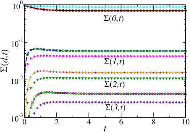
Figure 1: The figure shows the evolution of $\Sigma(x,t)$ for x=0,1,2,3 for a 10 particle system with $r=1/2,~{}r_{w}=1/2$, $\sigma=1$, $\tau_{c}=\tau_{w}=1$. The triangles depict the same system with the constraint that only those pairs with positive relative velocity will collide.

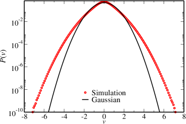
Figure 2: The velocity distribution of a $50$ particle system with $r=1/2,~{}r_{w}=1/2$, $\sigma=1$, $\tau_{c}=1$ and $\tau_{w}=1$. The solid line shows the Gaussian with variance calculated for the system. One can see the deviation from Gaussian.

The steady state values can be obtained by solving Eq. (5) with the left-hand side equated to zero. The elements of $Z_{ss}$, the steady-state correlation vector, $\Sigma_{ss}(x)=\Sigma(x,t\to\infty)$, are obtained from,

$$Z_{ss}={\bf A}^{-1}C.$$ (7)

Here $x\equiv|i-j|$, denotes the separation between lattice points, which takes integer values. Only the first column of the matrix ${\bf A}^{-1}$ suffices to calculate all the elements as,

$$\Sigma_{ss}(x)=A^{-1}_{x0}\sigma^{2}/\tau_{w}.$$ (8)

Calculation of $A^{-1}_{x0}$ is easy due to the tri-diagonal nature of ${\bf A}^{-1}$. The explicit formula for $x=0$ follows as,

$$\begin{split}A^{-1}_{00}=&\frac{a^{n}}{\det{\bf{A}}}\left\{\left[2c-(1-\epsilon)\right]\left[(s^{n-1}+s^{-(n-1)}\right]\right.\\ &\left.-\left[s^{[n-2]}+s^{-[n-2]}\right]\right\},\end{split}$$ (9)

for $x=1,2,..n$:

$$\begin{split}A^{-1}_{x0}&=\frac{\epsilon a^{n}}{\det{\bf{A}}}\left[s^{n-x}+s^{-(n-x)}\right]~{},\end{split}$$ (10)

where

$$c\equiv(1+b/a)~{}~{}\text{and}~{}~{}s\equiv(c+\sqrt{c^{2}-1}).$$ (11)

As $b$ and $a$ takes positive values, $c$ and $s$ will always be greater than or equal to $1$ (equal to $1$ when $r_{w}=-1$). The determinant of the matrix ${\bf{A}}$, denoted as $\det{\bf{A}}$ has the form

$$\begin{split}\det{\bf A}=&a^{n+1}\left\{K_{1}\left[s^{n-1}+s^{-(n-1)}\right]\right.\\ &\left.-K_{2}\left[s^{n-2}+s^{-(n-2)}\right]\right\},\end{split}$$ (12)

where $K_{1},~{}K_{2}$ are functions of ($\epsilon,c,r_{w}$) given by:

$$\begin{split}K_{1}&=2\epsilon+(c-1)[4\epsilon+(1-r_{w})(1+\epsilon)]+2(c-1)^{2}(1-r_{w}),\\ K_{2}&=2\epsilon+(1-r_{w})(c-1).\end{split}$$ (13)

For a large system, one can calculate the asymptotic form of the correlation function $\Sigma_{ss}(x)$. To do this, let us rearrange Eq. (10) to obtain

$$\begin{split}A^{-1}_{x0}&=\frac{\epsilon a^{n}s^{n}}{\det{\bf{A}}}\left[(s^{-x}+s^{-(2n-x)})\right].\end{split}$$ (14)

As $s>1$, in the large $n$ limit the Eq. (14) becomes,

$$A^{-1}_{x0} =\frac{\epsilon a^{n}s^{n}}{\det{\bf{A}}}\left[s^{-x}\right].$$ (15)

Similarly, from Eq. (12), for large $n$, $\det{\bf A}$ can be shown to have the form,

$$\begin{split}\det{\bf A}=a^{(n+1)}s^{n}\left[K_{1}cs^{-1}-K_{2}s^{-2}\right].\end{split}$$ (16)

Thus in large $n$ limit, $\Sigma_{ss}(x)$ has the following form:

$$\Sigma_{d}^{ss}=B\exp(-x\ln s)~{},~{}~{}$$ (17a)

$$B=\frac{\epsilon s}{2(1-\epsilon)(\frac{\tau_{w}}{\tau_{c}})\left(K_{1}-K_{2}\right)}.$$ (17b)

This shows that the system has a finite correlation length $\xi=1/\ln s$. In Fig. 3 we plot the asymptotic form (Eq. (17)) along with the numerical (Eq. (8)) and simulation results. By expanding $\ln s$ near $s=1$, one can see that the correlation length $\xi$ diverges as $1/\sqrt{(1+r_{w})}$ when $r_{w}$ approaches $-1$ from above.

The probability distribution function (PDF) of the velocity at the sites can be obtained from direct simulations. In Fig. 2 the Velocity PDF is plotted as red circles. The non-Maxwellian nature of the PDF is shown by comparing it with a Gaussian (black solid line) function, which has the same variance as that of the PDF.

As indicated before, the above analysis cannot be done for a system with the kinematic constraint. The steady-state correlation $\Sigma_{ss}(x)$ for a system with the constraint is obtained from simulation and is plotted in Fig. 3. The correlation in this case is not the same as that of the model without the constraint. As it is difficult to obtain $\Sigma_{ss}(x)$ for higher $x$ values from simulations, the characteristics of the function are not clear.

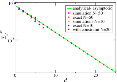
Figure 3: Steady-state values of $\Sigma_{ss}(x)$ for the simulation of $10$ and $50$-particle systems with $r=1/2,~{}r_{w}=1/2$, $\sigma=1$, $\tau_{c}=1$ and $\tau_{w}=1$. The rate of collision is independent of the variance. The exact analytical results, given by Eq. (8), are shown by the ‘$+$’ symbol for $(N=50)$ and ‘$\times$’ for $N=10$. The asymptotic expression Eq. (17) is represented by the solid green line. The triangles show simulation results for the case in which particles collide only when their relative velocity is positive.

V Two-time correlations

By proceeding as in the equal time case in Sec. III, it is easy to obtain the equations of motion for the time-dependent correlation functions defined by $C_{i,j}(t)=\langle v_{i}(t)v_{j}(0)\rangle$, where the average is over the dynamics. The translation invariance of the system means that $C_{ij}(t)=C(i-j,t)$. We get the following equation for $C(x,t)$.

$$\frac{dC(x,t)}{dt}=\left[\frac{a}{2}\Delta_{1}-b\right]C(x,t)~{},$$ (18)

where $\Delta_{1}C(x,t)=C(x+1,t)-2C(x,t)+C(x-1,t)$ . Taking the limit $N\to\infty$ and defining the Fourier transform

$$\widetilde{C}(q,t)=\sum_{x}e^{iqx}C(x,t),$$

we get the following solution

$$\widetilde{C}(q,t)=\exp\left[-(b+a(1-\cos q))t\right]~{}\widetilde{C}(q,t=0)~{},$$ (19)

where

$$\widetilde{C}(q,t=0)=\sum_{x}e^{iqx}C(x,t=0)~{}.$$ (20)

From Eq. (17) we have $C(x,t=0)=B\exp{(-|x|/\xi)}$, which gives

$$\widetilde{C}(q,t=0)=B\frac{s^{2}-1}{s^{2}+1-2s\cos{q}}~{}.$$ (21)

Therefore, the two-time correlation function can be obtained as

$$C(x,t)=\frac{1}{2\pi}\int_{-\pi}^{\pi}\widetilde{C}(q,t)\,e^{-iqx}\,dq=B\,e^{-bt}\,C_{1}(x,t),$$ (22)

where $C_{1}(x,t)$ is given by

$$C_{1}(x=\ell at,t)=\frac{(s^{2}-1)}{2\pi}\int_{-\pi}^{\pi}\frac{\exp\left(-\bigl{[}(1-\cos q)+iq\ell\bigr{]}at\right)}{s^{2}+1-2s\cos{q}}\,dq.$$ (23)

It immediately follows from the above integral that $C_{1}(-x,t)=C_{1}(x,t)$. Therefore, in the following, we consider the case $x\geq 0$. For large $t$, the above integral can be evaluated by saddle point method, which suggests the form

$$C_{1}(x=\ell at,t)\sim e^{-atI(\ell)}.$$ (24)

The saddle point is given by

$$q^{*}=-i\ln\left[\ell+\sqrt{1+\ell^{2}}\right],$$ (25)

which lies on the negative imaginary $q$ axis. However, before proceeding with the saddle-point calculation, we note that the integrand has a simple pole on the negative imaginary $q$ axis at $q_{0}=-i\ln s$ (there is also another one at $+i\ln s$ which do not interfere with the saddle point calculation). Now, for $\ell<(s^{2}-1)/(2s)$ the saddle point lies between the origin and $q_{0}$. Therefore, the contour of integration can be taken through the saddle point without crossing the pole. On the other hand, for $\ell>(s^{2}-1)/(2s)$, the pole lies between the origin and the saddle point. Therefore, in this case the dominant contribution to the integral comes from the pole. Thus the function $I(\ell)$ is given by

$$I(\ell)=\begin{cases}I_{1}(\ell)&\text{for}~{}\ell<\ell^{*}\\ I_{2}(\ell)&\text{for}~{}\ell>\ell^{*}\end{cases}$$ (26)

where $\ell^{*}=(s^{2}-1)/(2s)$, and

$$I_{1}(\ell) =(1-\cos q^{*})+iq^{*}\ell$$ (27)

$$=\left(1-\sqrt{1+\ell^{2}}\right)+\ell\ln\left[\ell+\sqrt{1+\ell^{2}}\right],$$ (28)

and

$$I_{2}(\ell) =(1-\cos q_{0})+iq_{0}\ell$$ (29)

$$=-(b/a)+\ell\ln s,$$ (30)

where we have used the simplification $(s-1)^{2}/(2s)=(b/a)$. It is easy to check that $I(\ell)$ has a second order discontinuity at $\ell=\ell^{*}$, that is, $I_{1}(\ell^{*})=I_{2}(\ell^{*})$ and $I^{\prime}_{1}(\ell^{*})=I^{\prime}_{2}(\ell^{*})$ whereas $I^{\prime\prime}_{1}(\ell^{*})\not=I^{\prime\prime}_{2}(\ell^{*})$. It is interesting to note that, similar discontinuities of the rate function have been found recently in various other contexts Sabhapandit2011 ; Sabhapandit2012 ; Pal2013 ; majumdar2015 . It follows from, Eqs. (22), (24), and (30), that for $|x|>\ell^{*}t$, we have

$$C(x,t)\sim B\,e^{-|x|/\xi}=C(x,t=0).$$ (31)

Therefore, while for $|x|<\ell^{*}t$, the correlation function depends on time, for $|x|>\ell^{*}t$, it still retains the initial form. Such dynamical transition has been found recently in a different context majumdar2015 . The physical reason is that in both of these systems, disturbances take a finite time to propagate from one point to another.

Finally, following the method used in Ref. Sabhapandit2012 , we can also write down a more complete asymptotic form of $C_{1}(x,t)$ for large $t$ as,

$$C_{1}(x=\ell at,t)\approx\frac{e^{-atI_{1}(\ell)}}{\sqrt{2\pi at}} \left[\frac{(s^{2}-1)}{(1+\ell^{2})^{1/4}\,\left(s^{2}+1-2s\sqrt{1+\ell^{2}}\right)}+\frac{\mathrm{sgn}(\ell-\ell^{*})}{\sqrt{2\bigl{[}I_{1}(\ell)-I_{2}(\ell)\bigr{]}}}\right]$$

$$+e^{-atI_{2}(\ell)} \left[\theta(\ell-\ell^{*})-\frac{1}{2}\mathrm{sgn}(\ell-\ell^{*})\,\mathrm{erfc}\sqrt{at\bigl{[}I_{1}(\ell)-I_{2}(\ell)\bigr{]}}\right],$$ (32)

where $I_{1}(\ell)$ and $I_{2}(\ell)$ are given by Eqs. (28) and (30) respectively.

Figure 4 compares the above result with the exact $C_{1}(x,t)$ obtained by numerically integrating Eq. (23) and finds perfect agreement between the two.

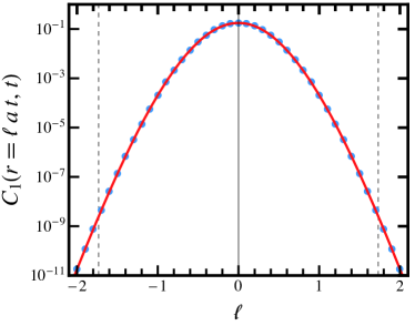
Figure 4: The points are obtained by numerically integrating Eq. (23), whereas the solid line represents the analytical form given by Eq. (32). The parameters used are $\tau_{c}=\tau_{w}=1$, $r=r_{w}=1/2$ and $t=10$. These correspond to $a=b=3/2$ and $s=2+\sqrt{3}$. The vertical dashed lines plot the location of $\pm\ell^{*}$ where $\ell^{*}=\sqrt{3}$.

As a special case, we find for large $t$ the form

$$C(0,t)\approx\frac{B(s+1)e^{-bt}}{(s-1)\sqrt{2\pi at}}.$$ (33)

Thus there is an exponential decay as a function of time with a $1/\sqrt{t}$ prefactor.

VI Conclusion

In this work, we studied a simple model for driven inelastic gas in one dimension for which we find the equal-time spatial velocity correlation functions as well as two-time correlation functions in the steady state. The equal-time correlations decay exponentially in space. An interesting finding is that there exists a velocity $l^{*}a$ such that the decay of correlations does not propagate beyond a distance $|x|=l^{*}at$, which leads to second order dynamical transition in the spatio-temporal correlation function. Such transitions have never been discussed in the context of granular physics, and therefore, this study opens up a new direction of research in granular physics. Hopefully, in future experiments, such transitions could be observed in real granular systems.

We also obtain the condition for the existence of a steady state for the model. Experimental studies on granular gases driven by wall collisions, have found an exponential decay for the spatial correlation functions of velocity Prevost:02 ; Gradenigo:11 . Simple but exact models such as the one introduced here may facilitate a better understanding of the observed features. It will be interesting to study the nature of correlations in other models of granular systems with different interactions and driving mechanisms.

Appendix A BBGKY hierarchy

Here we show that the equations for the correlations Eq. (3) can also be derived by starting from the BBGKY hierarchy for the distribution functions. Let $P_{1}(v_{i},t)$ be the 1-point probability distribution function for the site $i$ to have the velocity variable $v_{i}$ at time $t$. Similarly $P_{2}(v_{i},v_{i+x},t)$ be the 2-site probability distribution function for the sites $i,~{}i+x$ to have velocities $v_{i},~{}v_{i+x}$ at time $t$. Similarly defined is the 3-site probability distribution function $P_{3}(v_{i-m},v_{i},v_{i+x})$ ($\{m,x\}$ are integers less than $N$). For the dynamics in Eqs. (1,2), one can immediately write a set of evolution equation for the distributions as,

$$\frac{\partial}{\partial t}P_{1}(v_{i},t)=\tau_{c}^{-1}\left[\int dv_{i+1}\overline{T}(v_{i},v_{i+1})P_{2}(v_{i},v_{i+1},t)+\overline{T}(v_{i-1},v_{i})P_{2}(v_{i-1},v_{i},t)\right]\hskip 199.16928pt$$

$$+\tau_{w}^{-1}\left[\int dv_{i}^{*}P_{1}(v_{i}^{*},t)\langle\delta\left(v_{i}-[-r_{w}v_{i}^{*}+\eta_{i}]\right)\rangle_{\eta_{i}}-P_{1}(v_{i},t)\right],\hskip 199.16928pt$$ (34a)

$$\frac{\partial}{\partial t}P_{2}(v_{i},v_{i+x},t)=\tau_{c}^{-1}\left\{\overline{T}(v_{i},v_{i+x})P_{2}(v_{i},v_{i+x},t)\delta_{x,1}+\int dv_{i-1}\overline{T}(v_{i-1},v_{i})P_{3}(v_{i-1},v_{i},v_{i+x},t)+\right.\hskip 190.63338pt$$

$$\left.\left[\int dv_{i+1}\overline{T}(v_{i},v_{i+1})P_{3}(v_{i},v_{i+1},v_{i+x},t)+\int dv_{i+x-1}\overline{T}(v_{i+x-1},v_{i+x})P_{3}(v_{i},v_{i+x-1},v_{i+x},t)\right](1-\delta_{x,1})+\hskip 71.13188pt\right.$$

$$\int dv_{i+x+1}\overline{T}(v_{i+x},v_{i+x+1})P_{3}(v_{i},v_{i+x},v_{i+x+1},t)\bigg{\}}\hskip 284.52756pt$$

$$\quad+\tau_{w}^{-1}\left[\int dv_{i}^{*}P_{2}(v^{*}_{i},v_{i+x},t)\langle\delta\left(v_{i}-[-r_{w}v^{*}_{i}+\eta_{i}]\right)\rangle_{\eta_{i}}+\right.\hskip 273.14662pt$$

$$\left.\int dv_{i+x}^{*}P_{2}(v_{i},v^{*}_{i+x},t)\langle\delta\left(v_{i+x}-[-r_{w}v_{i+x}^{*}+\eta_{i+x}]\right)\rangle_{\eta_{i+x}}-2P_{2}(v_{i},v_{i+x},t)\right].\hskip 190.63338pt$$ (34b)

and so on. Here, $\overline{T}(v_{i},v_{j})$ defined as, $\overline{T}(v_{i},v_{j})S(v_{i},v_{j})=r^{-1}S(v_{i}^{*},v_{j}^{*})-S(v_{i},v_{j})$, and acts only on the two variables designated by the arguments of the $\overline{T}$ operator. Also $\delta_{i,j}$ is the Kronecker delta function. The evolution of the distribution functions thus involves a hierarchy of equations. The solution would require a closure of this hierarchy. As for the Maxwell particles Prasad:14 , one may ask whether there exists such a closure in terms of the variance and two-point correlation functions for the one-dimensional lattice gas also.

We calculate the evolution of the function $\Sigma(x,t)$, by multiplying $v_{i}v_{i+x}$ and integrating over $v_{i}$ and $v_{i+x}$. This results in the closed set of equations for $\Sigma$ given in Eq. (3).

Appendix B Existence of steady states for various values of $r_{w}$ for the inelastic gas on a 1-D lattice

B.1 Absence of steady state when $r_{w}=-1$

Here, we show that the correlation vector $Z(t)$ which evolves according to Eq. (5), does not have a steady state when $r_{w}=-1$. To show this, we observe the properties of the eigenvalues of the matrix $\bf A$ (Eq. (6)). We note that when $r_{w}=-1$, the parameter $b$ is equal to zero and the tri-diagonal matrix ${\bf A}$ has a simpler form (Eq. (35)). We denote this matrix by ${\bf A}({r_{w}=-1})$.

$${\footnotesize{\bf{A}}({r_{w}=-1}})=\;{\mathnormal{a^{n+1}}}\;{\footnotesize\begin{bmatrix}2\epsilon&-2\epsilon&&&&&&\\ -\epsilon&(1+\epsilon)&-1&&&\mbox{\Huge 0}&&\\ &-1&2&-1&&&&\\ &&\ddots&\ddots&\ddots&&&\\ &\mbox{\Huge{{0}}}&&&-1&2&-1&\\ &&&&&-2&2\end{bmatrix}}.$$ (35)

The determinant of the above $(n+1)$-th order matrix denoted as $\det{\bf A}({r_{w}=-1})$, can be shown to satisfy the relation, when $n>2$:

$$\det{\bf A}({r_{w}=-1})=2\epsilon a^{n+1}\left[\det{\bf A}^{\prime}_{n-1}-~{}\det{\bf A}^{\prime}_{n-2}\right],$$ (36)

where $\det{\bf A}^{\prime}_{k}$ is the determinant of ${\bf A}^{\prime}_{k}$, which is a matrix of order $k\in\mathbb{N}$, and has the form given below.

$$\bf{A}^{\prime}=\begin{bmatrix}2&-1&&&&&&\\ -1&2&-1&&&\mbox{\Huge 0}&&\\ &-1&2&-1&&&&\\ &&\ddots&\ddots&\ddots&&&\\ &\mbox{\Huge{{0}}}&&&-1&2&-1&\\ &&&&&-2&2\end{bmatrix}$$ (37)

One can find $\det\bf{A}^{\prime}_{k}$, as follows. Let us denote $\det{\bf{A}}^{\prime}_{k}\equiv D^{\prime}_{k}$. It can be shown to satisfy the relation,

$$D^{\prime}_{k}-2D^{\prime}_{k-1}+D^{\prime}_{k-2}=0.$$ (38)

Using the boundary conditions, $D^{\prime}_{1}=2$, $D^{\prime}_{2}=2$, the solution of Eq. (38) can be easily obtained as, $D^{\prime}_{k}=\det{\bf{A}}^{\prime}_{k}=2$. Substituting this in Eq. (36) we obtain the result, $\det{\bf A}({r_{w}=-1})=0$. This shows that at least one of the eigenvalue is zero, which implies the lack of steady state for the system.

B.2 Presence of steady state when $|r_{w}|<1$

Consider the matrix ${\bf A}$ (Eq. (6)) when $r_{w}\not=-1$. We can use Gershgorin circle theorem bell:65 to predict the range of the eigenvalues of the matrix ${\bf A}$. The theorem states that any eigenvalue $\lambda$ of the matrix ${\bf A}$ should satisfy the condition:

$$|\lambda-{\bf A}_{ii}|\leq\displaystyle\sum\limits_{j\neq i}|{\bf A}_{ij}|~{}~{},i=0,1,2...n$$ (39)

From the first row of ${\bf A}$, we find that:

$$|\lambda-\left[2\epsilon a+b(1-r_{w})\right]|\leq 2\epsilon a,$$ (40)

which says, $\lambda-b(1-r_{w})\geq 0$. Similarly for $i>1$, using Eq. (39) we obtain the result, $\lambda-2b\geq 0$. Thus all the eigenvalues are strictly greater than zero as $b>0$. This proves that when $|r_{w}|<1$, the system goes to a steady state.

B.3 Presence of steady state when $r_{w}=1$

When $r_{w}=1$, Gershgorin circle theorem provides the inequalities, $\lambda\geq 0$ from the first row of ${\bf A}({r_{w}=1})$ and $\lambda-2b\geq 0$ from other rows of ${\bf A}({r_{w}=1})$, to be satisfied by the eigenvalues $\lambda$ of ${\bf A}({r_{w}=1})$. The above observations show that the eigenvalues of ${\bf A}({r_{w}=1})$ will satisfy the condition $\lambda\geq 0$. But if the system goes to a steady state, the eigenvalues should be strictly positive. This is true if the determinant, $\det{\bf A}({r_{w}=1})\neq 0$. We show this in the following.

As we are interested in the large system case, we consider a system with $n>2$. For the system, one can show as before, that $\det{\bf A}({r_{w}=1})$ satisfies the equation,

$$\det{\bf A}({r_{w}=1})=2\epsilon a^{n+1}\left[(2c-1)~{}\det{\bf A}^{{}^{\prime\prime}}_{n-1}-\det{\bf A}^{{}^{\prime\prime}}_{n-2}\right],$$ (41)

where ${\bf A}^{{}^{\prime\prime}}_{k}$ is a $k\times k$ matrix given by,

$$\bf{A}^{{}^{\prime\prime}}_{k}=\begin{bmatrix}2c&-1&&&&&&\\ -1&2c&-1&&&\mbox{\Huge 0}&&\\ &-1&2c&-1&&&&\\ &&\ddots&\ddots&\ddots&&&\\ &\mbox{\Huge{{0}}}&&&-1&2c&-1&\\ &&&&&-2&2c\end{bmatrix}.$$ (42)

We define the determinant, $\det{\bf A}^{{}^{\prime\prime}}_{k}\equiv D^{{}^{\prime\prime}}_{k}$. From Eq. (42), one can show that $D^{{}^{\prime\prime}}_{k}$ satisfies the equation,

$$D^{{}^{\prime\prime}}_{k}-2cD^{{}^{\prime\prime}}_{k-1}+D^{{}^{\prime\prime}}_{k-2}=0,~{}k=3,4..$$ (43)

with $c=1+b/a$. The exact form of $D^{{}^{\prime\prime}}_{k}$ can be found by solving the difference equation using the initial conditions $D^{{}^{\prime\prime}}_{1}=2c$, $D^{{}^{\prime\prime}}_{2}=4c^{2}-2$. The general solution for Eq. (43) has the form,

$$D^{{}^{\prime\prime}}_{k}=As^{k}+Bs^{-k},$$ (44)

with $s=c+\sqrt{c^{2}-1}$. Using the initial conditions, the exact form of $D^{{}^{\prime\prime}}_{k}$ is found as,

$$D^{{}^{\prime\prime}}_{k}=s^{k}+s^{-k}.$$ (45)

Substituting $\det{\bf A}^{{}^{\prime\prime}}_{k}=(s^{k}+s^{-k})$ in Eq. (41), one gets:

$$\det{\bf A}({r_{w}=1})= 2\epsilon a^{(n+1)}\left((1+2b/a)\left[s^{(n-1)}+s^{-(n-1)}\right]\right.$$ (46)

$$\left.-\left[s^{(n-2)}+s^{-(n-2)}\right]\right).$$

One can rewrite the Eq. (46) as,

$$\det{\bf A}({r_{w}=1})= 2\epsilon a^{(n+1)}\times\big{\{}\left[s^{(n-1)}-s^{(n-2)}\right.$$

$$\left.+s^{-(n-1)}-s^{-(n-2)}\right] +\frac{2b}{a}\left[s^{(n-1)}+s^{-(n-1)}\right]\big{\}}.$$ (47)

Note that $s>1$. The material within the first set of square brackets on the right-hand side of Eq. (47) can be rewritten as,

$$\left[s^{(n-1)}-s^{(n-2)}+\frac{1}{s^{(n-1)}}-\frac{1}{s^{(n-2)}}\right]=\left(s^{2n-3}-1\right)\frac{s-1}{s^{n-1}}>0\hskip 28.45274pt$$ (48)

for $s>1$ and $n\geq 2$. As the term in the second set of square brackets in Eq. (47) is a positive definite quantity, the right-hand side of Eq. (47) will be non-zero. So the determinant of ${\bf A}({r_{w}=1})$ is non-zero.

References

- (1) P. L. Garrido, J. L. Lebowitz, C. Maes, H. Spohn, Phys. Rev. A 42, 1954 (1990).
- (2) T. P. C. van Noije and M. H. Ernst, Granular Matter 1, 57 (1998).
- (3) F. Rouyer and N. Menon Phys. Rev. Lett. 85, 3676 (2000).
- (4) E. Ben-Naim and P. L. Krapivsky, Phys. Rev. E 61, R5 (2000).
- (5) A. Santos and M. H. Ernst, Phys. Rev. E 68, 011305 (2003).
- (6) J. S. van Zon and F. C. MacKintosh Phys. Rev. Lett. 93, 038001 (2004).
- (7) E. Ben-Naim and J. Machta, Phys. Rev. Lett. 94, 138001 (2005).
- (8) V. V. Prasad, S. Sabhapandit, and A. Dhar, Europhys. Lett., 104, 54003 (2013) .
- (9) T. P. C. van Noije, M. H. Ernst, R. Brito and, J. A. G. Orza, Phys. Rev. Lett. 79, 411 (1997).
- (10) A. Baldassarri , U. Marini Bettolo Marconi, and A. Puglisi, Europhys. Lett., 58,14 (2002).
- (11) M. Shinde, D. Das, and R. Rajesh Phys. Rev. Lett. 99, 234505 (2007).
- (12) J. Javier Brey and M. J. Ruiz-Montero, Phys. Rev. E 91, 012202 (2015).
- (13) D. R. M. Williams and F. C. MacKintosh, Phys. Rev. E 54, R9(R) (1996).
- (14) S. J. Moon, M. D. Shattuck, and J. B. Swift Phys. Rev. E 64, 031303 (2001).
- (15) M. R. Swift, M. Boamfa, S. J. Cornell, and A. Maritan, Phys. Rev. Lett. 80, 4410 (1998)
- (16) T. P. C. van Noije, M. H. Ernst, E. Trizac, and I. Pagonabarraga, Phys. Rev. E 59, 4326 (1999).
- (17) D. L. Blair and A. Kudrolli, Phys. Rev. E 64, 050301(R) (2001).
- (18) A. Prevost, D. A. Egolf, and J. S. Urbach, Phys. Rev. Lett. 89, 084301 (2002).
- (19) G. Gradenigo, A. Sarracino, D. Villamaina and A. Puglisi, Europhys. Lett. 96 14004 (2011); A. Puglisi, A. Gnoli , G. Gradenigo, A. Sarracino and D. Villamaina, J. Chem. Phys. 136, 014704 (2012).
- (20) A. Lasanta, A. Manacorda, A. Prados and A. Puglisi, New J. Phys. 17 083039 (2015).
- (21) C. A. Plata, A. Manacorda, A. Lasanta, A. Puglisi, A. Prados, J. Stat. Mech.: Theory Exp., (2016) 093203.
- (22) A. Manacorda, C. A. Plata, A. Lasanta, A. Puglisi, A. Prados, J. Stat. Phys. 164 810 (2016).
- (23) V. V. Prasad, S. Sabhapandit, and A. Dhar, Phys. Rev. E 90, 062130 (2014).
- (24) D. Levanony and D. Levine, Phys. Rev. E 73, 055102R (2006).
- (25) A. Prados, A. Lasanta, and P. I. Hurtado, Phys. Rev. Lett. 107, 140601, (2011).
- (26) A. Prados, A. Lasanta, and P. I. Hurtado Phys. Rev. E 86, 031134 (2012).
- (27) P. I. Hurtado, A. Lasanta, and A. Prados, Phys. Rev. E 88, 022110 (2013).
- (28) P. Maynar, M. de Soria, and E. Trizac, Eur. Phys. J. Spec. Top. 179, 123 (2009).
- (29) V. Privman, Nonequilibrium Statistical Mechanics in One Dimension (Cambridge University Press, 1997).
- (30) A. Baldassarri, U. Marini Bettolo Marconi, and A. Puglisi Phys. Rev. E 65, 051301 (2002).
- (31) S. Sabhapandit, Europhys. Lett. 96, 20005 (2011).
- (32) S. Sabhapandit, Phys. Rev. E 85, 021108 (2012).
- (33) A. Pal and S. Sabhapandit, Phys. Rev. E 87, 022138 (2013).
- (34) S. N. Majumdar, S. Sabhapandit, and G. Schehr, Phys. Rev. E 91, 052131 (2015); 92, 052126 (2015).
- (35) H. E. Bell, The American Mathematical Monthly 72, 292 (1965).