Neural Network-based Word Alignment through Score Aggregation

Abstract

We present a simple neural network for word alignment that builds source and target word window representations to compute alignment scores for sentence pairs. To enable unsupervised training, we use an aggregation operation that summarizes the alignment scores for a given target word. A soft-margin objective increases scores for true target words while decreasing scores for target words that are not present. Compared to the popular Fast Align model, our approach improves alignment accuracy by 7 AER on English-Czech, by 6 AER on Romanian-English and by 1.7 AER on English-French alignment.

1 Introduction

Word alignment is the task of finding the correspondence between source and target words in a pair of sentences that are translations of each other. Generative models for this task (Brown et al., 1990; Och and Ney, 2003; Vogel et al., 1996) still form the basis for many machine translation systems (Koehn et al., 2003; Chiang, 2007).

Recent neural approaches include Yang et al. (2013) who introduce a feed-forward network-based model trained on alignments that were generated by a traditional generative model. This treats potentially erroneous alignments as supervision. Tamura et al. (2014) sidesteps this issue by negative sampling to train a recurrent-neural network on unlabeled data. They optimize a global loss that requires an expensive beam search to approximate the sum over all alignments.

In this paper we introduce a word alignment model that is simpler in structure and which relies on a more tractable training procedure. Our model is a neural network that extracts context information from source and target sentences and then computes simple dot products to estimate alignment links. Our objective function is word-factored and does not require the expensive computation associated with global loss functions. The model can be easily trained on unlabeled data via a novel but simple aggregation operation which has been successfully applied in the computer vision literature (Pinheiro and Collobert, 2015). The aggregation combines the scores of all source words for a particular target word and promotes source words which are likely to be aligned with a given target word according to the knowledge the model has learned so far. At test time, the aggregation operation is removed and source words are aligned to target words by choosing the highest scoring candidates (§2, §3).

We evaluate several forms for our aggregation operation such as computing the sum, max and LogSumExp over alignment scores. Results on English-French, English-Romanian, and Czech-English alignment show that our model significantly outperforms Fast Align, a popular log-linear reparameterization of IBM Model 2 (Dyer et al., 2013; §4).

2 Aggregation Model

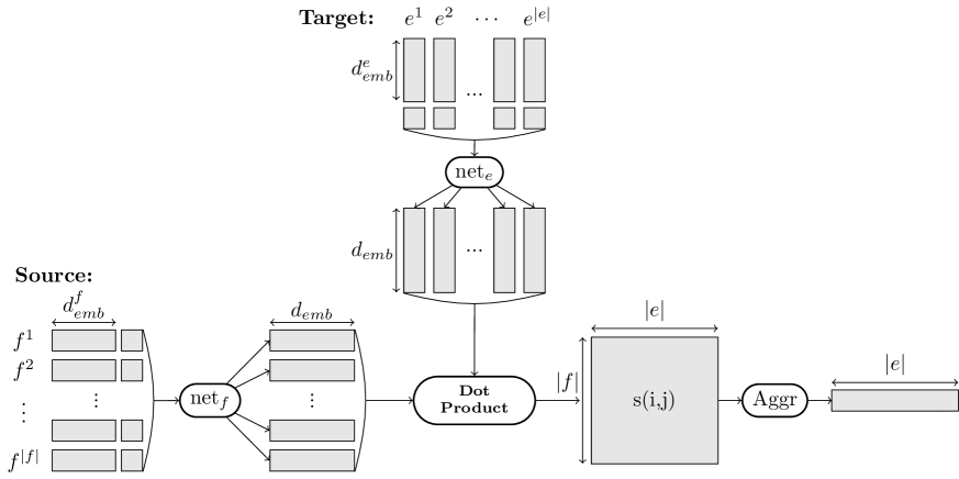
Figure 1: Illustration of the model. The two networks $\textrm{net}_{e}$ and $\textrm{net}_{f}$ compute representations for source and target words. The score of an alignment link is a simple dot product between those source and target word representations. The aggregation operation summarizes the alignment scores for each target word.

In the following, we consider a target-source sentence pair $(\mathbf{e},\,\mathbf{f})$, with $\mathbf{e}=(e_{1},\,\dots,\,e_{|\mathbf{e}|})$ and $\mathbf{f}=(f_{1},\,\dots,\,f_{|\mathbf{f}|})$. Words are represented by $f_{j}$ and $e_{i}$, which are indices in source and target dictionaries. For simplicity, we assume here that word indices are the only feature fed to our architecture. Given a source word $f_{j}$ and a target word $e_{i}$, our architecture embeds a window (of size $d^{f}_{win}$ and $d^{e}_{win}$, respectively) centered around each of these words into a $d_{emb}$-dimensional vector space. The embedding operation is performed with two distinct neural networks:

$$\textrm{net}_{e}(\left[\mathbf{e}\right]_{i}^{d^{e}_{win}})\in\mathbb{R}^{d_{emb}}$$

and

$$\textrm{net}_{f}(\left[\mathbf{f}\right]_{j}^{d^{f}_{win}})\in\mathbb{R}^{d_{emb}}\,,$$

where we denote the window operator as

$$\left[\mathbf{x}\right]_{i}^{d}=(x_{i-d/2},\dots,x_{i+d/2})\,.$$

The matching score between a source word $f_{j}$ and a target word $e_{i}$ is then given by the dot-product:

$$s(i,\,j)=\textrm{net}_{e}(\left[\mathbf{e}\right]_{i}^{d^{e}_{win}})\cdot\textrm{net}_{f}(\left[\mathbf{f}\right]_{j}^{d^{f}_{win}})\,.$$ (1)

If $e_{i}$ is aligned to $f_{a_{i}}$, the score $s(i,\,a_{i})$ should be high, while scores $s(i,\,j)\ \forall j\neq a_{i}$ should be low.

2.1 Unsupervised Training

In this paper, we consider an unsupervised setup where the alignment is not known at training time. We thus cannot minimize or maximize matching scores (1) in a direct manner. Instead, given a target word $e_{i}$ we consider the aggregated matching scores over the source sentence:

$$s_{aggr}(i,\mathbf{f})=\operatorname*{Aggr}_{j=1}^{|\mathbf{f}|}s(i,\,j)\,,$$ (2)

where $\operatorname*{Aggr}$ is an aggregation operator (§2.2). Consider a matching (positive) sentence pair $(\mathbf{e}^{+},\mathbf{f})$ and a negative sentence pair $(\mathbf{e^{-}},\mathbf{f})$. Given a word at index $i^{+}$ in the positive target sentence, we want to maximize the aggregated score $s_{aggr}(i^{+},\mathbf{f})$ ($1\leq i^{+}\leq|\mathbf{e^{+}}|$) because we know it should be aligned to at least one source word. Conversely, given a word at index $i^{-}$ in the negative target sentence, we want to minimize $s_{aggr}(i^{-},\mathbf{f})$ ($1\leq i^{-}\leq|\mathbf{e^{-}}|$) because it is unlikely that the source sentence can explain the negative target word. Following these principles, we consider a simple soft-margin loss:

$${\cal L}(\mathbf{e}^{+},\,\mathbf{e}^{-},\,\mathbf{f}) =\sum_{i^{+}=1}^{|\mathbf{e^{+}}|}\log(1+e^{-s_{aggr}(i^{+},\mathbf{f})})$$

$$+\sum_{i^{-}=1}^{|\mathbf{e^{-}}|}\log(1+e^{+s_{aggr}(i^{-},\mathbf{f})})\,.$$ (3)

Training is achieved by minimizing (3) and by sampling over triplets $(\mathbf{e}^{+},\,\mathbf{e}^{-},\,\mathbf{f})$ from the training data.

2.2 Choosing the Aggregation

The aggregation operation (2) is only present during training and acts as a filter which aims to explain a given target word $e_{i}$ by one or more source words. If we had the word alignments, then we would sum over the source words $f_{j}$ aligned with $e_{i}$. However, in our setup alignments are not available at training time, so we must rely on what the model has learned so far to filter the source words. We consider the following strategies:

• Sum: ignore the knowledge learned so far, and assign the same weight to all source words $f_{j}$ to explain $e_{i}$. In this case, we have

  $$s_{aggr}(i,\mathbf{f})=\sum_{j=1}^{|\textbf{f}|}s(i,\,j)\,.$$

• Max: encourage the best aligned source word $f_{j}$, according to what the model has learned so far. In this case, the aggregation is written as:

  $$s_{aggr}(i,\mathbf{f})=\max_{j=1}^{|\textbf{f}|}s(i,\,j)\,.$$

• LSE: give similar weights to source words with similar scores. This can be achieved with a LogSumExp aggregation operation (also called LogAdd), and is defined as:

  $$s_{aggr}(i,\mathbf{f})=\frac{1}{r}\log\left(\sum_{j=1}^{|\textbf{f}|}e^{r\,s(i,\,j)}\right)\,,$$ (4)

  where $r$ is a positive scalar (to be chosen) controlling the smoothness of the aggregation. For small $r$, the aggregation is equivalent to a sum, and for large $r$, the aggregation acts as a max.

2.3 Decoding

At test time, we align each target word $e_{i}$ with the source word $f_{j}$ for which the matching score $s(i,\,j)$ in (1) is highest. However, not every target word is aligned, so we consider only alignments with a matching score above a threshold:

$$s(i,\,j)>\mu^{-}(e_{i})+\alpha\,\sigma^{-}(e_{i})\,,$$ (5)

where $\alpha$ is a tunable hyper-parameter, and

$$\mu^{-}(e_{i})=\mathop{{}\mathbb{E}}_{\{\tilde{e}_{k}=e_{i}\,\in\,\mathbf{\tilde{e}},\,\tilde{f}_{j^{-}}\,\in\,\mathbf{\tilde{f}-}\}}\left[s(k,\,j^{-})\right]$$

is the expectation over all training sentences $\tilde{\mathbf{e}}$ containing the word $e_{i}$, and all words $\tilde{f}^{-}_{j}$ belonging to a corresponding negative source sentence $\mathbf{\tilde{f}}^{-}$, and $\sigma^{-}(e_{i})$ is the respective variance.

3 Neural Network Architecture

Our model consists of two convolutional neural networks $\textrm{net}_{e}$ and $\textrm{net}_{f}$ as shown in (1). Both of them take the same form, so we detail only the target architecture.

3.1 Word embeddings

The discrete features $\left[\mathbf{e}\right]_{i}^{d^{e}_{win}}$ are embedded into a $d^{e}_{emb}$-dimensional vector space via a lookup-table operation as first introduced in Bengio et al. (2000):

$$x_{i}^{e} =\textsc{LT}_{W^{e}}(\left[\mathbf{e}\right]_{i}^{d^{e}_{win}})$$

$$=(\textsc{LT}_{W^{e}}(e_{i-d^{e}_{win}/2}),\,\dots,\,\textsc{LT}_{W^{e}}(e_{i+d^{e}_{win}/2}))\,,$$

where the lookup-table operation applied at index $k$ returns the $k^{th}$ column of the parameter matrix $W^{e}$:

$$\textsc{LT}_{W^{e}}(k)=W^{e}_{\bullet,\,k}\,.$$

The matrix $W^{e}$ is of size $|{\cal V}^{e}|\times d^{e}_{emb}$, where ${\cal V}^{e}$ is the target vocabulary, and $d_{emb}^{e}$ is the word embedding size for the target words.

3.2 Convolutional layers

The word embeddings output by the lookup-table are concatenated and fed through two successive 1-D convolution layers. The convolutions use a step size of one and extract context features for each word. The kernel sizes $k_{1}^{e}$ and $k_{2}^{e}$ determine the size of the window $d^{e}_{win}=k_{1}^{e}+k_{2}^{e}-1$ over which features will be extracted by $\textrm{net}_{e}$. In order to obtain windows centered around each word, we add $(k_{1}^{e}+k_{2}^{e})/2-1$ padding words at the beginning and at the end of each sentence.

The first layer $cnn^{e}$ applies the linear transformation $M^{e,1}$ exactly $k_{2}^{e}$ times to consecutive spans of size $k_{1}^{e}$ to the $d^{e}_{win}$ words in a given window:

$$cnn^{e}(x_{i}^{e})=M^{e,1}\begin{pmatrix}\textsc{LT}_{W^{e}}(\left[\mathbf{e}\right]^{k_{1}^{e}}_{i-a})\\ {\vdots}\\ \textsc{LT}_{W^{e}}(\left[\mathbf{e}\right]^{k_{1}^{e}}_{i+a})\\ \end{pmatrix},$$

where $a=\lfloor\frac{k^{e}_{2}}{2}\rfloor$, $M^{e,1}\in\mathbb{R}^{d^{e}_{hu}\times(d^{e}_{emb}\,k^{e}_{1})}$ is a matrix of parameters, and $d^{e}_{hu}$ is the number of hidden units ($hu$). The outputs of the first layer $cnn^{e}$ are concatenated to form a matrix of size $k^{e}_{2}\textrm{ }d^{e}_{hu}$ which is fed to the second layer:

$$\textrm{net}_{e}(x_{i}^{e})=M^{e,2}\,\tanh(cnn^{e}(x_{i}^{e}))\,$$ (6)

where $M^{e,2}\in\mathbb{R}^{d_{emb}\times(k^{e}_{2}~{}d^{e}_{hu})}$ is a matrix of parameters, and the $tanh(\cdot)$ operation is applied element wise. The parameters $W^{e}$, $M^{e,1}$ and $M^{e,2}$ are trained by stochastic gradient descent to minimize the loss (3) introduced in §2.1.

3.3 Additional Features

In addition to the raw word indices, we consider two additional discrete features which were handled in the same way as word features by introducing an additional lookup-table for each of them. The output of all lookup-tables was concatenated, and fed to the two-layer neural network architecture (6).

Distance to the diagonal.

This feature can be computed for a target word $e_{i}$ and a source word $f_{j}$:

$$diag(i,j)=\left|\frac{i}{|\mathbf{e}|}-\frac{j}{|\mathbf{f}|}\right|\,,$$

This feature allows the model to learn that aligned sentence pairs use roughly the same word order and that alignment links remain close to the diagonal. We use this feature only for the source network because it encodes relative position information which only needs to be encoded once. If we would use absolute position instead, then we would need to encode this information both on the source and the target side.

Part-of-speech

Words pairs that are good translations of each other are likely to carry the same part of speech in both languages (Melamed, 1995). We therefore add the part-of-speech information to the model.

Char n-gram.

We consider unigram character position features. Let $K$ be the maximum size for a word in a dictionary. We denote the dictionary of characters as $\mathcal{C}$. Every character is represented by its index $c$ (with $1<c<|\mathcal{C}|$). We associate every character $c$ at position $k$ with a vector at position $((k-1)*|\mathcal{C}|)+c$ in a lookup-table. For a given word, we extract all unigram character position embeddings, and average them to obtain a character embedding for a given word.

4 Experiments

4.1 Datasets

We use the English-French Hansards corpus as distributed by the NAACL 2003 shared task (Mihalcea and Pedersen, 2003). This dataset contains 1.1M sentence pairs and the test and validation sets contain 447 and 37 examples respectively. We also evaluate on the Romanian-English dataset of the ACL 2005 shared task (Martin et al., 2005) comprising 48K sentence pairs for training, 248 for testing and 17 for validation. For English-Czech experiments, we use the WMT news commentary corpus for training (150K sentence pairs) and a set of 515 sentences for testing (Bojar and Prokopová, 2006).

4.2 Evaluation

Our models are evaluated in terms of precision, recall, F-measure and Alignment Error Rate (AER). We train models in each language direction and then symmetrize the resulting alignments using either the intersection or the grow-diag-final-and heuristic (Och and Ney, 2003; Koehn et al., 2003). We validated the choice of symmetrization heuristic on each language pair and chose the best one for each model considering the two aforementioned types as well as grow-diag-final and grow-diag.

Additionally, we train phrase-based machine translation models with our alignments using the popular Moses toolkit (Koehn et al., 2007). For English-French, we train on the news commentary corpus v10, for English-Czech we used news commentary corpus v11, and for Romanian-English we used the Europarl corpus v8. We tuned our models on the WMT2015 test set for English-Czech as well as for Romanian-English; for English-French we tuned on the WMT2014 test set. Final results are reported on the WMT2016 test set for English-Czech as well as Romanian-English, and for English-French we report results on the WMT2015 test set (as there is no track for this language-pair in 2016).

We compare our model to Fast Align, a popular log-linear reparameterization of IBM Model 2 (Dyer et al., 2013).

4.3 Setup

The kernel sizes of the target network $\textrm{net}_{e}(\cdot)$ are set to $k^{e}_{1}=k^{e}_{2}=3$ for all language pairs. The kernel sizes of the source network $\textrm{net}_{f}(\cdot)$ are set to $k^{f}_{1}=k^{f}_{2}=3$ for Romanian-English as well as English-Czech; and for English-French we used $k^{f}_{1}=k^{f}_{2}=1$.

The number of hidden units are $d^{e}_{hu}=d^{f}_{hu}=256$ and $d_{emb}$ is set to 256, The source ${\cal V}_{f}$ and target ${\cal V}_{e}$ dictionaries consist of the 30K most common words for English, French and Romanian, and 80K for Czech. All other words are mapped to a unique UNK token. The word embedding sizes $d^{e}_{emb}$ and $d^{f}_{emb}$, as well as the char-n-gram embedding size is $128$. For LSE, we set $r=1$ in (4).

We initialize the word embeddings with a simple PCA computed over the matrix of word co-occurrence counts (Lebret and Collobert, 2014). The co-occurrence counts were computed over the common crawl corpus provided by WMT16. For part of speech tagging we used the Stanford parser on English-French data, and MarMoT (Mueller et al., 2013) for Romanian-English as well as English-Czech.

We trained 4 systems for the ensembles, each using a different random seed to vary the weight initialization as well as the shuffling of the training set. We averaged the alignment scores predicted by each system before decoding. The alignment threshold variables $\mu^{-}(e_{i})$ and $\sigma^{-}(e_{i})$ for decoding (§2.3) were estimated on 1000 random training sentences, using 100 negative sentences for each of them. Words not appearing in this training subset were assigned $\mu^{-}(e_{i})=\sigma^{-}(e_{i})=0$.

For systems where $d^{e}_{win}>1$ and $d^{f}_{win}>1$, we saw a tendency of aligning frequent words regardless on if they appeared in the center of the context window or not. For instance, a common mistake would be to align ”the cat sat”, with ”PADDING le chat”. To prevent such behavior, we occasionally replaced the center word in a target window by a random word during training. We do this for every second training example on average and we tuned this rate on the validation set.

4.4 Results

We first explore different choices for the aggregation operator (§2.2), followed by an ablation to investigate the impact of the different additional features (§3.3). Next we compare to the Fast Align baseline. Finally, we evaluate our alignments within a full translation system for all language pairs.

4.4.1 Aggregation operation

Table 1 shows that the LogSumExp (LSE) aggregator performs best on all datasets for every direction as well as in the symmetrized setting using the grow-diag-final heuristic. All results are based on a single model trained with the ’distance to the diagonal’ feature detailed above. We therefore use LSE for the remaining experiments.

	Max	Sum	LSE
En-Fr	18.1	23.0	15.1
Fr-En	20.7	26.9	15.8
symmetrized	14.8	24.1	12.8
Ro-En	42.2	42.0	37.6
En-Ro	40.4	40.2	35.7
symmetrized	36.4	35.6	32.2
En-Cz	27.9	35.6	24.5
Cz-En	26.5	33.6	24.5
symmetrized	21.8	32.7	21.0

Table 1: Alignment error rates for different aggregation operations in each language direction and with grow-diag-final-and symmetrization.

4.4.2 Additional features

Table 2 shows the effect of the different input features. Both POS and the distance to the diagonal feature significantly improve accuracy. Position information via the ’distance to the diagonal’ feature is helpful for all language pairs, and POS information is more effective for Romanian-English and English-Czech which involve morphologically rich languages. We use the POS and ’distance to the diagonal feature’ for the remaining experiments.

	English-French			Romanian-English			English-Czech
	En-Fr	Fr-En	sym	Ro-En	En-Ro	sym	En-Cz	Cz-En	sym
words	22.2	24.2	15.7	47.0	45.5	40.3	36.9	36.3	29.5
+ POS	20.9	23.9	15.3	45.3	42.9	36.9	35.6	33.7	28.2
+ diag	15.1	15.8	12.8	37.6	35.7	32.2	24.8	24.5	21.0
+ POS + diag	13.2	12.1	10.2	33.1	32.2	27.8	24.6	22.9	19.9

Table 2: Alignment error rates using different input features in each language direction and with grow-diag-final-and symmetrization.

4.4.3 Comparison with the baseline

In the following results we label our model as NNSA (Neural network score aggregation). On English-French data (Table 3) our model outperforms the baseline (Dyer et al., 2013) in each individual language direction as well as for the symmetrized setting. With an ensemble of four models, we outperform the baseline by 1.7 AER (from 11.4 to 9.7), and with an individual model we outperform it by 1.2 AER (from 11.4 to 10.2). Note that the choice of symmetrization heuristic greatly affects accuracy, both for the baseline and NNSA.

	P	R	F1	AER
English-French
Baseline	49.6	89.8	63.9	16.7
NNSA	64.7	80.7	71.8	13.2
+ ensemble	61.5	85.8	71.6	11.6
French-English
Baseline	52.9	88.4	66.2	16.2
NNSA	61.7	86.3	72.0	12.1
+ ensemble	62.6	86.7	72.7	11.6
symmetrized
Baseline (inter)	69.6	84.0	76.1	11.4
NNSA (gdfa)	60.4	88.5	71.8	10.2
+ ensemble	59.3	89.9	71.4	9.7

Table 3: English-French results on the test set in terms of precision (P), recall (R), F-score (F1) and AER; ensemble denotes a combination of four systems and we use the intersection (inter) and grow-diag-final-and symmetrization (gdfa) heuristics.

On Romanian-English (Table 4) our model outperforms the baseline in both directions as well. Adding ensembles further improves accuracy and leads to a significant improvement of 6 AER over the best symmetrized baseline result (from 32 to 26).

	P	R	F1	AER
Romanian-English
Baseline	70.0	61.0	65.2	34.8
NNSA	75.1	65.2	69.8	30.2
+ ensemble	75.8	62.8	68.7	31.3
English-Romanian
Baseline	71.3	60.8	65.6	34.4
NNSA	78.1	61.7	69.0	31.1
+ ensemble	78.4	63.2	70.0	30.0
symmetrized
Baseline (gdfa)	69.5	66.5	68.0	32.0
NNSA (gdfa)	74.1	71.8	73.0	27.0
+ ensemble	73.0	74.5	73.7	26.0

Table 4: Romanian-English results (cf. Table 3).

On English-Czech (Table 5) our model outperforms the baseline in both directions as well. We added the character feature to better deal with the morphologically rich nature of Czech and the feature reduced AER by 2.1 in the symmetrized setting. An ensemble improved accuracy further and led to a 7 AER improvement over the best symmetrized baseline result (from 22.8 to 15.8).

	P	R	F1	AER
English-Czech
Baseline	68.4	73.3	70.7	26.6
NNSA	72.0	74.3	73.1	24.6
+ char n-gram	73.8	75.4	74.6	23.2
+ ensemble	78.8	77.2	78.0	20.0
Czech-English
Baseline	68.6	74.0	71.2	25.7
NNSA	74.1	74.0	74.0	22.9
+ char n-gram	78.1	74.1	76.1	21.4
+ ensemble	79.1	77.7	78.4	18.7
symmetrized
Baseline (inter)	88.1	66.6	76.0	22.8
NNSA (gdfa)	75.7	80.3	76.3	19.9
+ char n-gram	76.9	81.3	79.1	17.8
+ ensemble	78.9	83.2	81.0	15.8

Table 5: Czech-English results (cf. Table 3).

4.4.4 BLEU evaluation

Table 6 presents the BLEU evaluation of our alignments. For each language-pair, we select the best alignment model reported in Tables 3, 4 and 5, and align the training data. We use the alignments to run the standard phrase-based training pipeline using those alignments. Our BLEU results show the average BLEU score and standard deviation for five runs of minimum error rate training (MERT; Och 2003).

Our alignments achieve slightly better results for Romanian-English as well as English-Czech while performing on par with Fast Align on English-French translation.

	Baseline	NNSA
French-English	$25.4\pm 0.1$	$\mathbf{25.5}\pm 0.1$
Romanian-English	$21.3\pm 0.1$	$\mathbf{21.6}\pm 0.1$
Czech-English	$17.2\pm 0.1$	$\mathbf{17.6}\pm 0.1$

Table 6: Average BLEU score and standard deviation for five runs of MERT.

5 Analysis

In this section, we analyze the word representations learned by our model. We first focus on the source representations: given a source window, we obtain its distributional representation and then compute the Euclidean distance to all other source windows in the training corpus. Table 7 shows the nearest windows for two source windows; the closest windows tend to have similar meanings.

We then analyze the relation between source and target representations: given a source window we compute the alignment scores for all target sentences in the training corpus. Table 8 shows for two source windows which target words have the largest alignment scores. The example ”in working together” is particularly interesting since the aligned target words collabore, coordonés, and concertés mean collaborate, coordinated, and concerted, which all carry the same meaning as the source window phrase.

the voting process	in working together
the voting area	for working together
the voting power	with working together
the voting rules	from working together
the voting system	about working together
the voting patterns	by working together
the voting ballots	and working together
their voting patterns	while working together

Table 7: Analysis of source window representations. Each column shows a window over the source sentence followed by several close neighbors in terms of Euclidean distance (among the 30 nearest).

the voting process	in working together
vote	travaillé
voteraient	travailleront
votent	collaboration
voter	travaillant
votant	oeuvrant
scrutin	concertés
suffrage	coordonés
procédure	concert
investiture	collabore
élections	coopération

Table 8: Analysis of source and target representations. Each column shows a source window and the target words which are most aligned according to our model.

6 Conclusion

In this paper, we present a simple neural network alignment model trained on unlabeled data. Our model computes alignment scores as dot products between representations of windows around source and target words. We apply an aggregation operation borrowed from the computer vision literature to make unsupervised training possible. The aggregation operation acts as a filter over alignment scores and allows us to determine which source words explain a given target word.

We improve over Fast Align, a popular log-linear reparameterization of IBM Model 2 (Dyer et al., 2013) by up to 6 AER on Romanian-English, 7 AER on English-Czech data and 1.7 AER on English-French alignment. Furthermore, we evaluated our model as part of a full machine translation pipeline and showed that our alignments are better or on par compared to Fast Align in terms of BLEU.

References

- Bengio et al. (2000) Yoshua Bengio, Réjean Ducharme, and Pascal Vincent. A Neural Probabilistic Language Model. In NIPS, 2000.
- Bojar and Prokopová (2006) Ondřej Bojar and Magdalena Prokopová. Czech-English Word Alignment. In Proceedings of the Fifth International Conference on Language Resources and Evaluation (LREC 2006), 2006.
- Brown et al. (1990) Peter F. Brown, John Cocke, Stephen Della Pietra, Vincent J. Della Pietra, Frederick Jelinek, John D. Lafferty, Robert L. Mercer, and Paul S. Roossin. A Statistical Approach to Machine Translation. Computational Linguistics, 1990.
- Chiang (2007) David Chiang. Hierarchical Phrase-Based Translation. Computational Linguistics, 2007.
- Dyer et al. (2013) Chris Dyer, Victor Chahuneau, and Noah A. Smith. A simple, fast, and effective reparameterization of IBM Model 2. In Proc. of NAACL, 2013.
- Koehn et al. (2003) Philipp Koehn, Franz J. Och, and Daniel Marcu. Statistical Phrase-based Translation. In Proc. of NAACL, 2003.
- Koehn et al. (2007) Philipp Koehn, Hieu Hoang, Alexandra Birch, Chris Callison-Burch, Marcello Federico, Nicola Bertoldi, Brooke Cowan, Wade Shen, Christine Moran, Richard Zens, Chris Dyer, Ondřej Bojar, Alexandra Constantin, and Evan Herbst. Moses: Open source toolkit for statistical machine translation. In Proceedings of the 45th Annual Meeting of the ACL on Interactive Poster and Demonstration Sessions, ACL ’07, 2007.
- Lebret and Collobert (2014) Rémi Lebret and Ronan Collobert. Word Embeddings through Hellinger PCA. In Proc. of EACL, 2014.
- Martin et al. (2005) Joel Martin, Rada Mihalcea, and Ted Pedersen. Word Alignment For Languages With Scarce Resources. In Proc. of WPT, 2005.
- Melamed (1995) Dan I. Melamed. Automatic evaluation and uniform filter cascades for inducing n-best translation lexicons. In Third Workshop on Very Large Corpora, 1995.
- Mihalcea and Pedersen (2003) Rada Mihalcea and Ted Pedersen. An Evaluation Exercise for Word Alignment. In Proc. of WPT, 2003.
- Mueller et al. (2013) Thomas Mueller, Helmut Schmid, and Hinrich Schütze. Efficient higher-order CRFs for morphological tagging. In Proceedings of the 2013 Conference on Empirical Methods in Natural Language Processing, 2013.
- Och and Ney (2003) Franz J. Och and Hermann Ney. A Systematic Comparison of Various Statistical Alignment Models. Computational Linguistics, 2003.
- Och (2003) Franz Josef Och. Minimum error rate training in statistical machine translation. In Proc of ACL, 2003.
- Pinheiro and Collobert (2015) Pedro O. Pinheiro and Ronan Collobert. From Image-level to Pixel-level Labeling with Convolutional Networks. In Proc. of CVPR, 2015.
- Tamura et al. (2014) Akihiro Tamura, Taro Watanabe, and Eiichiro Sumita. Recurrent Neural Networks for Word Alignment Model. In Proc. of ACL, 2014.
- Vogel et al. (1996) Stephan Vogel, Hermann Ney, and Christoph Tillmann. HMM-Based Word Alignment in Statistical Translation. In Proc. of COLING, 1996.
- Yang et al. (2013) Nan Yang, Shujie Liu, Mu Li, Ming Zhou, and Nenghai Yu. Word Alignment Modeling with Context Dependent Deep Neural Network. In Proc. of ACL, 2013.