3D Interstellar Extinction Map within the Nearest Kiloparsec

Pulkovo Astronomical Observatory, Russian Academy of Sciences, Pulkovskoe sh. 65, St. Petersburg, 196140 Russia

Key words: Galactic solar neighborhood, characteristics and properties of the Milky Way Galaxy, interstellar medium, nebulae in the Milky Way.

The product of the previously constructed 3D maps of stellar reddening (Gontcharov 2010) and $R_{V}$ variations (Gontcharov 2012) has allowed us to produce a 3D interstellar extinction map within the nearest kiloparsec from the Sun with a spatial resolution of 50 pc and an accuracy of $0.2^{m}$. This map is compared with the 2D reddening map by Schlegel et al. (1998), the 3D extinction map at high latitudes by Jones et al. (2011), and the analytical extinction models by Arenou et al. (1992) and Gontcharov (2009). In all cases, we have found good agreement and show that there are no systematic errors in the new map everywhere except the direction toward the Galactic center. We have found that the map by Schlegel et al. (1998) reaches saturation near the Galactic equator at $E_{(B-V)}>0.8^{m}$, has a zero-point error and systematic errors gradually increasing with reddening, and among the analytical models those that take into account the extinction in the Gould Belt are more accurate. Our extinction map shows that it is determined by reddening variations at low latitudes and $R_{V}$ variations at high ones. This naturally explains the contradictory data on the correlation or anticorrelation between reddening and $R_{V}$ available in the literature. There is a correlation in a thin layer near the Galactic equator, because both reddening and $R_{V}$ here increase toward the Galactic center. There is an anticorrelation outside this layer, because higher values of $R_{V}$ correspond to lower reddening at high and middle latitudes. Systematic differences in sizes and other properties of the dust grains in different parts of the Galaxy manifest themselves in this way. The largest structures within the nearest kiloparsec, including the Local Bubble, the Gould Belt, the Great Tunnel, the Scorpius, Perseus, Orion, and other complexes, have manifested themselves in the constructed map.

INTRODUCTION

Previously (Gontcharov 2010, below referred to as G2010), we showed the possibility of constructing a 3D map of stellar reddening $E_{(J-Ks)}$ based on infrared (IR) photometry in the J and $Ks$ bands for 70 million stars from 2MASS catalogue (Skrutskie et al. 2006) with the most accurate photometry. We analyzed the distribution of stars on the $(J-Ks)$ – $Ks$ diagram. One of the maxima of this distribution corresponds to F-type dwarfs and subgiants widespread in the Galaxy with a mean absolute magnitude $M_{Ks}=2.5^{m}$. The shift of this maximum toward large $(J-Ks)$ with increasing $Ks$ reflects the reddening of these stars with increasing heliocentric distance $R$. As a result, the mean distance and mean Ks magnitude are proportional for each spatial cell, to within a small correction: $\overline{R}=10^{(\overline{Ks}+2.5)/5}$. Distributing the sample of F-type dwarfs and subgiants among the $Ks$, $l$, and $b$ cells with statistically significant numbers of stars in each cell, we distribute them among the 3D spatial cells. The mean reddening of these stars in such a cell is determined with respect to the mean color index of nearby stars: $\overline{E_{(J-Ks)}}=\overline{(J-Ks)}-\overline{(J-Ks)_{0}}$. The first version of the map from G2010 presents the reddening $E_{(J-Ks)}$ with an accuracy of $0.03^{m}$ and a spatial resolution of 100 pc within 1600 pc of the Sun.

Previously (Gontcharov 2012, below referred to as G2012), we constructed a map of variations in the extinction law expressed by the extinction coefficient $R_{V}$ within 600 pc of the Sun based on multicolor photometry from the 2MASS and Tycho-2 (Høg et al. 2000) catalogues.

Given the proportionality $E_{(B-V)}=1.92E_{(J-Ks)}$ (Rieke and Lebofsky 1985), the product of these maps allows a 3D interstellar extinction map in the solar neighborhood to be produced using the formula

$$A_{V}=R_{V}\cdot~{}E_{(B-V)}.$$ (1)

This paper is devoted to the construction of such a map and to its analysis and comparison with other results.

COMPARISON OF THE 3D AND 2D MAPS

Refinement and Correction of the G2010 Map

All of the results published in G2010 are correct. However, two errors were made in Table 1 from G2010:

• In all readings on the $Y$ scale, the sign should be reversed, for example, $+550$ and $-550$ pc should be replaced by $-550$ and $+550$ pc, respectively.

• In the part of the table presented in electronic form, an error in calculating the zero point was made when $E_{(J-Ks)}$ was recalculated from spherical coordinates $l$, $b$, $r$ to rectangular ones $X$, $Y$, $Z$: in particular, for $|Z|>50$ pc, $E_{(J-Ks)}<0.02$ should be in all cells with $E_{(J-Ks)}=0.02$. This applies only to the table; all the corresponding results of the paper are correct, in particular, a nonzero mean reddening was specified correctly near the poles.

In this paper, to increase the spatial resolution of the G2010 map, we use moving averaging of the same original photometric data reduced by the same method as that in G2010. The reddening $E_{(J-Ks)}$ is calculated for the same spatial $100\times 100\times 100$ pc cubes as those in G2010, but each cube is shifted not by 100 pc but by 50 pc in each of the rectangular Galactic coordinates $X$, $Y$, or $Z$. Thus, we construct a map of reddening $E_{(J-Ks)}$ with a spatial resolution of 50 pc. Since it only refines the G2010 results, below we will retain its designation as the G2010 map.

The Local-to-Total Galactic Extinction Ratio

Let us estimate the ratio of the reddening/extinction in the solar neighborhood (local extinction) to the total reddening/extinction along the line of sight within the Galaxy for various $l$ and $b$ (see Table 1). In accordance with the Besancon model of the Galaxy (Robin et al. 2003), we take the Galactocentric distance of the Sun to be 8.5 kpc and the radius of the equatorial absorbing layer to be within the disk, i.e., 14 kpc from the Galactic center.

The “P, 500 pc” and “P, 1300 pc” columns in the table give the ratio of the extinction within 500 and 1300 pc of the Sun to the total Galactic one when only an equatorial absorbing layer with the distribution of matter from Parenago (1954, p. 265) is present:

$$A\mathrm{v}=A_{0}\cdot Z_{A}\cdot(1-e^{-r|\sin(b)|/Z_{A})}/|\sin(b)|,$$ (2)

where $A_{0}$ is the extinction in the equatorial plane per kpc, and $Z_{A}$ is the characteristic half-thickness of the absorbing layer. We will take typical estimates: $A_{0}=1.5^{m}$, $Z_{A}=0.1$ kpc. The table presents the result only for $l=0$, because the dependence of extinction on $l$ does not manifest itself for $|b|>5^{\circ}$. An uncertainty appears at $b=0$. We see from the table that the extinction in the immediate solar neighborhood makes a major contribution to the extinction at middle and high latitudes.

As was shown in G2010 and G2012, the absorbing matter is distributed in the solar neighborhood not only along the Galactic equator but also along the Gould Belt, whose general description was given by Perryman (2009, pp. 324–328, and references therein).

Previously (Gontcharov 2009; below referred to as G2009), we proposed an analytical 3D model that added up the extinctions in two layers – along the Galactic equator and the Gould Belt. The layers intersect at an angle $\gamma$ and have characteristic half-thicknesses $Z_{A}$ and $\zeta_{A}$, respectively. The main plane of the equatorial layer is shifted relative to the Sun by a distance $\zeta_{0}$; the analogous shift of the layer of the Gould Belt is $\zeta_{0}$. The axis of intersection between the layers is turned relative to the $Y$ axis through an angle $\lambda_{0}$. The longitude $\lambda$ and latitude $\beta$ of a star in the coordinate system of the Gould Belt are calculated as

$$\sin(\beta)=\cos(\gamma)\sin(b)-\sin(\gamma)\cos(b)\cos(l)$$ (3)

$$\tan(\lambda-\lambda_{0})=\cos(b)\sin(l)/(\sin(\gamma)\sin(b)+\cos(\gamma)\cos(b)\cos(l)).$$ (4)

The extinction $A_{V}$ is approximated by the sum of two functions:

$$A\mathrm{v}=A(r,l,b)+A(r,\lambda,\beta),$$ (5)

each representing a modified formula (2). The extinction in the equatorial layer is

$$A(r,l,b)=(A_{0}+A_{1}\sin(l+A_{2}))Z_{A}(1-e^{-r|\sin(b)|/Z_{A}})/|\sin(b)|,$$ (6)

where $A_{0}$, $A_{1}$, $A_{2}$ are the free term, the extinction amplitude, and phase in the sinusoidal dependence on $l$. The extinction in the Gould Belt is

$$A(r,\lambda,\beta)=(\Lambda_{0}+\Lambda_{1}\sin(2\lambda+\Lambda_{2}))\zeta_{A}(1-e^{-r|\sin(\beta)|/\zeta_{A}})/|\sin(\beta)|,$$ (7)

where $\Lambda_{0}$, $\Lambda_{1}$, $\Lambda_{2}$ are the free term, the extinction amplitude, and phase in the sinusoidal dependence on $2\lambda$. The assumption that the extinction in the Gould Belt has two maxima in the dependence on longitude $\lambda$ was confirmed both in G2009 and in this study. The extinction maxima in the Gould Belt are observed near the directions where the distance of the Belt from the Galactic equator is maximal, i.e., approximately at the longitudes of the Galactic center and anticenter.

Given the shift of the Sun relative to the absorbing layers, Eqs. (6) and (7) transform to

$$A(r,l,Z)=(A_{0}+A_{1}\sin(l+A_{2}))r(1-e^{-|Z-Z_{0}|/Z_{A}})Z_{A}/|Z-Z_{0}|,$$ (8)

$$A(r,\lambda,\zeta)=(\Lambda_{0}+\Lambda_{1}\sin(2\lambda+\Lambda_{2}))r(1-e^{-|\zeta-\zeta_{0}|/\zeta_{A}})\zeta_{A}/|\zeta-\zeta_{0}|,$$ (9)

where $\zeta$ is an analog of the distance $Z$, the shift of a star in the coordinate system of the Gould Belt perpendicular to the equatorial plane of the Belt. The quantities $|Z-Z_{0}|/Z_{A}$ and $|\zeta-\zeta_{0}|/\zeta_{A}$, which are encountered twice in these formulas, are the characteristics of the stellar position in the absorbing layers shifted relative to the Sun.

In G2009, we used individual extinctions for tens of thousands of stars from three catalogs to determine the most probable model parameters. The solution found (12 unknowns) is presented in Table 4, in the “G2009” column, and below is compared with the solutions obtained here.

In accordance with this solution, the two columns of Table 1 designated as “G2009, 500 pc” and “G2009, 1300 pc” give the ratio of the extinction within 500 and 1300 pc of the Sun to the total Galactic one from the G2009 model, i.e., we adopt the extinction in both layers (the sum of Eqs. (6) and (7)) within 400 pc and only the extinction in the equatorial layer (Eq. (6)) farther from the Sun. The results are not symmetric relative to the Galactic equator and the Galactic center–anticenter direction due to the extinction variations in the G2009 model with longitudes in the planes of the layers. In this model, the extinction in the immediate solar neighborhood also makes a major contribution to the extinction at middle and high latitudes.

Table 1: Local-to-total Galactic extinction ratio as a function of $l$, $b$, and the radius of the solar neighborhood under consideration for two models: Parenago (1954) (designated as “P”) and G2009

P, 500 pc P, 1300 pc G2009, 500 pc G2009, 1300 pc

$$b$$/ 0^∘ 0^∘ 0^∘ 90^∘ 180^∘ 270^∘ 0^∘ 90^∘ 180^∘ 270^∘

70^∘ 0.99 1.00 1.00 1.00 1.00 1.00 1.00 1.00 1.00 1.00

50^∘ 0.97 1.00 1.00 1.00 1.00 1.00 1.00 1.00 1.00 1.00

30^∘ 0.92 1.00 1.00 1.00 1.00 1.00 1.00 1.00 1.00 1.00

25^∘ 0.88 1.00 1.00 0.99 0.99 0.99 1.00 1.00 1.00 1.00

20^∘ 0.83 0.99 0.98 0.96 0.97 0.97 1.00 1.00 1.00 1.00

15^∘ 0.73 0.97 0.95 0.90 0.93 0.92 1.00 1.00 1.00 1.00

10^∘ 0.58 0.90 0.86 0.77 0.84 0.81 1.00 0.99 0.99 1.00

5^∘ 0.35 0.68 0.61 0.52 0.62 0.57 0.88 0.85 0.87 0.86

0^∘ 0.02 0.04 0.17 0.05 0.05 0.11 0.30 0.11

0.35 0.68 0.53 0.48 0.64 0.52 0.80 0.79 0.85 0.80

0.58 0.90 0.75 0.71 0.86 0.74 0.94 0.94 0.97 0.94

0.73 0.97 0.86 0.83 0.95 0.84 0.98 0.97 0.99 0.97

0.83 0.99 0.92 0.90 0.97 0.90 0.99 0.98 1.00 0.98

0.88 1.00 0.94 0.93 0.98 0.93 0.99 0.99 1.00 0.99

0.92 1.00 0.96 0.95 0.98 0.95 0.99 0.99 1.00 0.99

0.97 1.00 0.98 0.98 0.99 0.98 0.99 0.99 1.00 0.99

0.99 1.00 0.99 0.99 0.99 0.99 1.00 1.00 1.00 1.00

In the case of significant changes in the characteristics of the absorbing layers from Eqs. (6) and (7), the results in Table 1 will also change. Below, we recalculate the characteristics of the layers when approximating our 3D extinction map by the G2009 model. The recalculated characteristics turn out to be so close to those in G2009 that the data in Table 1 for $|b|>5^{\circ}$ will change by no more than 0.01 when using them.

Some of the quantities that are not described by the models under consideration are known much more poorly: the extent of the absorbing layers, their possible warps and thickness variations, and the Galactocentric distance of the Sun. However, our calculations showed that the local-to-total Galactic extinction ratio under consideration also changes here by less than 0.01 for latitudes $|b|>5^{\circ}$ at any reasonable values of the radius of the Gould Belt (from 300 to 600 pc), the radius of the equatorial layer (from 10 to 23 kpc from the Galactic center), and the Galactocentric distance of the Sun (from 6 to 9 kpc).

As we see from Table 1, almost all of the absorbing matter is at a distance of less than 500 pc from the Sun at high and middle latitudes ($|b|>15^{\circ}$, more than 70% of the sky) and closer than 1300 pc for $10^{\circ}<|b|<15^{\circ}$ (another 10% of the sky). This allows the G2010 reddening map to be compared with the most detailed and justified 2D reddening map by Schlegel et al. (1998; below referred to as SFD98).

The SFD98 Map

The SFD98 map presents the IR emission of dust over the entire sky at a wavelength of 100 microns as a function of the Galactic longitude and latitude. Data from the COBE/DIRBE and IRAS/ISSA space projects served as the original material for mapping. When the SFD98 map was constructed, a number of procedures were performed. As a result, the accuracy of the COBE/DIRBE data (16%) was combined with the IRAS/ISSA angular resolution (about 6 arcmin). Given the dust temperature and the adopted calibrations, once the zodiacal light and bright point sources have been eliminated, the IR emission of dust must correspond to the reddening of stars when their light passes through the entire Galactic matter on a given line of sight. Multicolor photometry and spectroscopy for several hundred elliptical galaxies were used to calibrate the reddening $E_{(B-V)}$ based on IR emission. To use the result obtained as an interstellar extinction map, the authors of SFD98 adopted a constant extinction coefficient, $R_{V}=3.1$.

Owing to its high accuracy and angular resolution, the SFD98 map has been used in many studies (more than 6000 references!), especially intensively in estimating the reddening and extinction for extragalactic objects. Using it to estimate the extinction within the Galaxy is complicated by the fact that the distances to the numerous structures reflected on the map are unknown. Among them, there are regions of extremely high and low reddening as well as filamentary structures, including those at high Galactic latitudes. However, the SFD98 map is two-dimensional and, when compared with the SFD98 map, the three-dimensional map presented in this study will allow the distances to the most important extinction-related Galactic structures to be estimated.

In addition, since the construction of the SFD98 map, various authors have discussed its systematic and random errors. This study allows them to be estimated.

For zones $\Delta b=5^{\circ}$, Table 2 gives the mean differences $\overline{\Delta E_{(B-V)}}$ of the reddening from the G2010 map for stars at distances from 1000 to 1600 pc (below designated as $E_{(B-V)G}$) and the reddening from the SFD98 map (below designated as $E_{(B-V)SFD98}$) as well as the corresponding standard deviations $\sigma(E_{(B-V)G}-E_{(B-V)SFD98})$. Such a wide range of distances for $E_{(B-V)G}$ was chosen to smooth out its fluctuations due to the small number of stars. Such a range is admissible, because at a distance from 1000 to 1600 pc far from the equator, say, at $|b|<5^{\circ}$, the distance $Z$ from the Galactic equator will be from 90 to 140 pc and the reddening and extinction at such heights change little, while the increase in reddening and extinction near the equator farther than 1600 pc exceeds considerably that in the range 1000–1600 pc.

We see from the table that $E_{(B-V)G}$ systematically exceeds $E_{(B-V)SFD98}$ everywhere except the four zones nearest to the equator. In addition, we see that $\sigma(E_{(B-V)G}-E_{(B-V)SFD98})$ at $|b|>15^{\circ}$ nowhere exceeds 0.07^m. This corresponds to the declared high accuracy of the G2010 map ($\sigma(E_{(B-V)G})<0.06^{m}$) and points to a high accuracy of the SFD98 map ($\sigma(E_{(B-V)SFD98})<0.04^{m}$).

The scatter of differences $\Delta E_{(B-V)}$ increases sharply near the equator. Here, the mean differences $\overline{\Delta E_{(B-V)}}$ are negative. This corresponds to the above calculations of the local-to-total Galactic extinction ratio (Table 1): as expected, the G2010 map (showing the reddening within about 1600 pc of the Sun) near the equator gives considerably lower values than the SFD98 map (showing the reddening when light passes through the entire Galaxy).

Table 2: Mean differences $\overline{\Delta E_{(B-V)}}$ and standard deviations $\sigma(\Delta E_{(B-V)})$ of the reddening from the G2010 map for stars at distances from 1000 to 1600 pc and the SFD98 map for 5^∘-wide $b$ bands

$$b$$, deg

87.5^∘ 0.05 0.05

82.5^∘ 0.06 0.06

77.5^∘ 0.07 0.06

72.5^∘ 0.06 0.04

67.5^∘ 0.07 0.04

62.5^∘ 0.07 0.04

57.5^∘ 0.08 0.04

52.5^∘ 0.08 0.04

47.5^∘ 0.08 0.03

42.5^∘ 0.10 0.04

37.5^∘ 0.11 0.03

32.5^∘ 0.09 0.03

27.5^∘ 0.10 0.04

22.5^∘ 0.12 0.06

17.5^∘ 0.08 0.07

12.5^∘ 0.05 0.11

7.5^∘ 0.11

2.5^∘ 0.16

0.16

0.00 0.20

0.10 0.20

0.09 0.07

0.10 0.05

0.11 0.05

0.09 0.07

0.12 0.04

0.11 0.04

0.09 0.04

0.09 0.04

0.07 0.04

0.07 0.05

0.07 0.04

0.05 0.05

0.07 0.04

0.05 0.06

0.04 0.05

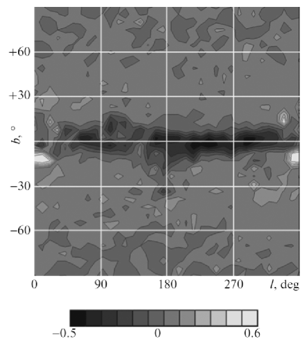
Figure 1: Differences between the reddening $E_{(B-V)G}$ from the G2010 map for stars with $1000<r<1600$ pc and $E_{(B-V)SFD98}$ from the SFD98 map as a function of $l$ and $b$. The black tone corresponds to a difference of $-0.5^{m}$. The isoline step is 0.1^m.

The same difference between the local and Galactic reddenings at low latitudes is seen as dark regions in Fig. 1, where the differences $E_{(B-V)G}-E_{(B-V)SFD98}$ are shown as a function of $l$ and $b$. The black tone corresponds to a difference of $-0.5^{m}$. The isoline step is 0.1^m. The vast regions of two predominant gray tones in the figure correspond to $-0.05^{m}<E_{(B-V)G}-E_{(B-V)SFD98}<0.15^{m}$. We see that the discrepancy between the maps at middle and high latitudes does not exceed 0.25^m. The mean difference is $0.06^{m}$. These differences are large enough to assume the existence of systematic differences between the maps.

Far from the equator, the dark tones in the figure corresponding to $E_{(B-V)G}<E_{(B-V)SFD98}$ are seen in the cloud complexes of the Gould Belt: the mid-latitude extension of the Aquila rift ($l\approx 15^{\circ}$, $b\approx+15^{\circ}$), Cepheus ($l\approx 110^{\circ}$, $b\approx+17^{\circ}$), Perseus and Orion ($l\approx 180^{\circ}$, $b\approx-30^{\circ}$), Chamaeleon ($l\approx 300^{\circ}$, $b\approx-16^{\circ}$), $\rho~{}Oph$ ($l\approx 354^{\circ}$, $b\approx+18^{\circ}$). In these regions, the SFD98 study revealed the maximum dust temperature gradient for middle latitudes and, as was shown by Arce and Goodman (1999), the resolution of the dust temperature map accompanying the SFD98 map is only $1.4^{\circ}$ rather than 6 arcmin, as for the main map. This should lead to a deviation of the SFD98 map from the true one in both directions at a steep temperature gradient. Indeed, several regions with $E_{(B-V)G}>E_{(B-V)SFD98}$ (light spots) are also noticeable near the mentioned regions and the Lupus complex ($l\approx 340^{\circ}$, $b\approx+13^{\circ}$).

The same effect apparently plays a role in the lightest regions in Fig. 1, $E_{(B-V)G}>E_{(B-V)SFD98}$. In fact, they form a ringlike region around the direction toward the Galactic center, but they do not affect the center itself (the light tones are especially pronounced at $l\approx 0^{\circ}$, $b\approx-10^{\circ}$ – this region is discussed below). The dust temperature gradient is also steep here. It apparently did not allow the SFD98 map to properly reflect the increase in reddening toward the Galactic center. At the same time, the G2010 map is saturated in these sky regions due to the limitation of the mapping method: the method is efficient only at $E_{(B-V)}<0.8^{m}$, because at high reddenings the F-type dwarfs and subgiants used in the method are mixed with red giants and red dwarfs on the $(J-Ks)$ – $Ks$ diagram. Closer to the Galactic center and at $|b|<5^{\circ}$, the SFD98 map is also saturated: although the possibility of such saturation was not pointed out by the authors directly, it is suggested both by the distribution of values with a jump near $E_{(B-V)}\approx 0.8^{m}$ and by the acknowledgment of the SFD98 authors that the influence of a large number of point IR sources is not ruled out near the Galactic equator. Thus, both maps deviate noticeably from the true one near the direction toward the Galactic center.

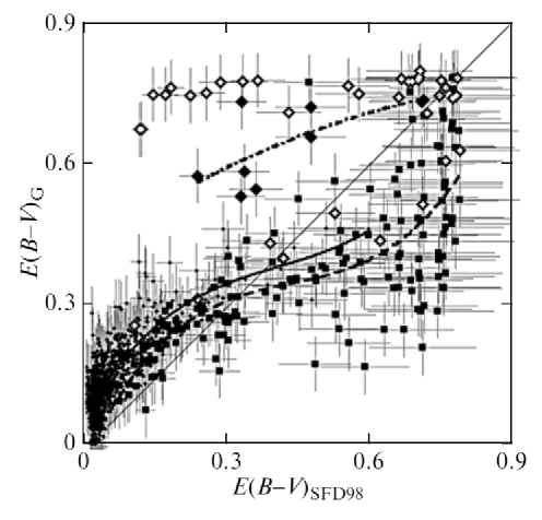
Figure 2: Correlation between $E_{(B-V)G}$ and $E_{(B-V)SFD98}$ for $10^{\circ}\times 10^{\circ}$ sky fields. The filled circles indicate the data for $|b|>15^{\circ}$ outside the clouds of the Gould Belt fitted by the solid curve. The large filled diamonds indicate the data for nine regions with $|b|>15^{\circ}$ containing the clouds of the Gould Belt fitted by the dash-dotted curve. The large open diamonds indicate the data for the region around the Galactic center ($-30^{\circ}<l<+30^{\circ}$, $|b|<15^{\circ}$). The squares indicate the data for $|b|<15^{\circ}$ far from the direction toward the Galactic center fitted by the dotted curve.

All of these features are also seen in Fig. 2, where the correlation between $E_{(B-V)G}$ and $E_{(B-V)SFD98}$ is shown for $10^{\circ}\times 10^{\circ}$ sky fields. The random errors are indicated for all data in the figure: 0.16% for SFD98 and 0.06^m for G2010 (obviously, the systematic errors somewhere exceed these estimates).

The data for $|b|>15^{\circ}$ outside the clouds of the Gould Belt are indicated by the filled circles (the main “swarm” of points is in the lower left corner of the figure). These were fitted by a polynomial using the least-squares method:

$$y=3x^{3}-3.7x^{2}+1.8x+0.06,$$ (10)

where $y$ is $E_{(B-V)G}$, $x$ is $E_{(B-V)SFD98}$. Thus, there exists a nonlinear relation between $E_{(B-V)G}$ and $E_{(B-V)SFD98}$: the SFD98 map underestimates the reddening at its low values, in particular, near the poles, by $0.06^{m}$ and overestimates it at $E_{(B-V)}>0.3^{m}$. The latter effect was detected by several authors (for references, see Cambresy et al. 2005). Arce and Goodman (1999) explain it by the fact that SFD98 used few galaxies with $E_{(B-V)}>0.15^{m}$ when calibrating $E_{(B-V)}$ from galaxies and, as a result, the SFD98 calibration at high reddenings is in error by a factor of 1.3–1.5. Cambresy et al. (2005) explain this effect by the properties of dust particles. All estimates from the literature are in good agreement with the data in Fig. 2, but a smooth systematic dependence is seen in this paper for the first time. The underestimation of the reddening near the poles by the SFD98 map is also explainable: the zero point of the SFD98 reddening scale is based on the assumption that there is no reddening near the poles.

The data for nine regions with $|b|>15^{\circ}$ containing the clouds of the Gould Belt are indicated in the figure by the large filled diamonds. These were fitted by the dependence indicated by the dash–dotted curve at the top of the figure. We see that here, as has been pointed out above, the SFD98 map underestimates significantly the reddening, while the G2010 map is close to saturation. It is important that the systematic dependence of $E_{(B-V)G}$ on $E_{(B-V)SFD98}$ here is parallel to dependence (10).

The large open diamonds in Fig. 2 indicate the data for the region around the Galactic center ($-30^{\circ}<l<+30^{\circ}$, $|b|<15^{\circ}$). Here, the G2010 map is saturated almost everywhere (the open diamonds at the top of the figure), while the SFD98 map is saturated only near the Galactic center (the open diamonds in the upper right corner of the figure).

The squares in Fig. 2 indicate the data for $|b|<15^{\circ}$ far from the direction toward the Galactic center. The saturation of the SFD98 map mentioned above is noticeable (the squares at the right edge of the figure). The dotted curve was drawn by the leastsquares method. The vertical shift of this curve from curve (10) is explained by the difference between the local (G2010) and total Galactic (SFD98) reddenings. The parallelism of all three curves in the figure suggests that the systematic error of the SFD98 map is the same over the entire sky.

Thus, the G2010 map is apparently more accurate than the SFD98 map in systematic terms and has a more accurate zero point (better estimates the reddening toward the poles), but the SFD98 map is more accurate near the Galactic center.

We will return to the data in Fig. 2 below when comparing our results with the 3D extinction map by Jones et al. (2011).

EXTINCTION AS THE PRODUCT OF REDDENING AND $R_{V}$

According to Eq. (1), the product of the G2010 stellar reddening map and the map of $R_{V}$ variations with allowance made for the relation $E_{(B-V)}=1.92E_{(J-Ks)}$ (Rieke and Lebofsky 1985) gives a map of interstellar extinction $A_{V}$.

The G2010 reddening map gives reliable data within about 1600 pc of the Sun at $|Z|<600$ pc (farther from the Galactic equator, the reddening depends almost entirely on the zero point determined with a large relative error – the reddening toward the Galactic poles). The G2012 map of $R_{V}$ variations gives reliable data only within no more than 600 pc of the Sun. However, the G2012 data suggest that the influence of local Galactic structures, the Gould Belt and the Local Bubble, with which the large $R_{V}$ variations near the Sun are apparently associated ceases at a greater distance. Consequently, at a greater distance, we can assume $R_{V}\approx 3.1$ far from the Galactic equator and a monotonic increase in this quantity along the $X$ coordinate toward the Galactic center in a thin layer (less than 150 pc in thickness) near the Galactic equator (G2012):

$$R\mathrm{v}=2.96+0.00025X.$$ (11)

At the expense of some reduction in accuracy and reliability, we thus extend the G2012 map of $R_{V}$ variations to the $2\times 2$ kpc region centered on the Sun: we adopt it as is within 600 pc of the Sun, dependence (11) in the layer $|Z|<100$ pc, and $R_{V}=3.1$ at the remaining locations. Accordingly, we use the G2010 reddening map and construct the extinction map in the $2\times 2$ kpc region centered on the Sun (remembering that the accuracy of the results decreases with increasing heliocentric distance).

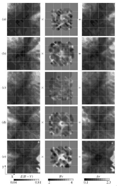
Figure 3: Contour maps of reddening $E_{(B-V)}$ (left column), coefficient $R_{V}$ (central column), and extinction $A_{V}$ (right column) as a function of the $X$ and $Y$ coordinates in the following layers: (a) $+150<Z<+250$ pc, (b) $+50<Z<+150$ pc, (c) $-50<Z<+50$ pc, (d) $-150<Z<-50$ pc, (e) $-250<Z<-150$ pc. The black tone corresponds to $E_{(B-V)}=0.04^{m}$, $R_{V}\leq 2$, $A_{V}=0.1^{m}$. The isoline step is $\Delta E_{(B-V)}=0.07^{m}$, $\Delta A_{V}=0.2^{m}$. $R_{V}\geq 4$ is marked by the white tone. The white lines of the coordinate grid are plotted with a 500-pc step. The Sun is at the centers of the plots. The Galactic center is on the right.

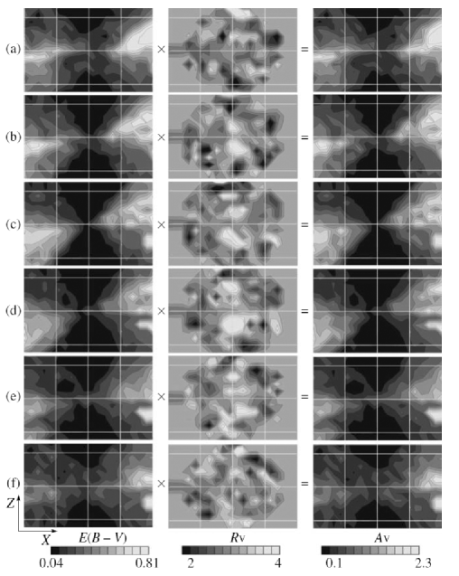
Figure 4: Same as Fig. 3, but the maps as a function of the $X$ and $Z$ coordinates in the following layers: (a) $+200<Y<+300$ pc, (b) $+100<Y<+200$ pc, (c) $0<Y<+100$ pc, (d) $-100<Y<0$ pc, (e) $-200<Y<-100$ pc, (f) $-300<Y<-200$ pc.

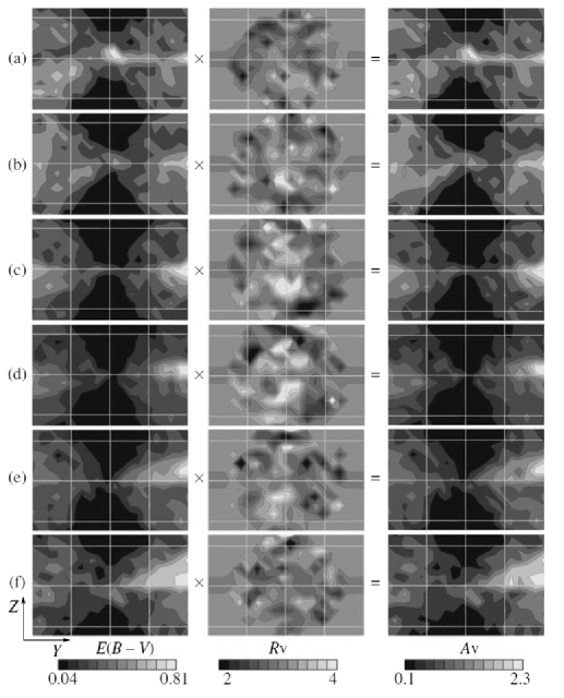
Figure 5: Same as Fig. 3, but the maps as a function of the $Y$ and $Z$ coordinates in the following layers: (a) $+200<X<+300$ pc, (b) $+100<X<+200$ pc, (c) $0<X<+100$ pc, (d) $-100<X<0$ pc, (e) $-200<X<-100$ pc, (f) $-300<X<-200$ pc..

Figure 3 shows the contour maps of reddening $E_{(B-V)}$ (left column), coefficient $R_{V}$ (central column), and extinction $A_{V}$ (right column) as a function of the $X$ and $Y$ coordinates in the following layers: (a) $+150<Z<+250$ pc, (b) $+50<Z<+150$ pc, (c) $-50<Z<+50$ pc, (d) $-150<Z<-50$ pc, (e) $-250<Z<-150$ pc. The black tone corresponds to $E_{(B-V)}=0.04^{m}$, $R_{V}\leq 2$, $A_{V}=0.1^{m}$. The isoline step is $\Delta E_{(B-V)}=0.07^{m}$, $\Delta A_{V}=0.2^{m}$. $R_{V}\geq 4$ is marked by the white tone. The white lines of the coordinate grid are plotted with a 500-pc step. The Sun is at the centers of the plots. The Galactic center is on the right. Similar maps are shown in Figs. 4 and 5, respectively, as a function of the $X$ and $Z$ coordinates in the layers (a) $+200<Y<+300$ pc, (b) $+100<Y<+200$ pc, (c) $0<Y<+100$ pc, (d) $-100<Y<0$ pc, (e) $-200<Y<-100$ pc, (f) $-300<Y<-200$ pc, and as a function of the $Y$ and $Z$ coordinates in the layers (a) $+200<X<+300$ pc, (b) $+100<X<+200$ pc, (c) $0<X<+100$ pc, (d) $-100<X<0$ pc, (e) $-200<X<-100$ pc, (f) $-300<X<-200$ pc.

The main thing that is seen on the presented extinction map is that at low and middle latitudes ($|b|<45^{\circ}$) it is determined mainly by the reddening map and not by the $R_{V}$ variations, no matter what extreme values this coefficient takes on; in contrast, the extinction at high latitudes is determined mainly by $R_{V}$. It is here that $R_{V}$ reaches its maximum values, exhibits large variations, and is determined with a lower accuracy. The role and uncertainty of $R_{V}$ at high latitudes are so great that today we even cannot assert with confidence that $R_{V}$ does not reach still higher values still farther from the Galactic plane, in unstudied regions, due to an increase in the fraction of coarse dust.

In any case, it is now clear that the low extinction and reddening at high latitudes in no way contradicts the high values of $R_{V}$ there. In addition, the numerous contradictory data on the correlation or anticorrelation between reddening and $R_{V}$ available in the literature now find an explanation. There is a correlation in a thin layer ($|Z|<100$ pc) near the Galactic equator, because both the reddening and $R_{V}$ increase here toward the Galactic center. Outside this layer, there is an anticorrelation: at high and middle latitudes, higher $R_{V}$ correspond to lower reddening. Obviously, all of this is determined by systematic differences in sizes and other properties of the dust grains in various regions of the Galaxy.

It is also important to estimate the contribution of the uncertainties in the reddening and $R_{V}$ to the total uncertainty in the extinction. Table 3 gives typical values of $E_{(B-V)}$, $R_{V}$, and $A_{V}$ as well as absolute and relative errors in these quantities toward the Galactic pole ($|b|\approx 90^{\circ}$), at a middle Galactic latitude ($|b|\approx 15^{\circ}$), and near the Galactic equator ($|b|\approx 0^{\circ}$) at a heliocentric distance of several hundred pc obtained in G2010, G2012, and this paper. The relative error in $A_{V}$ is equal to the quadratic sum of the relative errors in $E_{(B-V)}$ and $R_{V}$. Therefore, we see from the table that the error in $A_{V}$ is everywhere determined by the error in $E_{(B-V)}$, while, according to the most pessimistic estimates, the relative uncertainty in the variations of the extinction law, no matter what its nature is, does not exceed 10%. Therefore, this uncertainty does not affect the conclusions reached in G2010, G2012, and this paper and does not influence the accuracy of the constructed 3D extinction map at all latitudes.

In future, however, a refinement of the extinction law much more laborious than the construction of a 3D reddening map will come to the fore, because it will require reproducing the entire wavelength dependence of extinction. The latter is possible only by using homogeneous multiband photometry (spectrophotometry is better) for millions of stars with an accuracy of at least 0.01^m in the ultraviolet, visible, and IR ranges in many spatial cells of the Galaxy.

Table 3: Typical values of $E_{(B-V)}$, $R_{V}$, and $A_{V}$ as well as absolute and relative errors in these quantities at various latitudes at a heliocentric distance of several hundred pc obtained in G2010, G2012, and this paper

Parameter $$|b|\approx 90^{\circ}$$

0.06 0.20 0.70

0.06 0.06 0.06

1.00 0.30 0.09

4.20 3.10 2.80

0.20 0.20 0.20

0.05 0.06 0.07

Av 0.25 0.62 1.96

0.25 0.19 0.22

1.00 0.31 0.11

Since the main features of the G2010 reddening map discussed in the corresponding paper are also retained in the constructed extinction map, let us list them only briefly.

First of all, the Great Tunnel, a region of low reddening and extinction stretching in the figure from the top to the lower left corner, is seen in Fig. 3. The Great Tunnel was probably first mentioned by Welsh (1991) as an extension of the Local Bubble, a region of low gas density within about 100 pc of the Sun, toward Canis Major ($l\approx 230^{\circ}$). Gontcharov (2004) and Gontcharov and Vityazev (2005) showed that the concentration of high-luminosity stars, which, in fact, form the Gould Belt along the Tunnel edges, is enhanced along the Great Tunnel. Here, the large Scorpius, Perseus, Orion, and other cloud complexes are located along the Tunnel edges. All of this emphasizes the role of the Gould Belt as a dust container. In Fig. 4, the Gould Belt oriented in this plane at an angle of about 17^∘ to the Galactic plane is seen in the orientation of the largest absorbing structures (the light spots in the figure).

The region of high reddening and extinction seen as the white spot in Figs. 1, 3, and 4 ($l\approx 0^{\circ}$, $b\approx-10^{\circ}$, $X\approx 800$ pc, $Y\approx 0$ pc, $Z\approx-250$ pc, Sagittarius) has not been identified with any known structures. This may be an artifact that has emerged from the limitations of the method in a region with a steep reddening gradient.

The construction of a 3D extinction map in this paper offers great prospects for investigating individual cloud complexes, especially the distances to them and the relationship between reddening and $R_{V}$ in each complex. However, this extensive analysis is beyond the scope of this publication.

It is also impossible to compare the newly constructed map with the available numerous results referring to the extinction in specific regions of space in one publication. This work will be continued. Let us consider only one of the most interesting 3D extinction maps. It refers to the same region of space as the map obtained here but was constructed by a completely different method.

COMPARISON WITH THE 3D EXTINCTION MAP BY JONES et al.

Jones et al. (2011; below referred to as JWF11) constructed a 3D extinction map for high latitudes within 2 kpc of the Sun using the spectra of more than 9000 M-type dwarfs from the Sloan Digital Sky Survey (SDSS DR7) (Abazajian et al. 2009). The extinction was determined for each star by fitting its spectrum in the range $570<\lambda<920$ nm by a $\lambda$-dependent extinction curve. Unfortunately, the data show only the northern polar cap (approximately $b>50^{\circ}$), several narrow bands in the southern hemisphere, and isolated small zones of the sky. The data for 9362 stars from the JWF11 map were compared with the map constructed here in spherical segments with sizes $10^{\circ}\times 10^{\circ}\times 100$ pc in $l$, $b$, and $r$, respectively, containing at least ten JWF11 stars in each segment. This number is required to smooth out the $A_{V}$ variations from star to star (although the declared JWF11 accuracy of determining the individual $A_{V}$ was, on average, 0.04^m). Only the segments of the northern polar cap contain a sufficient number of stars from JWF11.

Our map is in good agreement with that from JWF11: for the spherical layers $+50<r<+150$, $+150<r<+250$ $+250<r<+350$ pc, the mean $A_{V}$ differences between our study and the JWF11 map are $-0.02^{m}$, $-0.01^{m}$ $0.02^{m}$, while the standard deviations of the differences are $0.11^{m}$, $0.07^{m}$ $0.10^{m}$, respectively. These agree with the accuracy estimates in this paper and JWF11. In other regions of space, the data are insufficient for comparison.

It is important that both maps at high latitudes give an equally high mean extinction ($\overline{A_{V}}\approx 0.2^{m}$) compared to the SFD98 map ($\overline{A_{V}}\approx 0.1^{m}$). This confirms the previously made assumption about the zeropoint error for the SFD98 map.

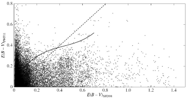
Figure 6: The correlation between $E_{(B-V)G}$ and $E_{(B-V)SFD98}$ for $10^{\circ}\times 10^{\circ}$, $|b|>15^{\circ}$ sky fields outside the clouds of the Could Belt from Fig. 2 is fitted by the solid curve (10). The correlation between $E_{(B-V)}$ for individual stars from the map by Jones et al. (2011) (with $E_{(B-V)}=A_{V}/3.1$) and $E_{(B-V)SFD98}$ is indicated by the open squares. The dashed curve indicates relation 1/1.

The dots in Fig. 6 represent the correlation of the JWF11 data for individual stars (with $E_{(B-V)}=A_{V}/3.1$) designated as $E_{(B-V)_{J}WF11}$ with the $E_{(B-V)SFD98}$ data, while the solid curve indicates dependence (10) presented above in Fig. 2 that fits the correlation between $E_{(B-V)G}$ and $E_{(B-V)SFD98}$ for $10^{\circ}\times 10^{\circ}$ and $|b|>15^{\circ}$ sky fields outside the clouds of the Gould Belt. The dashed curve indicates relation $E_{(B-V)_{J}WF11}=E_{(B-V)SFD98}$. We reached the following conclusions:

• The saturation of the SFD98 map mentioned above actually exists: the stars with $E_{(B-V)SFD98}>0.8^{m}$ are rare.

• The dots in the lower left corner of the figure, on the whole, agree with the solid curve, indicating a nonzero reddening at high latitudes ($\overline{E_{(B-V)}}=0.06^{m}$), as distinct from the SFD98 map.

• At $E_{(B-V)SFD98}>0.2^{m}$, almost all of the points lie below the solid curve, reflecting a deviation of the local reddening for comparatively close JWF11 stars from the total Galactic one derived from SFD98.

• At $E_{(B-V)SFD98}<0.2^{m}$, there are many stars with $E_{(B-V)_{J}WF11}\gg E_{(B-V)SFD98}$, which most likely suggests that the errors of these maps were disregarded at high latitudes.

• On the whole, the cloud of points is parallel to the solid curve, confirming that the systematic difference between the G2010 and SFD98 maps indicated by the curve is caused by the systematic error of the latter.

COMPARISON WITH 3D ANALYTICAL MODELS

Before the appearance of the G2009 extinction model, for many years the most widely used analytical 3D interstellar extinction model within the nearest kiloparsec had been the model by Arenou et al. (1992), which fits the mean extinction $A_{V}$ for 199 sky regions by parabolas as a function of the distance. The shortcoming of this model is the absence of any physical justification of the extinction variations.

When comparing our map with the model by Arenou et al., the mean difference turned out to be zero, while the standard deviation of the differences was 0.22^m for spatial cells closer than 500 pc and 0.19^m for cells closer than 400 pc.

Let us consider the correspondence between our map and the G2009 model. For this purpose, we will solve the system of equations (5), one equation for each spatial cell. The observed extinction $A_{V}$ is on the left-hand sides, while the function of $r$, $l$, and $b$ with the following 12 unknowns are on the righthand $\gamma$, $\lambda_{0}$, $Z_{A}$, $\zeta_{A}$, $Z_{0}$, $\zeta_{0}$, $A_{0}$, $A_{1}$, $A_{2}$, $\Lambda_{0}$, $\Lambda_{1}$, $\Lambda_{2}$. They are chosen so as to minimize the sum of the squares of the residuals of the left- and right-hand sides of Eqs. (5).

The calculations were performed for spatial cells within 500 pc of the Sun at $|Z|<300$ pc. Table 4 presents 12 unknowns and the standard deviation of the map from the model designated as $\sigma$. The “E” column provides data only for the equatorial layer with the characteristics giving the smallest deviation from the map; the “E+G” column provides data for both layers with the characteristics giving the smallest deviation from the map. For comparison, the “G2009” column presents the result obtained in G2009, while the $\sigma$ row gives two standard deviations – when fitting only by the equatorial layer and by both layers. The accuracies of determining the unknowns were estimated from the range of variations in the unknowns as the standard deviation increased significantly, by 0.004^m.

We see that the derived map is better described by the model with extinction in two layers rather than one, only equatorial layer.

Among the characteristics found, $A1$ $A2$ differ noticeably from those in G2009. In contrast, the difference between $A_{0}$ and $\Lambda_{0}$ was explained in G2009, where they are also significantly different in the solutions using different data: because of the low inclination of the Gould Belt to the Galactic equator and, accordingly, the small region of longitudes where the absorbing layers separate, only the total constant extinction is determined with confidence. This is also seen in the new solutions: the sum $A_{0}+\Lambda_{0}$ is almost the same in three columns of Table. 4 – 2.1^m, 2.2^m 2.35^m.

Thus, the constructed map agrees well with all of the models considered, but it agrees best with the G2009 model that allows for the extinction in the Gould Belt.

Table 4: Solutions of the system of equations (5)

Parameter G2009 E E+G

$$\gamma$$, deg

, deg

, pc

, pc

kpc

kpc

, deg

, pc

, pc

kpc

kpc

, deg

0.25/0.18 0.20 0.17

CONCLUSIONS

This is the fourth paper in our series of studies of the interstellar extinction in the Galaxy. As our previous studies (G2009, G2010, G2012), it shows that the stellar reddening and extinction can be analyzed using accurate multicolor broadband photometry from present-day surveys of millions of stars and that the Gould Belt plays a great role as a region containing absorbing matter in clouds oriented approximately radially with respect to the Sun.

The product of the stellar reddening map (G2010) by the map of $R_{V}$ variations (G2012) allows an extinction map within the nearest kiloparsec from the Sun to be constructed with a spatial resolution of 50 pc and an accuracy $\sigma(A_{V})=0.2^{m}$. At present, there are high-resolution and high-accuracy 2D extinction maps (e.g., SFD98), high-resolution and high-accuracy 3D maps for part of the sky (e.g., JWF11), and fairly accurate all-sky 3D maps farther than 2 kpc from the Sun. The map presented here is currently one of the few 3D maps for the entire nearest kiloparsec.

Both theoretical calculations and data analysis point to a great role of the absorbing matter within the nearest kiloparsec: it determines the extinction in the bulk of the sky and is particularly important for estimating the extinction toward extragalactic objects.

The limited volume of the paper forces us to compare the constructed reddening and extinction maps primarily with the most popular results: the SFD98 reddening map and the analytical extinction models by Arenou et al. (1992) and G2009. In all cases, good agreement was found, but we showed that the SFD98 map has saturation near the Galactic equator, systematic errors in regions with a high reddening, and a zero-point error, while the analytical extinction model benefits if the extinction in the Gould Belt is explicitly taken into account.

In the constructed extinction map, we found no systematic errors nowhere except the region around the direction toward the Galactic center.

Our extinction map showed that it is determined mainly by reddening variations at low and middle latitudes ($|b|<45^{\circ}$) and by $R_{V}$ variations at high latitudes. Since it is here that $R_{V}$ reaches its maximum values, exhibits large variations, and is determined with a lower accuracy, its refinement is needed. In this paper, we explain for the first time the contradictory data on the correlation or anticorrelation between reddening and $R_{V}$ available in the literature. There is a correlation in a thin layer ($|Z|<100$ pc) near the Galactic equator, because both the reddening and $R_{V}$ increase here toward the Galactic center. There is an anticorrelation outside this layer: higher values of $R_{V}$ correspond to lower reddening at high and middle latitudes. Obviously, all of this is determined by systematic differences in sizes and other properties of the dust grains in different regions of the Galaxy.

Since the largest structures within the nearest kiloparsec, including the Local Bubble, the Gould Belt, the Great Tunnel, the Scorpius, Perseus, Orion, and other complexes, have manifested themselves in the constructed map, its comprehensive analysis and refinement offer great prospects for investigating these structures, especially the distances to them and the local dust properties.

References

- 1. K.N. Abazajian, J. K. Adelman-McCarthy, M. A. Agueros, et al., Astrophys. J. Suppl. Ser. 182, 543 (2009).
- 2. H.G. Arce, A.A. Goodman, Astrophys. J. 512, L135 (1999).
- 3. F. Arenou, M. Grenon, A. Gomez, Astron. Astrophys. 258, 104 (1992).
- 4. L. Cambresy, T.H. Jarrett, C.A. Beichman, Astron. Astrophys. 435, 131 (2005).
- 5. G.A. Gontcharov, Astron. Soc. Pacif. Conf. Proc., 316, 221 (2004).
- 6. G. A. Gontcharov, Astron. Lett. 35, 780 (2009).
- 7. G. A. Gontcharov, Astron. Lett. 36, 584 (2010).
- 8. G. A. Gontcharov, Astron. Lett. 38, 12 (2012).
- 9. G. A. Gontcharov and V. V. Vityazev, Vestn. SPb. Univ., Ser. 1 3, 127 (2005).
- 10. E. Høg, C. Fabricius, V.V. Makarov, et al., Astron. Astrophys. 355, L27 (2000).
- 11. D.O. Jones, A.A. West, J.B. Foster, Astron. J. 142, 44 (2011).
- 12. P. P. Parenago, A Course of Stellar Astronomy (GITTL,Moscow, 1954) [in Russian].
- 13. M. Perryman, Astronomical application of astrometry (Cambridge Univ. Press, Cambridge, 2009).
- 14. G.H. Rieke, R.M. Lebofsky, Astrophys. J. 288, 618 (1985)
- 15. A.C. Robin, C. Reyle, S. Derriere, et al., Astron. Astrophys. 409, 523 (2003).
- 16. D.J. Schlegel, D.P. Finkbeiner, M. Davis, Astrophys. J. 500, 525 (1998).
- 17. M.F. Skrutskie, R.M. Cutri, R. Stiening, et al., Astron. J. 131, 1163, (2006), http://www.ipac.caltech.edu/2mass/releases/allsky/index.html.
- 18. B.Y. Welsh, Astrophys. J. 373, 556 (1991).