Magnetic field dependence of excitations near spin-orbital quantum criticality

Abstract

The spinel FeSc₂S₄ has been proposed to realize a near-critical spin-orbital singlet (SOS) state, where entangled spin and orbital moments fluctuate in a global singlet state on the verge of spin and orbital order. Here we report powder inelastic neutron scattering measurements that observe the full bandwidth of magnetic excitations and we find that spin-orbital triplon excitations of an SOS state can capture well key aspects of the spectrum in both zero and applied magnetic fields up to 8.5 T. The observed shift of low-energy spectral weight to higher energies upon increasing applied field is naturally explained by the entangled spin-orbital character of the magnetic states, a behavior that is in strong contrast to spin-only singlet ground state systems, where the spin gap decreases upon increasing applied field.

When magnetic ions posses an orbital degeneracy in addition to spin, the combined effects of the on-site spin-orbit coupling and the inter-site magnetic exchange interactions have been theoretically proposed to stabilize correlated states with entangled spin-orbital character and novel quasiparticles Chen et al. (2009a); Khaliullin (2013). Generally such physics is not directly experimentally accessible as symmetry-lowering Jahn-Teller (JT) structural distortions Jahn and Teller (1937) tend to lift orbital degeneracy leaving a spin-only degree of freedom. However, in the case of relatively strong spin-orbit coupling, or certain crystal structures where JT distortions are inhibited by the lattice geometry, spin-orbit entanglement can become manifest. For $d^{4}$ Khaliullin (2013) and $d^{6}$ Low and Weger (1960) transition metal ions in certain high-symmetry crystal environments the single-ion ground state is a spin-orbit entangled $J_{\rm eff}=0$ singlet with an excited $J_{\rm eff}=1$ triplet at higher energy. In this case, a theoretically-proposed phase diagram Chen et al. (2009a) as a function of the ratio $x$ of magnetic exchange couplings to the singlet-triplet gap $\lambda$ is shown in Fig. 1. Cooperative spin and orbital order is expected for $x>x_{c}$, with a novel amplitude (“Higgs”) mode for $x\gtrsim x_{c}$ Khaliullin (2013); Jain et al. and entangled spin-orbital fluctuations present at the critical point $x_{c}$. In the regime of moderate exchange interactions, $x\lesssim x_{c}$, spins and orbitals are expected to be strongly fluctuating in a quantum paramagnetic state denoted as a “spin-orbital singlet” (SOS), with strong correlations between sites Chen et al. (2009a). Even though the SOS state has no spin or orbital order, it supports quasiparticles, so called “spin-orbital triplons” (or “spin-orbitons” Mittelstädt et al. (2015)), corresponding to isotropically-polarized, spin and orbital density wave packets that can propagate coherently across the lattice.

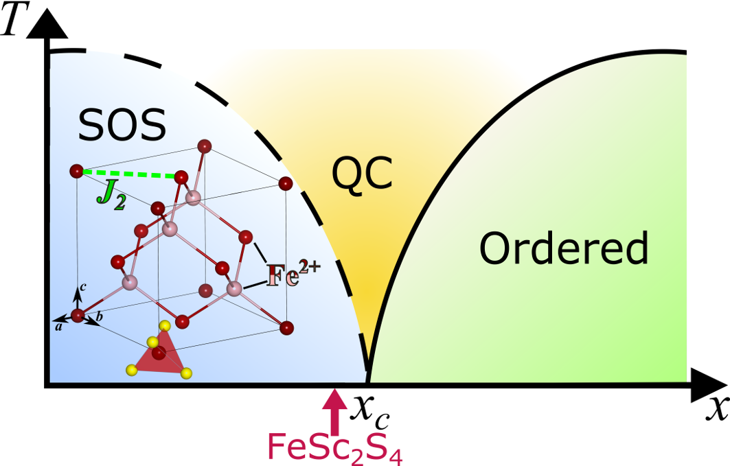
Figure 1: (Color online). Generic phase diagram as a function of $x=J_{2}/\lambda$ Chen et al. (2009a) with location of FeSc₂S₄ indicated by the vertical arrow. Labels SOS, QC and Ordered stand for spin-orbital singlet, quantum critical, and spin and orbitally ordered, respectively. Solid/dashed line indicates a phase transition boundary/crossover. Inset shows Fe²⁺ ions in FeSc₂S₄ are locally coordinated by a regular tetrahedron (red shaded polyhedron) of S^2- atoms (yellow balls) and are arranged in two FCC sublattices (light/dark red balls) with intra-sublattice NN AFM exchange $J_{2}$.

The spinel FeSc₂S₄ has been proposed Fritsch et al. (2004); Krimmel et al. (2005); Chen et al. (2009a) as a unique candidate to display a SOS state with intermediate-strength exchange interactions ($x\lesssim x_{c}$) that bring it almost on the verge of spin and orbital order. It is the only known system to explore the physics of highly-dispersive spin-orbital triplons, that may be close to spin-orbital quantum criticality. Here we report inelastic neutron scattering (INS) measurements over the full bandwidth of the magnetic excitations and we find good agreement with the expected spectrum of spin-orbital triplons of a near-critical SOS state. In applied magnetic field we observe a striking shift of the low-energy spectral weight to higher energies, a direct fingerprint of the entangled spin-orbital character of the magnetic states.

FeSc₂S₄ has a cubic crystal structure with space group $Fd\bar{3}m$ (no. 227) and lattice parameter $a=10.51$ Å at 300 K Tomas and Guittard (1979). Fe²⁺ ions are tetrahedrally-coordinated by S^2- and in this crystal field of cubic symmetry the one-electron $d$ orbital states of Fe²⁺ are split into a lower $e$-doublet and upper $t_{2}$-triplet. Hund’s coupling stabilizes a high-spin ($S=2$) state, $e^{3}t_{2}^{3}$, with a two-fold orbital degeneracy. The atomic spin-orbit interaction $\lambda_{0}\bm{L}\cdot\bm{S}$ lifts this two-fold orbital and five-fold spin degeneracy to stabilize a SOS ground state with wavefunction Low and Weger (1960)

$$\frac{1}{\sqrt{2}}|3z^{2}-r^{2}\rangle|0\rangle+\frac{1}{2}|x^{2}-y^{2}\rangle\left(|-2\rangle+|+2\rangle\right),$$ (1)

where for each term the first ket gives the (multi-electron) orbital state and the second ket the $S_{z}$ eigenvalue. The first excited state is a triplet above a gap $\lambda$ and local singlet-triplet transitions then form the key ingredient from which coherently-propagating triplons develop in the presence of inter-site exchange interactions.

Previous susceptibility, specific heat and NMR measurements on FeSc₂S₄ Büttgen et al. (2006); Fritsch et al. (2004) showed no clear anomalies indicative of spin or orbital order in spite of strong magnetic interactions manifested by a large antiferromagnetic (AFM) Curie-Weiss temperature of $-45$ K, indicating that the material may indeed be in the SOS phase. INS studies Krimmel et al. (2005) focusing on the very low energy dynamics indicated that the dominant magnetic interaction is an AFM exchange $J_{2}$ between spins located at next-nearest neighbor (NNN) sites. This splits the diamond lattice into two magnetically-decoupled, frustrated FCC lattices (light/dark sites in Fig. 1), where $J_{2}$ acts on NN bonds.

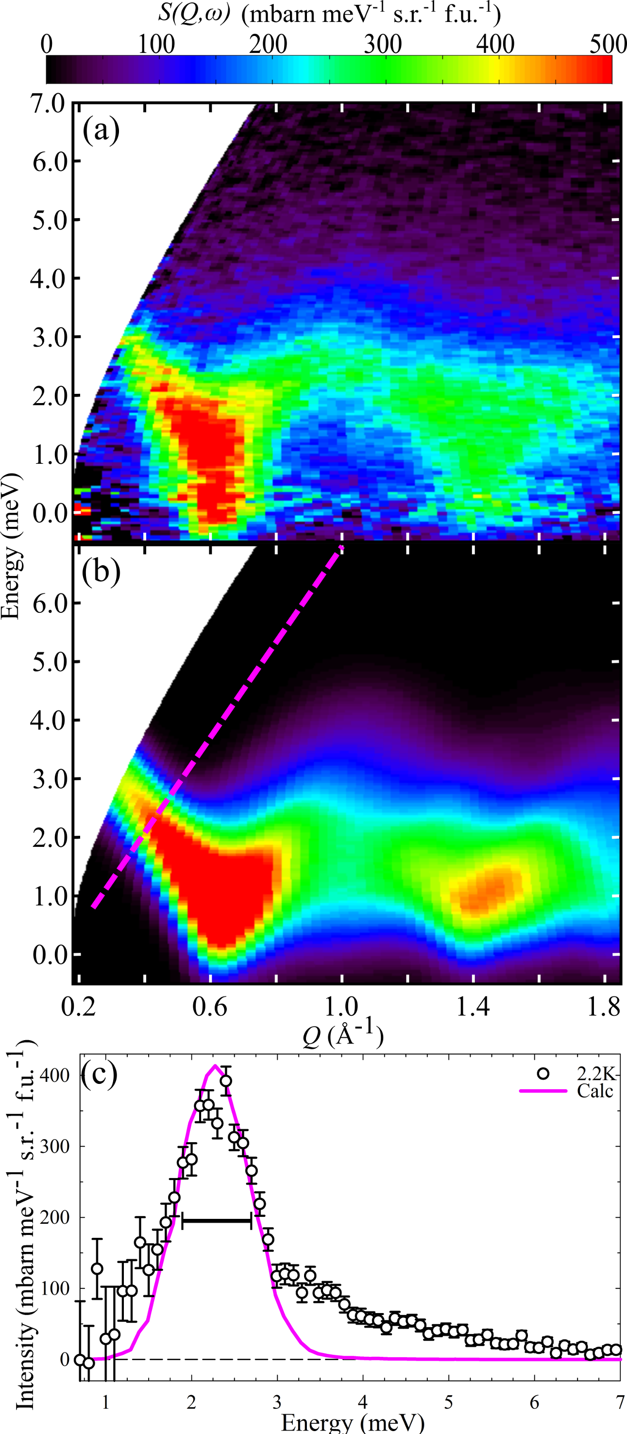
Figure 2: (Color online). (a) Background subtracted (see sup ) zero field INS data observing highly dispersive magnetic excitations (MERLIN, $E_{i}$=15 meV, 12 h counting time, energy resolution 0.79 meV FWHM on the elastic line). (b) Corresponding one-triplon spectrum including convolution with the instrumental resolution. (c) Intensity along the tilted dashed line direction in (b), compared to the model calculation (solid line). Horizontal bar indicates expected peak FWHM due to instrumental resolution and spherical averaging.

We have probed the magnetic excitations using INS measurements first in zero magnetic field and at temperatures 2.2-50 K using the direct-geometry, time-of-flight spectrometer MERLIN at the ISIS neutron source Bewley et al. (2006). The sample was a 4 g powder of FeSc₂S₄ synthesized as described in sup and used in previous thermodynamic and diffraction studies Fritsch et al. (2004). The INS intensities were converted into absolute units by normalization to data measured on a vanadium standard. For incident neutrons of energy $E_{i}=15$ meV the covered phase space observed the full bandwidth of magnetic excitations, which showed prominent dispersions with a bandwidth extending to around 4 meV at the lowest temperatures, as shown in Fig. 2(a). The high-temperature data was used to parameterize and subtract the non-magnetic background (as described in sup ), such that Fig. 2(a) shows the magnetic signal only. Within experimental uncertainty no additional magnetic transitions were detected at higher energy transfers (data collected using incident neutron energies up to 200 meV). This is consistent with the expectation that the single-ion ground state is close to the SOS wavefunction in (1), for which no other (crystal-field) transitions are symmetry allowed sup . In agreement with previous low-energy studies Krimmel et al. (2005), we observe a softening of the magnetic excitations near a critical wavevector $Q_{S}\approx 0.6$ Å^-1 [see Fig. 2(a)], whose magnitude coincides with the structurally-forbidden $(100)$ reciprocal lattice position (in units of $2\pi/a$) and a natural wavevector for AFM ordering on the FCC lattice Chen et al. (2009a). Higher-resolution measurements shown in Fig. 3(a) indicate a clear suppression of scattering weight below $\sim$0.4 meV, indicating that the gap is much smaller than the full bandwidth of the magnetic excitations extending to around 4 meV. This is consistent with the proposal that FeSc₂S₄ is in the very close proximity of the critical point between SOS and magnetic/orbital order, at which the gap would be expected to close Chen et al. (2009a).

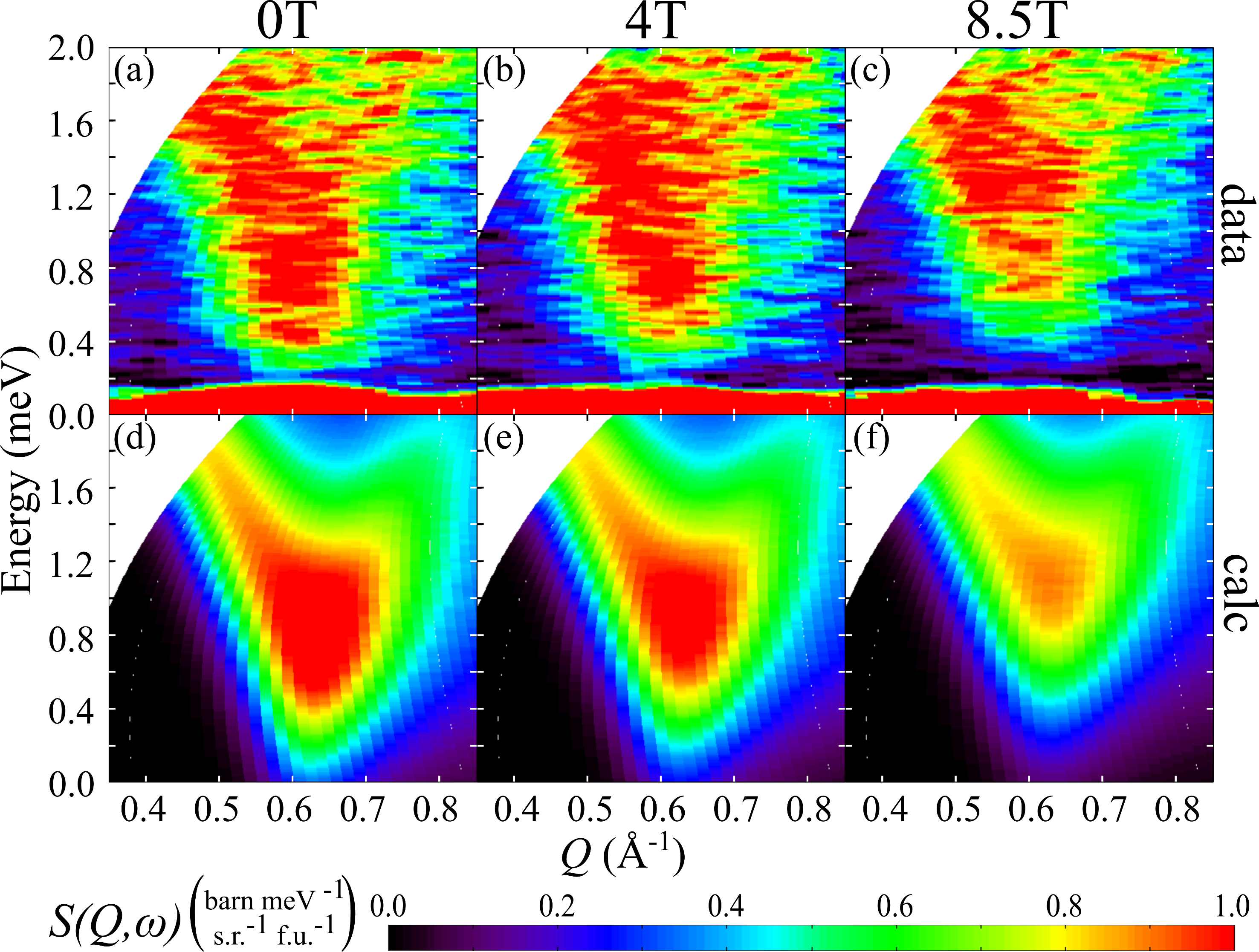
Figure 3: (Color online) (a-c) Background-subtracted INS data at 0, 4 and 8.5 T magnetic field compared with model calculations (d-f), respectively. The data was collected using FOCUS with $E_{i}=3.27$ meV, elastic line energy resolution 0.18 meV FWHM and 11 h counting per setting.

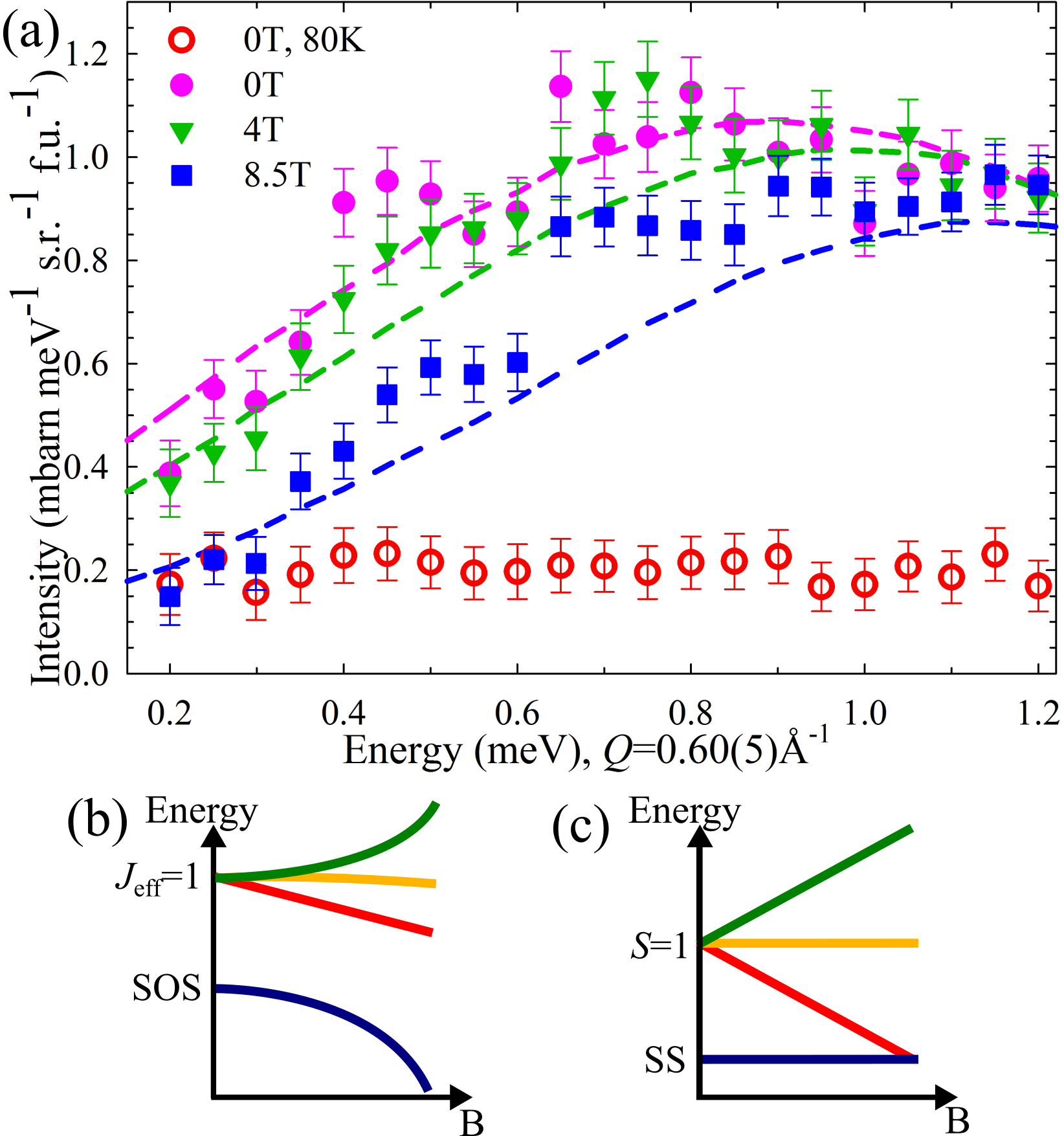
Figure 4: (Color online) (a) Energy scan at the softening wavevector $Q_{S}$ through the background subtracted data in Fig. 3(a-c): filled circles, triangles and squares denote fields of 0, 4 and 8.5 T, respectively. Dashed lines are the model calculations shown in Fig. 3(d-f). Data at 0 T in the paramagnetic phase at high temperatures (80 K) is also included (red open circles). b) Schematic of the ground and excited states’ energies as a function of applied field in the case of a SOS and (c) a spin-singlet system.

The magnetic field dependence of the excitations was measured on the same powder sample using the FOCUS time-of-flight spectrometer at the Swiss Spallation Neutron Source SINQ (PSI) with the sample placed inside a vertical 9 T cryomagnet. The obtained magnetic INS signal is plotted in Figs. 3(a-c). By comparing the data at different fields it is apparent that the intense V-shaped magnetic signal near $Q_{S}$ shifts upwards upon increasing field. This trend is directly seen in the energy scan in Fig. 4(a) by comparing the data at 0, 4 and 8.5 T, spectral weight moves to higher energies upon increasing field.

Below we compare quantitatively the dispersive features of the excitation spectrum and the observed magnetic field dependence of the low-energy scattering with a model of spin-orbital triplons of a SOS ground state. In zero field the triplon dispersion derived in the harmonic approximation using pseudo-boson operators sup or alternative methods Ish and Balents (2015) is

$$\hbar\omega(\bm{k})=\lambda\sqrt{1+\frac{4J(\bm{k})}{\lambda}},$$ (2)

where $J(\bm{k})=J_{2}\sum_{\bm{A}}\cos(\bm{k}\cdot\bm{A})$ is the Fourier transform of the exchange couplings and $\bm{A}$ runs over all NN vectors of an FCC sublattice. The local singlet-triplet gap $\lambda$ is determined by the crystal field strength parameterized (using standard convention Abragam and Bleaney (1970)) by the single parameter $B_{4}<0$, and the atomic spin-orbit coupling $\lambda_{0}<0$. Within a minimal ($J_{2}$,$B_{4}$,$\lambda_{0}$) model we calculate the powder-averaged INS spectrum including the triplons’ dynamical structure factor (for details see sup ) and compare systematically with scans through the INS data as shown in Figs. 2(c) and 4(a) (magenta filled symbols). In addition, we require the model parameters to reproduce optical data: the sharp 4.46 meV absorption in THz spectroscopy Laurita et al. (2015); Mittelstädt et al. (2015), identified with the triplon energy (2) at the zone center, $\hbar\omega(\bm{0})=\sqrt{\lambda(\lambda+48J_{2})}$, and the sharp optical absorption at $\hbar\Omega=262(2)$ meV, attributed to the transition from the ground state to the lowest level of the upper orbital triplet not (a). Using those multiple constraints the best fit parametrization is obtained for $J_{2}=0.136(6)$ meV, $B_{4}=-2.45(6)$ meV and $\lambda_{0}=-12.1(1)$ meV, which give $\lambda=2.28(6)$ meV not (b). This parametrization reproduces (by construction) the energies of both optical transitions and the $J_{2}$ value is comparable to that deduced from Curie-Weiss fits of the high-temperature susceptibility Laurita et al. (2015) and estimated from density-functional calculations Sarkar et al. (2010). The $B_{4}$ and $\lambda_{0}$ values are comparable with $-2.58$ and $-10.0(9)$ meV, respectively, found for Fe²⁺ ions in FeCr₂S₄ Feiner (1982).

The INS spectrum for the fitted parameter values is shown in Fig. 2(b), where we have also included an intrinsic linewidth broadening $\sim$1 meV, a possible significance of this broadening will be discussed later. The parametrization by the minimal model captures well the key features of the INS data with clear V-shaped dispersions and mode softenings near 0.6 and 1.4 Å^-1, identified with scattering emanating near the reciprocal lattice positions (100) and (211), respectively. A corresponding calculation performed for the data measured on FOCUS at zero field is shown in Fig. 3(d) and this also compares well with the data in panel (a). Energy scans near the softening wavevector are in good agreement between the data and model [see Fig. 4(a), magenta filled symbols/line]. Fig. 2(c) shows also the limitations of the present model. The energy scan shown cuts across the low-$Q$ dispersion and the model (solid line) reproduces well the observed peak position. However, the linewidth is broader than expected based on resolution effects alone (horizontal bar) and there is considerable additional continuum scattering intensity at higher energies above 3 meV, which we attribute to multi-triplon scattering events, not included in the present model.

With the model parameters kept fixed by the fits to zero-field data, we now calculate the expected behavior in an external magnetic field, which contributes additional terms to the single-ion Hamiltonian; $\mu_{B}\bm{B}\cdot(\bm{L}+2\bm{S})+12J_{2}\bm{S}\cdot\langle\bm{S}\rangle$. The first term is the Zeeman energy in field and the second term includes the effect of the exchange interactions, treated in a mean-field approximation Chen et al. (2009b). $\langle\bm{S}\rangle$ is the field-induced spin polarization of the ground state, i.e. $\langle\bm{S}\rangle=\langle\psi_{0}|\bm{S}|\psi_{0}\rangle$, where $\psi_{0}$ is the ground state wavefunction of the single-site Hamiltonian. Solving for $\langle\bm{S}\rangle$ self-consistently we find the wavefunctions $\psi_{1,2,3}$ and energies $\lambda_{1,2,3}$ for a general field direction, determine the triplon dispersion relations and neutron structure factor, then average the spectrum over a spherically uniform distribution of powder grains (see sup for details). The model calculations are compared with the measured INS data in Fig. 3, panels (e-f) with (b-c) at 4 and 8.5 T; the model captures the apparent upwards shift of the scattering intensity upon increasing field. This is even more clearly seen in the energy scans in Fig. 4(a), the model calculation (dashed lines) reproduce well the observed shift of spectral weight to higher energies upon increasing field with no adjustable parameters once the overall intensity scale factor is fixed by the comparison in zero field.

It is insightful to compare the spin-orbital triplons of a SOS ground state discussed here with triplons of a spin-singlet (SS) ground state with completely quenched orbital degree of freedom, as found for example in quantum dimerized antiferromagnets like TlCuCl₃ Rüegg et al. (2008). For the latter, a magnetic field Zeeman splits the triplet into $S_{z}=-1,0,+1$ states, with a linear reduction in the gap to the $S_{z}=-1$ state, as shown schematically in Fig. 4(c). At a critical field level crossing with the ground state occurs and magnetic order ensues via condensation of triplons. One might wonder how the behavior of spin-orbital triplons can be any different; the triplons now have an effective angular momentum $J_{\rm eff}=1$ (as opposed to $S=1$ in the SS case). A low applied magnetic field Zeeman splits the triplet into $J_{\rm{eff},z}=-1,0,+1$ states Low and Weger (1960); Laurita et al. (2015), however at higher fields terms quadratic and higher in $B$ prevail Ish and Balents (2015); not (c) and allow mixing between the SOS and the $J_{\rm{eff},z}=0$ triplet mode. This enables the ground state to reduce its energy in applied field by acquiring a finite polarization along the field direction, see Fig. 4(b), thus avoiding magnetic order via level crossing with the triplet states.

We now relate our results to the generic phase diagram in Fig. 1, describing the transition from SOS to magnetic/orbital order upon increasing $x=J_{2}/\lambda$. Using the parameters obtained from fitting the INS data yields $x\simeq 0.060$, marginally close to the proposed critical value $x_{c}=1/16$. For such close proximity to criticality one might expect manifestations of enhanced quantum fluctuations associated with the critical point. For $x\lesssim x_{c}$ in addition to sharp triplon excitations one would also expect multi-triplon continua at higher energies, with enhanced spectral weight and decreasing gap as $x\nearrow x_{c}$, with the triplon dispersions becoming lower boundaries of a critical continuum of excitations precisely at the quantum critical point at $x_{c}$. Effects associated with such continuum scattering and/or broadening of sharp modes may be at least partly responsible for the extra scattering intensity and broadening effects observed in the INS data in Fig. 2(c), we hope our results will stimulate further theoretical modelling of such effects close to spin-orbital quantum criticality.

One may ask if other materials may exhibit related physics. We note that a high-spin $d^{4}$ ion (e.g. Mn³⁺) in an octahedral (weak) cubic crystal field displays the same single-ion physics (electron analogue) as Fe²⁺ in FeSc₂S₄, i.e. spin $S=2$ and two-fold orbital degeneracy, where the spin-orbit coupling (now $\lambda_{0}>0$) stabilizes the SOS ground state in (1) with a $J_{\rm eff}=1$ excited triplet. Similar singlet-triplet physics, but with a singlet ground state distinct from (1), originating from $S=1$ and three-fold orbital degeneracy, is expected for low-spin $d^{4}$ ions (e.g. Ru⁴⁺) in strong octahedral crystal field Khaliullin (2013); Jain et al. and $d^{8}$ ions (e.g. Ni²⁺) in tetrahedral field not (d). If such ions can resist JT distortions, they are candidates to display correlated spin-orbit states under inter-site exchange, potentially in a different part of the phase diagram in Fig. 1.

To summarize, we have reported powder INS measurements of the full bandwidth of magnetic excitations in the spinel FeSc₂S₄ and have found that that the key dispersive features can be well described by spin-orbital triplons of a near-critical SOS state. In high applied magnetic field we have observed a shift of spectral weight to higher energies, giving support to the theoretical proposal Chen et al. (2009b) that applied fields further stabilize the SOS state by moving the system away from the quantum critical point, this is a direct consequence of the entangled spin-orbital nature of the ground and excited triplet states.

Note added. As this work was being completed Ref. Plumb et al. (2016) appeared, reporting evidence for marginal magnetic order in samples synthesized using a different protocol, suggesting an extreme sensitivity to the synthesis route. Broadly speaking, there are three main physical factors that could lead to such a discrepancy; vacancies, site disorder, and off-stoichiometry, all of which are discussed in the Supplemental Material sup . We conclude that off-stoichiometry can lead to magnetic order with a transition temperature of a few K. Our results highlighting that magnetic fields favor the SOS state suggest a very interesting possibility that fields applied onto an ordered sample, potentially along a particular direction in a single crystal, may drive it towards the SOS state and thus reach the long-searched-for quantum critical point.

I Supplemental Material

Here we outline 1) the derivation of the spin-orbital wavefunctions for a single Fe²⁺ ion in a tetrahedral cubic crystal field including spin-orbit coupling, 2) the description of the lowest singlet-triplet transition in terms of spin-orbital triplon operators, 3) the analytic derivation of the triplon dispersions in the presence of magnetic exchange interactions and the relevant matrix elements for neutron scattering, 4) the derivation of single-ion states in the presence of an external magnetic field and exchange via a mean-field approach, 5) the non-magnetic background subtraction procedure for the INS data via the principle of detailed balance, 6) the derivation of the neutron cross-section for triplon scattering and spherical averaging to compare with powder INS data, and 7) details on the sample preparation for the FeSc₂S₄ powder used in the INS experiments.

II S1. Single Ion Hamiltonian

This section outlines the derivation of the spin-orbital wavefunctions for a singe Fe²⁺ ($3d^{6}$) ion in the (weak) crystal field environment appropriate for FeSc₂S₄. The Hamiltonian is

$$\mathcal{H}=\mathcal{H}_{\rm cf}+\mathcal{H}_{\rm SO}+\mathcal{H}_{\text{Zeeman}},$$ (S1)

where the three terms are the crystal field, spin-orbit and external magnetic field contributions, respectively. The crystal-field term can be expressed via the equivalent operator method in terms of Stevens operators of the orbital angular momentum $\bm{L}$. The allowed terms are constrained by the local site symmetry and for a cubic environment $\mathcal{H}_{\rm cf}$ is of the form Abragam and Bleaney (1970)

$$\mathcal{H}_{\rm cf}=B_{4}(O_{4}^{0}+5O_{4}^{4}),$$

where $O_{4}^{0}$ and $O_{4}^{4}$ are Stevens operators (tabulated in Hutchings (1964)) and $B_{4}$ is a constant that characterizes the strength of the crystal field ($B_{4}<0$ for a $d^{6}$ ion in tetrahedral coordination). In expanded form the crystal-field Hamiltonian reads

$$\begin{array}[]{ll}\mathcal{H}_{\rm cf}=B_{4}([35L_{z}^{4}-30L(L+1)L_{z}^{2}+25L_{z}^{2}\\ ~{}~{}-6L(L+1)+3L^{2}(L+1)^{2}]+\frac{5}{2}[L_{+}^{4}+L_{-}^{4}]),&\end{array}$$ (S2)

where the Cartesian $x,y,z$ axes are chosen along the cubic axes of the unit cell.

The second term in (S1) is the atomic spin-orbit interaction,

$$\mathcal{H}_{\rm SO}=\lambda_{0}\bm{L}\cdot\bm{S},$$ (S3)

with $\lambda_{0}<0$ for a $d^{6}$ ion (hole-like). For calculation purposes it is helpful to expand the dot product as

$$\bm{L}\cdot\bm{S}=L_{z}S_{z}+\frac{1}{2}\left(L_{+}S_{-}+L_{-}S_{+}\right),$$

where the $\pm$ ladder operators are the standard ones, i.e. $L_{\pm}|L,M_{L}\rangle=\sqrt{(L\mp M_{L})(L\pm M_{L}+1)}|L,M_{L}\pm 1\rangle$ and similar for $S_{\pm}$.

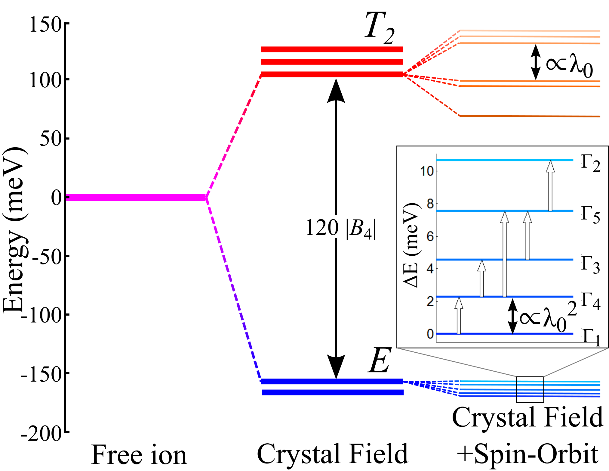
Figure S1: (Color online) Splitting of Fe²⁺ free ion orbital levels due to crystal field and spin-orbit coupling. Inset: Allowed transitions via neutron scattering for the 5 states derived from the $E$-doublet where side labels $\Gamma_{1-5}$ indicate the corresponding irreducible representations (from Testelin et al. (1992)).

The Fe²⁺ ($3d^{6}$) ions are in an $S=2$, $L=2$ configuration. We use the $|M_{L},M_{S}\rangle$ states as basis to describe the wavefunctions, where $M_{L}$ and $M_{S}$ are the projections of the $\bm{L}$ and $\bm{S}$ operators onto the quantization axis $z$, each takes values of $-2\dots 2$. In this basis all operators are represented by $25\times 25$ matrices and diagonalization of the Hamiltonian (S1) obtains the spectrum of states shown in Fig. S1. The cubic crystal field splits the 5-fold degenerate $L=2$ orbital states into a lower $E$-doublet and upper $T_{2}$-triplet above a gap $\Delta_{\rm cf}=-120B_{4}>0$ (same level splitting, symmetry of wavefunctions and order of levels as for a single $d$-electron with orbital quantum number $l=2$). The spin-orbit coupling further splits those levels. At lowest order in $\lambda_{0}$, the upper $T_{2}$ manifold is split into three levels with energies $\Delta_{\rm cf}-3\lambda_{0}$, $\Delta_{\rm cf}-\lambda_{0}$ and $\Delta_{\rm cf}+2\lambda_{0}$, and the $E$ manifold is split into 5 equidistant levels separated by $6\lambda_{0}^{2}/\Delta_{\rm cf}$ Low and Weger (1960). The last column in Fig. S1 indicates those lowest five levels and their irreducible representations, the ground state is a singlet and the first excited state a triplet. Transitions between states probed via neutron scattering are determined by the matrix element

$$\langle f|\bm{L}+2\bm{S}|i\rangle,$$ (S4)

where $|i\rangle$ and $|f\rangle$ denote the initial and final states, respectively. The symmetry-allowed transitions between levels originating from the lower $E$-doublet are indicated by thick white arrows in Fig. S1 last column.

Note that the three degenerate states of the first excited triplet can be described by an effective angular momentum $J_{\text{eff}}=1$ with $\psi_{1,2,3}$ identified as eigenstates of $J_{\text{eff},z}$ with eigenvalues of $-1,0,+1$ respectively. To obtain the explicit wavefunctions of those states (listed in Table S1) we solve for the eigenstates in the presence of an infinitesimally small applied magnetic field $\bm{B}\parallel(001)$ (to be discussed later) and then choose appropriate relative signs in front of the obtained wavefunctions such that the they satisfy the operator algebra for the total angular momentum $\bm{J}=\bm{L}+\bm{S}\equiv\alpha\bm{J}_{\rm eff}$. Explicitly, the matrix representations of the operators $J_{z}$ and $J_{+}$ in the basis of $\psi_{1,2,3}$ states are found to be

$$J_{z}=\alpha\left(\begin{array}[]{ccc}-1&0&0\\ 0&0&0\\ 0&0&1\end{array}\right),~{}~{}~{}J_{+}=\alpha\left(\begin{array}[]{ccc}0&0&0\\ \sqrt{2}&0&0\\ 0&\sqrt{2}&0\end{array}\right)$$

where the projection factor is $\alpha\approx 0.44$ for the $B_{4}$ and $\lambda_{0}$ values used in the analysis ($\alpha\rightarrow 1/2$ as $|B_{4}|\rightarrow\infty$).

$|M_{L},M_{S}\rangle$	$\psi_{0}$	$\psi_{1}$	$\psi_{2}$	$\psi_{3}$
$|2,2\rangle$	$0.399$	-	$-0.571$	-
$|2,1\rangle$	-	$-0.371$	-	-
$|2,-1\rangle$	-	-	-	$0.326$
$|2,-2\rangle$	$0.297$	-	$0.416$	-
$|1,2\rangle$	-	$-0.032$	-	-
$|1,0\rangle$	-	-	-	$0.135$
$|1,-1\rangle$	$0.102$	-	$0.032$	-
$|1,-2\rangle$	-	$-0.078$	-	-
$|0,1\rangle$	-	-	-	$0.855$
$|0,0\rangle$	$0.696$	-	-	-
$|0,-1\rangle$	-	$-0.855$	-	-
$|$-$1,2\rangle$	-	-	-	$0.078$
$|-1,1\rangle$	$0.102$	-	$-0.032$	-
$|-1,0\rangle$	-	$-0.135$	-	-
$|-1,-2\rangle$	-	-	-	$0.032$
$|-2,2\rangle$	$0.297$	-	$-0.416$	-
$|-2,1\rangle$	-	$-0.326$	-	-
$|-2,-1\rangle$	-	-	-	$0.372$
$|-2,-2\rangle$	$0.399$	-	$0.572$	-

Table S1: The wavefunctions $\psi_{0-3}$ of the four lowest energy single-ion states for $\lambda_{0}=-12.1$ meV and $B_{4}=-2.45$ meV ($B$=0) expressed in the 25-element basis of $|M_{L},M_{S}\rangle$ states. For those parameters the energy gap for the transition $\psi_{0}\rightarrow\psi_{1,2,3}$ is $\lambda=2.28$ meV. Note that the lowest order approximation $\lambda\approx 6\lambda_{0}^{2}/(120|B_{4}|)$ is not applicable for the present case as it would predict a $\sim$30% higher value than obtained from directly calculating the energy levels of the full single-ion Hamiltonian in (S1).

We have explicitly verified that the wavefunctions obtained agree with previous studies Testelin et al. (1992); Abragam and Bleaney (1970) of Fe²⁺ ions in cubic crystal-field environments. Furthermore, we have verified that the spin-orbit coupling only mixes states belonging to the same irreducible representation, as expected from symmetry considerations. For example, the ground state wavefunction in Table S1 can be written as

$$\begin{array}[]{ll}\psi_{0}\approx&0.984\times\Big{[}\frac{1}{\sqrt{2}}|3z^{2}-r^{2}\rangle|S^{z}=0\rangle\\ &~{}+\frac{1}{2}|x^{2}-y^{2}\rangle(|S_{z}=-2\rangle+|S_{z}=2\rangle)\Big{]}\\ &-0.178\times\frac{1}{\sqrt{3}}\Big{[}\frac{1}{\sqrt{2}i}|xy\rangle(|S_{z}=2\rangle-|S_{z}=-2\rangle)\\ &~{}+\frac{1}{\sqrt{2}i}|yz\rangle\rangle(-|S_{z}=1\rangle-|S_{z}=-1\rangle)\\ &~{}+\frac{1}{\sqrt{2}}|zx\rangle(|S_{z}=-2\rangle+|S_{z}=2\rangle)\Big{]},\end{array}$$ (S5)

where the usual notation for $d$-orbitals has been used. In the above expansion the first term is the “ideal” SOS state in (1) (obtained in the limit $|B_{4}|\rightarrow\infty$). The second term in (S5) is a singlet state originating from the $T_{2}$ level, mixed in by the spin-orbit coupling.

In a finite magnetic field the single-ion Hamiltonian (S1) acquires a Zeeman term,

$$\mathcal{H}_{\text{Zeeman}}=\mu_{B}{\bm{B}}\cdot(\bm{L}+g_{S}\bm{S}),$$ (S6)

where we assume $g_{S}=2$ for spin. The magnetic field dependence of the energy levels of the four lowest states is schematically illustrated in Fig. 4(b), the three lowest excited states $\psi_{1,2,3}$ have now distinct energy gaps $\lambda_{1,2,3}$ above the ground state. In the limit of small applied field the behavior is isotropic, independent of the applied field direction, and the splitting of the triplet states can be described by an effective Zeeman term $\mathcal{H}_{\text{Zeeman, eff}}=g\mu_{B}{\bm{B}}\cdot{\bm{J}}_{\rm eff}$. For the $B_{4}$ and $\lambda_{0}$ values used here the $g$-factor is obtained as $g\approx 0.94$. For moderate magnitude applied fields (when the Zeeman energy is comparable to the zero-field gap $\lambda$) the splitting of the excited triplet is non-linear, cannot be described in terms of the simplified $J_{\rm eff}=1$ states, and furthermore is strongly dependent on the applied field direction with respect to the cubic axes, so in the general case we determine the wavefunctions $\psi_{0-4}$ of the four lowest states and the gaps $\lambda_{1-3}$ via a direct diagonalization of the full single-ion Hamiltonian in (S1).

III S2. Pseudo-Boson Operators

In this section we introduce pseudo-boson operators to describe the transitions from the $\psi_{0}$ ground state singlet to the $\psi_{1,2,3}$ excited triplet states to have a physical basis to describe the magnetic dynamics. At very low temperatures only the $\psi_{0}$ ground state is thermally populated and the only symmetry-allowed transitions in neutron scattering are to the $\psi_{1,2,3}$ states. So to capture the magnetic dynamics observable by neutron scattering it is sufficient to consider the restricted set of those fours basis states and construct matrix representations of all operators in this restricted basis, i.e. for a general operator $\widehat{O}$ this would be

$$\widehat{O}=\left[\begin{array}[]{ccc}\langle\psi_{0}|\widehat{O}|\psi_{0}\rangle&\langle\psi_{0}|\widehat{O}|\psi_{1}\rangle&\ldots\\ \langle\psi_{1}|\widehat{O}|\psi_{0}\rangle&\langle\psi_{1}|\widehat{O}|\psi_{1}\rangle&\ldots\\ \vdots&\vdots&\ddots\\ \end{array}\right].$$ (S7)

An alternative description of the restricted set of basis states is in terms of occupation numbers of three types of pseudo-bosons Grover (1965), where the ground state $\psi_{0}$ is interpreted as the ‘vacuum’, the excited $\psi_{1}$ state corresponds to having one $a$- type boson present, the $\psi_{2}$ has one $b$-type boson, and so on. Explicitly, the creation operators for the three types of bosons are defined as

$$a^{\dagger}\psi_{0} = \psi_{1},$$

$$b^{\dagger}\psi_{0} = \psi_{2},$$

$$c^{\dagger}\psi_{0} = \psi_{3},$$ (S8)

where the annihilation operators are obtained by Hermitian conjugation as $a\psi_{1}=\psi_{0}$ and so on. The pseudo-boson operators have a trivial matrix representation in terms of the four-basis states $\psi_{0-3}$, i.e. the creation operator for $a$-type bosons is represented as

$$a^{\dagger}=\left[\begin{array}[]{cccc}0&0&0&0\\ 1&0&0&0\\ 0&0&0&0\\ 0&0&0&0\\ \end{array}\right].$$ (S9)

By comparing (S7) and representations of the type shown in (S9) it is clear that the $4\times 4$ matrix representation of a general operator may be equivalently expressed as a sum of linear and bilinear terms in the boson creation/annihilation operators, and the identity operator. Therefore, once the wavefunctions $\psi_{0-3}$ are known explicitly, then the $4\times 4$ matrix representation of all relevant spin and orbital operator components such as $S_{z},L_{z},\dots$ can be constructed, and those can then be expanded in terms of boson operators.

IV S3. Dispersion of Triplons

In this section we outline the derivation of the dispersion relations of magnetic excitations in the harmonic approximation using the pseudo-boson operators defined in the previous section. In the presence of magnetic exchange interactions between Fe²⁺ sites the local singlet-triplet transitions acquire a dispersion, i.e. the pseudo-bosons become delocalized by hopping across lattice sites. This leads to coherently-propagating excitations, so-called ‘spin-orbital triplons’ due to the mixed spin-orbital character and the three-fold degeneracy (in zero field).

We assume in a first approximation that the global ground state is the same as in the non-interacting case, given by the product of the $\psi_{0}(\bm{r})$ single-ion states at all sites $\bm{r}$ in the lattice, and we focus on the effects of the exchange interactions on the singlet-triplet transition. Considering a minimal model with a Heisenberg antiferromagnetic exchange interaction $J_{2}>0$, the Hamiltonian for each of the two magnetically-decoupled FCC sublattices reads

$$\mathcal{H}_{\text{ex}}=\sum_{\langle ij\rangle}J_{2}\bm{S_{i}}\cdot\bm{S_{j}},$$ (S10)

where the sum extends over all $ij$ NN pairs of sites, with each pair counted once. In expanded form this reads

$$\begin{array}[]{l l}\mathcal{H}_{\text{ex}}&=J_{2}\sum_{\langle ij\rangle}(S_{z}(\bm{r}_{i})S_{z}(\bm{r}_{j})+\\ &\frac{1}{2}[S_{+}(\bm{r}_{i})S_{-}(\bm{r}_{j})+S_{-}(\bm{r}_{i})S_{+}(\bm{r}_{j})]),\\ \end{array}$$ (S11)

where $S_{z}(\bm{r}_{i})$ is the $z$-component of the spin operator at site $\bm{r}_{i}$ on the lattice, and so on. The goal is to convert the exchange Hamiltonian from spin operators to boson creation/annihilation operators. The spin operator components are found to have the following expansion in terms of boson operators

$$S_{+}(\bm{r}) = f_{1}a(\bm{r})+f_{2}c^{\dagger}(\bm{r})+\dots,$$

$$S_{-}(\bm{r}) = f_{1}a^{\dagger}(\bm{r})+f_{2}c(\bm{r})+\dots,$$

$$S_{z}(\bm{r}) = f_{3}\left[b(\bm{r})+b^{\dagger}(\bm{r})\right]+\dots,$$ (S12)

where only the leading (linear) terms are given. The above expansion is valid in the case of an applied magnetic field along one of the cubic axes, labelled $z$ (the case for a general field orientation will be discussed later). The pre-factors in the expansion, $f_{1}=\langle\psi_{0}|S_{+}|\psi_{1}\rangle$, $f_{2}=\langle\psi_{3}|S_{+}|\psi_{0}\rangle$ and $f_{3}=\langle\psi_{0}|S_{z}|\psi_{2}\rangle$, are matrix elements that depend on the wavefunction content of the lowest four states, $\psi_{0-3}$, which in turn depend on $B_{4}$, $\lambda_{0}$ and the magnetic field strength $B$. In (S12) we have explicitly included the position dependence of the operators, i.e. $a^{\dagger}(\bm{r})$ creates an $a$-type boson at site $\bm{r}$ and so on.

Substituting (S12) into (S11) gives the spin Hamiltonian as a bilinear form of boson operators. To allow this to be diagonalized to find the normal modes we introduce the Fourier-transformed operators defined by

$$a(\bm{r})=\frac{1}{\sqrt{N}}\sum_{{\bm{k}}}a_{{\bm{k}}}e^{-i{\bm{k}}\cdot\bm{r}},$$ (S13)

with similar expressions for $b(\bm{r})$ and $c(\bm{r})$. Here $N$ is the number of sites in an FCC sublattice. The exchange Hamiltonian expanded up to quadratic order in the bosons reads

$$\mathcal{H}_{\rm ex}=\sum_{\bm{k}}X^{\dagger}HX+E_{0},$$ (S14)

where $E_{0}$ is a constant, the sum extends all wavevectors $\bm{k}$ in the Brillouin zone of the FCC sublattice and the $\bm{k}$ dependence of the operator matrix $X$ and of the (Hermitian) Hamiltonian matrix $H$ is implicit. The operator matrix $X^{\dagger}$ is the row vector

$$X^{\dagger}=[a_{{\bm{k}}}^{\dagger}~{}c_{{\bm{k}}}^{\dagger}~{}b_{{\bm{k}}}^{\dagger}~{}a_{-{{\bm{k}}}}~{}c_{-{{\bm{k}}}}~{}b_{-{{\bm{k}}}}],$$ (S15)

and $X$ is its adjoint column vector. The Hamiltonian 6$\times$6 matrix $H$ has the block form

$$H=\left[\begin{array}[]{cc}A_{\bm{k}}&B_{\bm{k}}\\ B_{\bm{k}}&A_{\bm{k}}\\ \end{array}\right],$$ (S16)

where

$$A_{\bm{k}}=\frac{1}{2}\left[\begin{array}[]{ccc}\lambda_{1}+\frac{f_{1}^{2}}{2}J(\bm{k})&0&0\\ 0&\lambda_{3}+\frac{f_{2}^{2}}{2}J(\bm{k})&0\\ 0&0&\lambda_{2}+f_{3}^{2}J(\bm{k})\\ \end{array}\right],$$

$$B_{\bm{k}}=\frac{J(\bm{k})}{2}\left[\begin{array}[]{ccc}0&\frac{f_{1}f_{2}}{2}&0\\ \frac{f_{1}f_{2}}{2}&0&0\\ 0&0&f_{3}^{2}\\ \end{array}\right],$$ (S17)

and $J(\bm{k})$ is the Fourier transform of the exchange interactions defined using the convention in Ish and Balents (2015) as

$$J(\bm{k})=J_{2}\sum_{\bm{A}}\cos({\bm{k}}\cdot\bm{A}),$$

where the sum extends over all vectors $\bm{A}$ linking a Fe²⁺ ion to its 12 nearest neighbors on the same FCC sublattice. $\lambda_{1,2,3}$ denote the energy cost of creating an $a$-, $b$-, $c$-type boson, respectively, at a lattice site in the absence of exchange interactions ($J_{2}=0$), with the three levels being degenerate in zero field. We note that the order of the operators in the row basis vector $X^{\dagger}$ listed in (S15) was chosen such as to have a block form for the matrix $B_{\bm{k}}$ in (S17).

Diagonalizing the Hamiltonian (S16) using standard methods White et al. (1965) leads to the following dispersion relations for the triplons

$$\hbar\omega_{1}({\bm{k}}) = \left[\frac{f_{1}^{2}J(\bm{k})}{4}+\frac{\lambda_{1}}{2}\right]\left[1-\phi_{1}+\sqrt{(1+\phi_{1})^{2}-\xi_{1}^{2}}\right],$$

$$\hbar\omega_{3}({\bm{k}}) = \left[\frac{f_{2}^{2}J(\bm{k})}{4}+\frac{\lambda_{3}}{2}\right]\left[1-\phi_{2}+\sqrt{(1+\phi_{2})^{2}-\xi_{2}^{2}}\right],$$

$$\hbar\omega_{2}({\bm{k}}) = \lambda_{2}\sqrt{1+2\theta},$$ (S18)

where

$$\phi_{1} = \frac{f_{2}^{2}J(\bm{k})+2\lambda_{3}}{f_{1}^{2}J(\bm{k})+2\lambda_{1}},$$

$$\phi_{2} = \frac{f_{1}^{2}J(\bm{k})+2\lambda_{1}}{f_{2}^{2}J(\bm{k})+2\lambda_{3}},$$

$$\xi_{1} = \frac{2f_{1}f_{2}J(\bm{k})}{f_{1}^{2}J(\bm{k})+2\lambda_{1}},$$

$$\xi_{2} = \frac{2f_{1}f_{2}J(\bm{k})}{f_{2}^{2}J(\bm{k})+2\lambda_{3}},$$

$$\theta = \frac{f_{3}^{2}J(\bm{k})}{\lambda_{2}}.$$

In zero field all three modes are degenerate and in the limit $|B_{4}|\rightarrow\infty$, $|f_{1}|^{2}=|f_{2}|^{2}=4$ and $|f_{3}|^{2}=2$, so the triplon dispersion becomes

$$\hbar\omega(\bm{k})=\lambda\sqrt{1+\frac{4J(\bm{k})}{\lambda}},$$ (S19)

in agreement with results deduced using a random-phase approximation Ish and Balents (2015) and an earlier derivation Chen et al. (2009a) using a first order expansion in the exchange $\hbar\omega(\bm{k})\simeq\lambda+2J(\bm{k})$.

In order to evaluate the matrix elements for the neutron cross-section from triplons one also needs to know explicitly the transformation matrix $\mathsf{Q}$ to the basis $Y$ of normal operators where the Hamiltonian is diagonal. The transformation matrix $\mathsf{Q}$ needs to satisfy the following three conditions Maestro and Gingras (2004)

$$\mathsf{Q}\mathsf{g}\Lambda\mathsf{Q}^{-1} = \mathsf{g}H,$$

$$\mathsf{Q}\mathsf{g}\mathsf{Q}^{\dagger} = \mathsf{g},$$

$$\mathsf{Q}^{\dagger}H\mathsf{Q} = \Lambda,$$ (S20)

where $\Lambda$ is the diagonal form of the Hamiltonian matrix and $\mathsf{g}$ is the operator commutator matrix

$$\mathsf{g}=[X^{\dagger},X].$$

The normal operator basis $Y$ is related to the original operator basis $X$ via

$$X=\mathsf{Q}Y,$$ (S21)

where the row vector $Y^{\dagger}$ contains the normal boson operators

$$Y^{\dagger}=[a^{\prime\dagger}_{\bm{k}}~{}c^{\prime\dagger}_{\bm{k}}~{}b^{\prime\dagger}_{\bm{k}}~{}a^{\prime}_{-\bm{k}}~{}c^{\prime}_{-\bm{k}}~{}b^{\prime}_{-\bm{k}}].$$ (S22)

An analytic solution for the matrix $\mathsf{Q}$ that satisfies all three conditions in (S20) is found to be

$$\mathsf{Q}=\left[\begin{array}[]{cc}\mathsf{Q}_{11}&\mathsf{Q}_{12}\\ \mathsf{Q}_{12}&\mathsf{Q}_{11}\\ \end{array}\right],$$

where

$$\mathsf{Q}_{11}\!\!=\!\!\left[\begin{array}[]{ccc}0&\frac{-\xi_{1}}{\sqrt{2A_{1}(1+\phi_{1}-A_{1})}}&0\\ \frac{-\xi_{2}}{\sqrt{2A_{2}(1+\phi_{2}-A_{2})}}&0&0\\ 0&0&\frac{-\theta}{\sqrt{2A_{3}(1+\theta-A_{3})}}\\ \end{array}\right],$$

$$\mathsf{Q}_{12}=\left[\begin{array}[]{ccc}\sqrt{\frac{1+\phi_{2}}{2A_{2}}-\frac{1}{2}}&0&0\\ 0&\sqrt{\frac{1+\phi_{1}}{2A_{1}}-\frac{1}{2}}&0\\ 0&0&\sqrt{\frac{1+\theta}{2A_{3}}-\frac{1}{2}}\\ \end{array}\right],$$

and

$$\begin{array}[]{l l}A_{1}&=\sqrt{(1+\phi_{1})^{2}-\xi_{1}^{2}},\\ A_{2}&=\sqrt{(1+\phi_{2})^{2}-\xi_{2}^{2}},\\ A_{3}&=\sqrt{1+2\theta}.\end{array}$$

Knowing the transformation matrix $\mathsf{Q}$ we can then determine the representation of the $\bm{L}$ and $\bm{S}$ operators in terms of the basis $Y$ of normal operators as follows. Using (S12) the Fourier-transformed spin operator components $S_{\nu}(\bm{k})$, with $\nu=z,+$ or $-$, can be written in the generic form $S_{\nu}(\bm{k})=\mathcal{S}_{\nu}X$, where $\mathcal{S}_{\nu}$ is a row vector of c-numbers, for example $\mathcal{S}_{z}=[0~{}0~{}f_{3}~{}0~{}0~{}f_{3}]$. With respect to the basis of normal operators, the Fourier-transformed spin operator components become $S_{\nu}(\bm{k})=\mathcal{S}_{\nu}\mathsf{Q}Y$, with similar expressions for the the orbital components $L_{\nu}(\bm{k})$. Subsequently, we can evaluate all matrix elements in (S4) and thus calculate the neutron scattering cross-section in Sec. S6.

V S4. Wavefunctions in Applied Field and Mean Field Approximation

In this section we outline the derivation of the single-ion states in the presence of an externally-applied magnetic field and exchange interactions, treated within a mean-field approximation following Chen et al. (2009b). Focusing on a single site, the relevant Hamiltonian including the single-ion terms (S1) and the exchange interactions (S10) is

$$\mathcal{H}=\mathcal{H}_{\rm cf}+\mathcal{H}_{\rm SO}+\mu_{B}\bm{B}\cdot(\bm{L}+2\bm{S})+\sum_{\bm{A}}J_{2}\bm{S}\cdot\bm{S}_{\bm{A}},$$ (S23)

where the sum in the last term extends over all vectors ${\bm{A}}$ linking a Fe²⁺ ion with its 12 NN on the same FCC sublattice. In the mean-field approximation the spin operators $\bm{S}_{\bm{A}}$ are replaced by their expectation value $\langle\bm{S}\rangle$, assumed to be the same for all sites, i.e. we search for self-consistent solutions for the ground state of the single-site mean-field Hamiltonian

$$\mathcal{H}_{\rm mf}=\mathcal{H}_{\rm cf}+\mathcal{H}_{\rm SO}+\mu_{B}\bm{B}\cdot(\bm{L}+2\bm{S})+12J_{2}\bm{S}\cdot\langle\bm{S}\rangle.$$ (S24)

We assume the ansatz

$$\langle\bm{S}\rangle=m\bm{\hat{B}},$$ (S25)

where the field-induced spin polarization is along the applied field direction, denoted by the unit vector $\bm{\hat{B}}$. Using an assumed value for the spin polarization $m$ we diagonalize (S24) to find the ground state wavefunction $\psi_{0}$ and determine the expectation value of the spin polarization for that state

$$m^{\prime}=\langle\psi_{0}|\bm{S}\cdot\bm{\hat{B}}|\psi_{0}\rangle,$$

and search numerically for a self-consistent solution $m^{\prime}=m$. For this solution we the determine the wavefunctions $\psi_{0-3}$ of the four lowest energy eigenstates of the mean-field Hamiltonian (S24). If the field is applied along a cubic axis the spin operator expansions in terms of bosons have the simplified forms in (S12) and the dispersion relations can be obtained analytically as listed in (S18). For a general field direction the spin operator expansions (S12) generalize to contain up to three creation and annihilation terms each, and the $3\times 3$ matrices $A_{\bm{k}}$ and $B_{\bm{k}}$ in (S17) have in general all elements non-zero. In this case we numerically diagonalize the Hamiltonian matrix in (S16) to deduce the dispersion relations $\hbar\omega_{1-3}(\bm{k})$ and the transformation matrix ${\mathsf{Q}}$ to obtain the neutron cross-section.

In the limit of small magnetic fields the behavior is independent of the applied field direction Ish and Balents (2015), however for the magnitude fields used in the present study there is a significant dependence of the triplon energies on the field orientation with respect to the cubic axes. This anisotropy ultimately originates in the fact that the crystal-field interaction $\mathcal{H}_{\rm cf}$ in (S2) has only cubic, not spherical symmetry. To illustrate this effect we plot in Fig. S2 the dispersion relations along the high-symmetry (100) direction for a magnetic field $B=8.5$ T applied along the cubic (001) axis (red solid lines) and along the diagonal (111) direction (green dashed lines), respectively. For both field directions the three-fold degeneracy of the spin-orbital triplons is lifted resulting in three non-degenerate modes. The field-dependence of the excitation energies at the zone center ($\Gamma$-point) is plotted in Fig. S2b). Here the splitting is approximately linear in field, independent of the field direction and moreover the calculation is in quantitative agreement with no adjustable parameters with the observed splitting of transition lines seen in THz experiments on a powder sample (data points from Laurita et al. (2015)). At the mode softening wavevector (100) the behavior is very different, non-linear in field, and the energies depend strongly on the applied field direction as illustrated in Fig. S2c). It is the field behavior at those wavevectors that is probed in the low-energy INS signal in Figs. 3a-c) and 4a).

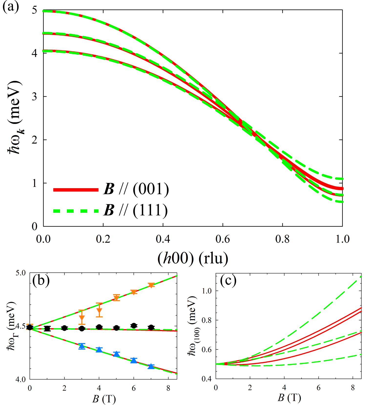
Figure S2: (Color online) a) Dispersion relations along the $(100)$ direction in reciprocal space for a magnetic field $B=8.5$ T applied along (001) (solid red lines) and (111) (dashed green lines), respectively. b) Splitting of excitation energies at the zone center is linear in field and independent of direction, in agreement with experimentally-measured THz transition energies on powder samples (data points from Laurita et al. (2015)). c) In contrast. excitation energies at the softening point (100) show a noticeable dependence on the applied field direction (solid red lines for (001) and dashed green for (111).

Finally we note that the application of a magnetic field leads to a mixing between the zero-field states shown in Fig. S1, inset) with the consequence that transitions become allowed between the ground state $\psi_{0}$ and other higher energy states derived from the $E$-doublet, in addition to transitions to the first three excited states $\psi_{1,2,3}$. Specifically, this mixing allows transitions between the ground state and high energy states originating from the $\Gamma_{3}$ doublet in Fig. S1 (inset). However, the INS data in applied magnetic field shown in Fig. 3 is restricted to the region of low to intermediate energy transfers when only transitions $\psi_{0}\rightarrow\psi_{1,2,3}$ contribute, so the approximations used in deriving the dispersion relations and intensities using the three-flavor pseudo-boson method in Sec. S3 are still expected to be applicable.

VI S5. Background Subtraction using detailed balance

In this section we outline the procedure used to estimate the non-magnetic background contribution to subtract from the measured INS data to obtain the pure magnetic signal. The method uses a measured low-temperature data set, where magnetic signal is expected to be present only on the positive energy side, and a data set measured at relatively high temperatures, in the paramagnetic phase, where a weaker, diffuse, magnetic signal is expected to be present on both the positive and negative energy sides. The relative intensities between the positive and negative energy transfer for a given wavevector transfer $\bm{Q}$ are related by the principle of detailed balance for the dynamical structure factor Squires (1978)

$$S(-\bm{Q},-\hbar\omega)=e^{-\frac{\hbar\omega}{k_{\rm B}T}}S(\bm{Q},\hbar\omega).$$ (S26)

Formally, this is a consequence of the effect of time-reversal on the dynamical structure factor, whereas physically it expresses the fact that the intensity for a given process which transfers energy $\hbar\omega$ to the neutron is exactly the same as for the reverse process (when the neutron transfers energy $\hbar\omega$ to the system) multiplied by a Boltzmann factor. It is seen that in the limit of $T\rightarrow\infty$ both processes are equally likely and contribute symmetrically to the intensity profile. This principle applies regardless of the potential responsible for the scattering. Eq. (S26) implies the same Boltzmann factor relation between the spherically-averaged structure factors $S(Q,\pm\hbar\omega)$, as relevant for a powder INS experiment.

The application of the principle of detailed balance to estimate the non-magnetic background proceeds as follows; at very low temperatures (2.2 K in the experiments outlined in the main text, Fig. S3(a)), the inelastic scattering is concentrated almost entirely on the $\omega>0$ side of the dynamical structure factor profile, as there are very few thermally excited levels within the system able to transfer energy to the neutron. As the temperature increases, the scattering intensity spreads to the $\omega<0$ side as excited states become thermally populated within the system. Assuming that the contribution of magnetic scattering on the $\omega<0$ side (in practice, below the elastic line) is negligible at base temperature, by subtracting this intensity profile from a high temperature data set (in practice, 50 K was found to be high enough, Fig. S3(b)) one can achieve an estimate for the intensity of magnetic scattering processes that transfer energy to the neutron at 50 K, this subtraction is shown in Fig. S3(c). However, (S26) shows that the intensity on the negative $\omega$ side is related to that on the positive $\omega$ side at the same $Q$ via the Boltzmann factor. Thereby, through ‘reflecting’ this negative $\omega$ intensity profile about the elastic line taking account of the Boltzmann factor in (S26), one arrives at an estimate of the high temperature (50 K) magnetic scattering intensity, shown in Fig. S3(d). The ‘reflection’ of the magnetic signal works well for finite energy transfers away from the elastic line, but is not applicable in the very close vicinity of the elastic line where the signals to be subtracted between the two data sets are very large and so extracting small differences is not sufficiently reliable and/or there could be additional scattering contributions with a distinct temperature dependence, see the clear non-smooth behavior very close to the elastic line in Fig. S3(d). In this case we interpolate the paramagnetic scattering intensity in the region covering the close vicinity of the elastic line by assuming a smooth variation of the diffuse scattering signal between the negative and positive energy sides to obtain the plot in Fig. S3(e). This is illustrated in the energy scan in Fig. S3(g). The points below $-1$ meV are from the subtraction 50 K minus 2.2 K data, points above $1.5$ meV are obtained via ‘reflection’, and points in-between are interpolated. The solid line in the figure is a fit to the functional form $I(\omega)=f(\hbar\omega/k_{\rm B}T)G(\omega)$, where $f(x)=x/(1-e^{-x})$ and $G(\omega)$ is a Gaussian of adjustable width centered at $\omega=0$. This parametrization was chosen as i) it satisfies the detailed balance principle in (S26), ii) it converges at $T\rightarrow\infty$ to a smooth profile centered at zero energy, as expected for diffuse paramagnetic scattering, and iii) empirically it appears to be a good parametrization of the observed diffuse scattering, as shown by the comparison in Fig. S3(g). The estimated pure magnetic signal at high temperature in Fig. S3(e) is then subtracted from the raw data in panel (a) to obtain the estimated non-magnetic background plotted in panel (f), this in turn is then subtracted from the low-temperature data in panel (b) to obtain the pure magnetic signal plotted in Fig. 2(a).

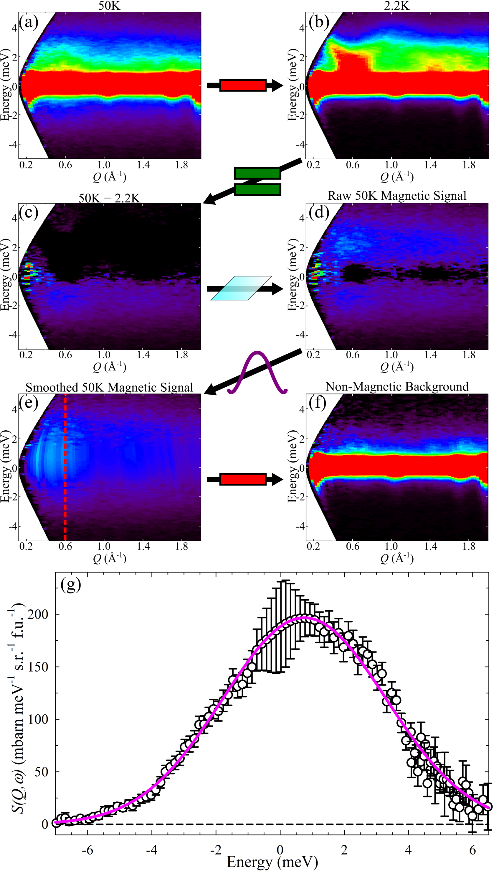
Figure S3: (Color online) Background subtraction procedure: the base temperature (2.2 K) raw data in (b) is subtracted from the high temperature (50 K) raw data in (a) to obtain (c), which contains pure paramagnetic scattering on the negative energy side. The $\omega<0$ data in (c) is then ‘reflected’ onto the $\omega>0$ side using (S26), then interpolated over the elastic line region to obtain the estimated pure paramagnetic scattering in (e), which is then subtracted from the raw data in (a) to obtain the estimated non-magnetic background in (f). (g) Energy scan at $Q=0.6(1)$Å^-1 through the estimated pure magnetic signal at 50 K in (e). Solid line is a fit to an empirical functional form that satisfies the detailed balance relation (S26) and is described in the text. Dashed horizontal line emphasizes that plotted intensities are background subtracted.

VII S6. Powder-averaged Neutron Scattering intensity

The inelastic neutron scattering intensity including polarization and magnetic form factors is Squires (1978)

$$\mkern-144.0muS(\bm{Q},\hbar\omega)=(\gamma r_{0})^{2}f(Q)^{2}\times$$

$$~{}~{}~{}~{}~{}~{}~{}~{}~{}~{}\underset{\alpha,\beta=x,y,z}{\sum}\left(\delta_{\alpha\beta}-\frac{Q_{\alpha}Q_{\beta}}{Q^{2}}\right)S^{\alpha\beta}(\bm{Q},\hbar\omega),$$ (S27)

where $(\gamma r_{0})^{2}=290.6$ mbarns/sr is a conversion factor bringing the intensity into absolute units of mbarns/meV/sr/formula unit, and $f(Q)$ is the magnetic form factor for Fe²⁺ ions. Here $Q_{x,y,z}$, are the components of the wavevector transfer $\bm{Q}$ along the Cartesian $x,y,z$ axes. $S^{\alpha\beta}(\bm{Q},\hbar\omega)$ contain the dynamical correlations for all possible transitions from an initial state, $|i\rangle$ to a final state $|f\rangle$ given by

$$S^{\alpha\beta}(\bm{Q},\hbar\omega) = \sum_{i,f}p_{i}\langle i|L_{\alpha}+2S_{\alpha}|f\rangle\langle f|L_{\beta}+2S_{\beta}|i\rangle\times$$ (S28)

$$\delta(\hbar\omega+E_{i}-E_{f}),$$

where $p_{i}$ is the probability of the system initially being in state $i$, $E_{f}-E_{i}$ is the energy transfer for the $i\rightarrow f$ transitions, and the approximation $g_{S}=2$ has been used. At base temperature only the ground state is populated, $|i\rangle$ then corresponds to the product of $\psi_{0}(\bm{r})$ states at every site $\bm{r}$ in the lattice, and the final states $|f\rangle$ correspond to one-triplon states created by the normal pseudo-boson operators $a^{\prime\dagger}_{\bm{k}}$, $b^{\prime\dagger}_{\bm{k}}$ and $c^{\prime\dagger}_{\bm{k}}$ in (S22), with the dispersion relations $\hbar\omega_{1,2,3}$ given in (S18).

We note that the dynamical correlations for the spin-orbital singlet state have previously been calculated by treating the exchange $J_{2}$ within a random-phase-approximation formalism Chen et al. (2009b). Here we have provided an alternative approach by deriving directly the dispersion relations in the presence of exchange interactions via pseudo-boson triplon operators and deriving explicitly the neutron scattering structure factor (via the transformation to normal triplon operators) for both zero and applied magnetic field.

For zero magnetic field the cross-section (S27) was numerically averaged over a spherical distribution of orientations of $\bm{Q}$ in order to obtain the orientational-averaged intensity as a function of momentum $Q=|\bm{Q}|$ and energy transfer, $S(Q,\hbar\omega)$, and this was directly compared with the measured INS powder data in Fig. 2b). In a finite applied magnetic field the dispersion relations (and neutron cross-section) depend on the applied field direction with respect to the cubic axes (as discussed in Sec. S4), so in this case a more elaborate averaging is required to reflect the fact that the powder contains a spherically-uniform distribution of sample grain orientations with respect to the instrument frame, but all grains have the magnetic field applied along a fixed direction with respect to the instrument frame. Since in the experimental geometry used the (vertical) magnetic field was perpendicular to the (horizontal) scattering plane of the detectors ($\bm{B}\perp\bm{Q}$), the appropriate powder cross-section is obtained by averaging the single-crystal cross-section (S27) over a uniform distribution of wavevectors ${\bm{Q}}$ on a sphere of radius $Q$ and choosing a uniform random direction of the magnetic field in the plane normal to ${\bm{Q}}$. This method was used to calculate the INS spectrum in Figs. 3d-f) and 4a)(dashed lines).

VIII S7. Sample Preparation

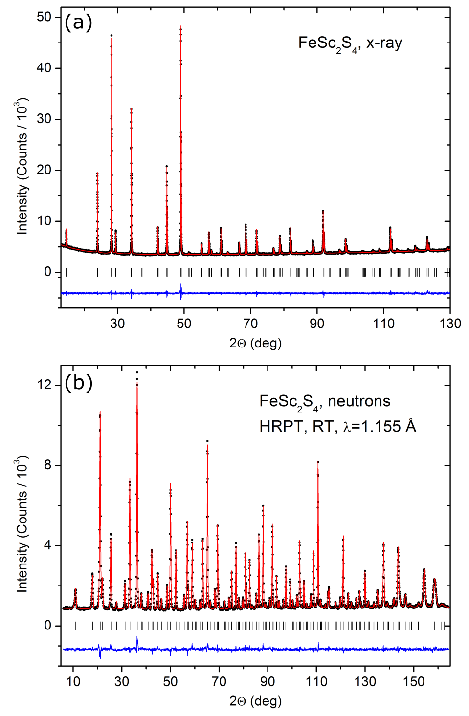
Figure S4: (Color online) Rietveld refinement fit of FeSc₂S₄ crystal structure parameters at room temperature with data from (a) a Bruker D8 powder diffractometer and (b) the HRPT neutron powder diffractometer. Experimental points, calculated profile and the difference curve are shown. The ticks below the graph indicate the calculated positions of the diffraction peaks.

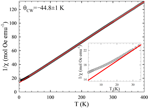
Figure S5: (Color online) Inverse magnetic susceptibility of FeSc₂S₄ powder as a function of temperature (gray circles) in an applied field of $H=10^{4}$ Oe. The thick solid line is a fit to a Curie-Weiss form $\chi=C/(T-\Theta_{\rm CW})$ giving $\Theta_{\rm CW}=-44.8\pm 1$ K. Inset: zoom-in of the low temperature region showing deviation from the linear behavior and the absence of any sharp features indicative of a transition to magnetic order.

Polycrystalline FeSc₂S₄ was prepared by solid state synthesis from the elements: Fe (99.99%), Sc (99.9%), and S (99.999%). Starting materials were loaded into quartz ampoules under Argon atmosphere, then pumped to 10^-2 mbar and closed. After first firing at 900^∘C for 150 h the mixture was reground, pressed into pellets, again closed within an ampoule and fired at the same temperature. To reach full reaction, the sintering procedure was repeated several times (up to 7 cycles). The samples after each cycle were checked by SQUID magnetometry and XRD measurements. To optimize the Fe:Sc:S ratio to the stoichiometric one, additional heat treatments in vacuum and sulfur atmosphere at the last cycles were performed. The composition of the sample was measured by wave-length-dispersive X-ray electron-probe microanalysis (WDS EPMA, Cameca SX50). The data were averaged over points measured on 15 different single-crystalline grains of about 40 $\mu$m in diameter. The obtained composition was Fe 1.006(19) Sc 2.000(33) S 3.977(29) and corresponds to perfect stoichiometry (numbers in the brackets give the standard deviations).

The quality of our powder sample was controlled by x-ray and neutron powder diffraction. The x-ray powder data were collected with a Bruker D8 powder diffractometer (Cu K_α1,2 radiation) in an angular range between 4^∘ and 130^∘ in 2-theta. A profile-matching refinement shown in Fig S4(a) indicates a single phase material with no impurities. Neutron powder diffraction data were collected on the HRPT neutron powder diffractometer Fischer et al. (2000) at room temperature with $\lambda$=1.155 Å neutrons in the angular range 4^∘-165^∘. It confirmed the phase purity of the material and allowed for a precise refinement of its crystal structure parameters. A Rietveld refinement carried out on this same neutron diffraction dataset Fig S4(b) also allowed for the refinement of possible cation disorder over the two cation sites in the structure, i.e. the distribution of the Fe and Sc cations in a compound with a nominal composition FeSc₂S₄ over the 8a(1/8,1/8,1/8) and 16d(1/2,1/2,1/2) sites, to be nominally occupied by solely iron and scandium, respectively. Even though the difference in the bound neutron scattering lengths for Fe and Sc (9.45 and 12.29 fm) is not very large, the relative simplicity of crystal structure in combination with a rather short wavelength – thus covering a sufficiently broad Q-range, up to almost 11 Å^-1 – allows for rather precise refinement results. Given the perfect stochiometry of our sample, we assume iron and scandium are distributed in the ratio 1:2 over these two sites, and the level of disorder is parametrised by $0\leq x\leq 1$ with Fe_1-x Sc_x occupying the 8a, and Sc_2-x Fe_x residing at the 16d sites. The case $x=0(1)$ represents a perfectly uninverted (inverted) structure. The resulting refinement yields a value of x=0.028(8) signifying an extremely low level of inversion. The refined coordinate of sulphur residing in the 32e($\varrho$,$\varrho$,$\varrho$) position is $\varrho$=0.25528(8) which is also quite a typical value for the AB₂O₄ compounds with spinel structures.

Results of magnetic susceptibility measurements (SQUID, MPMS-5, Quantum Design) are shown in Fig. S5 and reveal a linear dependence of the inverse susceptibility on temperature over the range $\approx$ 20-400 K, in agreement with previous reports Fritsch et al. (2004). No evidence for magnetic ordering was found down to the lowest temperature probed, 1.8 K. We note that in contrast to the smooth susceptibility curve in Fig. S5, studies of off-stoichiometry samples of Fe_1.06Sc_1.94S₄ show a clear anomaly at low temperatures as characteristic of the onset of long-range antiferromagnetic order tsu . In contrast, for the powder sample studied here no such anomalies are present. Furthermore $\mu$SR data down to 1.5 K (not shown) indicated only a smooth relaxation without clear oscillations and neutron diffraction could not detect evidence for magnetic Bragg peaks, consistent with the absence of long-range magnetic order in the present samples.

As alluded to in the main text, recently Ref. Plumb et al. (2016) appeared reporting evidence for marginal magnetic order in samples synthesized using a different protocol, suggesting an extreme sensitivity to the synthesis route. We also noted that there are three main physical factors that could lead to such a discrepancy; Vacancies, Site disorder, and Off-stoichiometry. Vacancies at the A-site lead to randomly distributed absences in the diamond lattice of Fe²⁺ ions, thus affecting the finely balanced frustration between NNN sites. Those at the B-site may also lead to a modulation of superexchange interactions as Sulphur ligands are displaced to compensate strains in the structure. However, experiments on samples deliberately synthesised with (up to 5%) vacancies at the Fe sites have been shown to have similar magnetic and thermodynamic properties as those with the ideal crystal structure tsu , suggesting that a small density of such absences is not detrimental. A-B site disorder is a common occurrence in spinels, and with the similar ionic radii of Sc³⁺ and Fe²⁺, great care must be taken in the synthesis of FeSc₂S₄ to minimise such disorder. Off-stoichiometry would also deeply affect the low temperature properties by introducing ionic species other than Fe²⁺, Sc³⁺ and S^2- into the lattice. In particular, for the case of a surplus of Fe, one could presume, for example, the introduction of Fe³⁺ ions into the lattice to preserve charge neutrality. Each of these carry an orbitally non-degenerate $S$=5/2 magnetic moment that could easily order when coupled by exchange interactions to the other magnetic ions in the lattice. To study these effects, we have synthesized samples with deliberate off-stoichiometry (e.g. the Fe_1.06Sc_1.94S₄ mentioned above) and find that those with a surplus of Fe do indeed show very different behaviour from pure FeSc₂S₄. Concretely, magnetic susceptibility measurements on those Fe-rich samples show a deviation between field cooled and zero field cooled data as well as, crucially, the presence of magnetic order at low temperature tsu .

References

- Chen et al. (2009a) G. Chen, L. Balents, and A. P. Schnyder, Phys. Rev. Lett. 102, 096406 (2009a).
- Khaliullin (2013) G. Khaliullin, Phys. Rev. Lett. 111, 197201 (2013).
- Jahn and Teller (1937) H. A. Jahn and E. Teller, Proc. Roy. Soc A: Math. Phys. Eng. Sci. 161, 220 (1937).
- Low and Weger (1960) W. Low and M. Weger, Phys. Rev. 118, 1119 (1960).
- (5) A. Jain, J. Krautloher, M.and Porras, G. H. Ryu, D. P. Chen, D. L. Abernathy, J. T. Park, A. Ivanov, J. Chaloupka, G. Khaliullin, B. Keimer, and B. J. Kim, arXiv:1510.07011 .
- Mittelstädt et al. (2015) L. Mittelstädt, M. Schmidt, Z. Wang, F. Mayr, V. Tsurkan, P. Lunkenheimer, D. Ish, L. Balents, J. Deisenhofer, and A. Loidl, Phys. Rev. B 91, 125112 (2015).
- Fritsch et al. (2004) V. Fritsch, J. Hemberger, N. Büttgen, E.-W. Scheidt, H. A. Krug von Nidda, A. Loidl, and V. Tsurkan, Phys. Rev. Lett. 92, 116401 (2004).
- Krimmel et al. (2005) A. Krimmel, M. Mücksch, V. Tsurkan, M. M. Koza, H. Mutka, and A. Loidl, Phys. Rev. Lett. 94, 237402 (2005).
- Tomas and Guittard (1979) P. A. Tomas and M. Guittard, Matt. Res. Bull. 14, 249 (1979).
- Büttgen et al. (2006) N. Büttgen, A. Zymara, C. Kegler, V. Tsurkan, and A. Loidl, Physical Review B 73, 132409 (2006).
- (11) See Supplemental Material for details of the single ion and spin-orbital triplon calculations, as well as a description of the background subtraction procedure and information on sample preparation and characterization, which includes Refs. Hutchings (1964); Testelin et al. (1992); Grover (1965); White et al. (1965); Maestro and Gingras (2004); Squires (1978); Fischer et al. (2000); tsu .
- Bewley et al. (2006) R. Bewley, R. Eccleston, K. McEwen, S. Hayden, M. Dove, S. Bennington, J. Treadgold, and R. Coleman, Physica B: Condensed Matter 385-386, 1029 (2006).
- Ish and Balents (2015) D. Ish and L. Balents, Phys. Rev. B 92, 094413 (2015).
- Abragam and Bleaney (1970) A. Abragam and B. Bleaney, Electron Paramagnetic Resonance of Transition Ions (Dover, 1970).
- Laurita et al. (2015) N. J. Laurita, J. Deisenhofer, L. D. Pan, C. M. Morris, M. Schmidt, M. Johnsson, V. Tsurkan, A. Loidl, and N. P. Armitage, Phys. Rev. Lett. 114, 207201 (2015).
- not (a) As discussed in Wittekoek et al. (1973); Laurita et al. (2015), the transition from the ground state to the lowest level of the orbital triplet occurs at , where is an energy shift due to the coupling to Jahn-Teller phonons. We have used the estimate meV Laurita et al. (2015) to deduce the energy of the purely electronic transition and this was then used in the data parameterization to constrain and .
- not (b) Note that the usually-assumed lowest order approximation Low and Weger (1960) would predict a value 30% higher than that obtained from directly calculating the energy levels of the full single-ion Hamiltonian.
- Sarkar et al. (2010) S. Sarkar, T. Maitra, R. Valentí, and T. Saha-Dasgupta, Phys. Rev. B 82, 041105 (2010).
- Feiner (1982) L. F. Feiner, Journal of Physics C: Solid State Physics 15, 1515 (1982).
- Chen et al. (2009b) G. Chen, A. P. Schnyder, and L. Balents, Phys. Rev. B 80, 224409 (2009b).
- Rüegg et al. (2008) C. Rüegg, B. Normand, M. Matsumoto, A. Furrer, D. F. McMorrow, K. W. Krämer, H. U. Güdel, S. N. Gvasaliya, H. Mutka, and M. Boehm, Phys. Rev. Lett. 100, 205701 (2008).
- not (c) The -factor characterizing the linear splitting is predicted Ish and Balents (2015) to be wavevector-dependent and vary as the square of the zero-field triplon energy in (2), therefore to become negligibly small near the magnetic softening wavevector, where the regime of linear splitting of the triplet modes is practically unobservable as quadratic and higher order terms in dominate.
- not (d) We have explicitly verified by direct calculation of the wavefunctions that at the single-ion level all the above cases have qualitatively the same behavior in applied field, i.e. the singlet state is stabilized as shown in Fig. 4(b).
- (24) http://dx.doi.org/10.5287/bodleian:KOKPDExm6.
- Plumb et al. (2016) K. W. Plumb, J. R. Morey, J. A. Rodriguez-Rivera, H. Wu, A. A. Podlesnyak, T. M. McQueen, and C. L. Broholm, Phys. Rev. X 6, 041055 (2016).
- Hutchings (1964) M. T. Hutchings, Solid State Phys. 16, 227 (1964).
- Testelin et al. (1992) C. Testelin, C. Rigaux, A. Mauger, A. Mycielski, and C. Julien, Phys. Rev. B 46, 2183 (1992).
- Grover (1965) B. Grover, Phys. Rev. 140, 1944 (1965).
- White et al. (1965) R. M. White, M. Sparks, and I. Ortenburger, Phys. Rev. 139, 450 (1965).
- Maestro and Gingras (2004) A. G. D. Maestro and M. J. P. Gingras, J. Phys. Cond. Matt. 16, 3339 (2004).
- Squires (1978) G. Squires, Introduction to the Theory of Thermal Neutron Scattering (Cambridge University Press, 1978).
- Fischer et al. (2000) P. Fischer, G. Frey, M. Koch, M. Konnecke, V. Pomjakushin, J. Schefer, R. Thut, N. Schlumpf, R. Burge, U. Greuter, S. Bondt, and E. Berruyer, Physica B: Condensed Matter 276-278, 146 (2000).
- (33) V. Tsurkan, A. Loidl et al. (2017) in preparation.
- Wittekoek et al. (1973) S. Wittekoek, R. P. van Stapele, and A. W. J. Wijma, Phys. Rev. B 7, 1667 (1973).