On anisotropy function in crystal growth simulations using Lattice Boltzmann equation

Abstract

In this paper, we present the ability of the Lattice Boltzmann (LB) equation, usually applied to simulate fluid flows, to simulate various shapes of crystals. Crystal growth is modeled with a phase-field model for a pure substance, numerically solved with a LB method in 2D and 3D. This study focuses on the anisotropy function that is responsible for the anisotropic surface tension between the solid phase and the liquid phase. The anisotropy function involves the unit normal vectors of the interface, defined by gradients of phase-field. Those gradients have to be consistent with the underlying lattice of the LB method in order to avoid unwanted effects of numerical anisotropy. Isotropy of the solution is obtained when the directional derivatives method, specific for each lattice, is applied for computing the gradient terms. With the central finite differences method, the phase-field does not match with its rotation and the solution is not any more isotropic. Next, the method is applied to simulate simultaneous growth of several crystals, each of them being defined by its own anisotropy function. Finally, various shapes of 3D crystals are simulated with standard and non standard anisotropy functions which favor growth in $\left\langle 100\right\rangle$-, $\left\langle 110\right\rangle$- and $\left\langle 111\right\rangle$-directions.

1 Introduction

Simulation of crystal growth [1, 2, 3, 4] is a problem of phase change between a solid phase and a liquid phase separated by an interface. Modeling of crystal growth necessitates to follow that interface which is characterized by its surface energy and its kinetic mobility. Those two properties are two anisotropic functions depending on the underlying structure of the crystal.

The phase-field method has become, in recent years, one of the most popular methods for simulating crystal growth and microstructure evolution in materials [1, 2, 4]. In this approach, the geometry of domains and interfaces is described by one or several scalar functions, the phase fields, that take constant values within each domain and vary smoothly but rapidly through the interfaces. The evolution equations for the phase fields, which give the interface dynamics without the need for an explicit front-tracking algorithm, are nonlinear partial differential equations (PDEs) that can be obtained from the principles of out-of-equilibrium thermodynamics. Therefore, they also naturally incorporate thermodynamic boundary conditions at the interfaces, such as the Gibbs-Thomson condition. Moreover, it is straightforward to introduce interfacial anisotropy in phase-field models, which makes it possible to perform accurate simulations of dendritic growth.

In phase-field models, the interfacial energy and the mobility are decomposed into a product of a constant value with a function depending locally on the normal vector of the interface [5, 6, 7, 8, 9, 10, 11, 12, 13, 14, 15, 16, 17, 18, 19]. In the rest of this paper, this function will be called <<anisotropy function>> and will be noted $a_{s}(\mathbf{n})$, where $\mathbf{n}$ is the unit normal vector of the interface. This function is responsible for the characteristic shape of the crystals, it is involved in the phase-field equation. Let us remind that in the <<sharp interface>> formulations [20], the anisotropy function appears in the Gibbs-Thomson condition which gives the interface temperature as a function of the melting temperature, corrected by the curvature and the kinetic mobility of the interface. In the literature, for most of 3D crystal growth simulations, the anisotropy function is chosen such as the branches of crystal grow along the main axes of the coordinate system, i.e. in the $x$-, $y$- and $z$-directions [21, 12, 22, 23, 24]. This particular direction of growth is called the $\left\langle 100\right\rangle$-direction in 3D. Thus, the crystal presents generally a dendritic shape with six tips, two of them being directed along the $x$-axis, two other directed along the $y$-axis and two last ones directed along the $z$-axis.

Phase-field models are composed of highly non-linear PDEs that necessitate to take a special care when discretizing those PDEs, particularly when evaluating the laplacian term in the phase-field equation [12, 25]. Indeed, when a standard finite difference method is used, involving only the first nearest neighbors, a numerical error can occur on the crystal shape: the growth of a sphere has not the spherical shape during the simulation. Such an error is called <<grid anisotropy>> and this problem is fixed by using a finite difference method using eighteen nearest neighbors in 3D [12, 14].

The Lattice Boltzmann (LB) equation is a popular numerical method for simulating fluid flows modeled by Navier-Stokes equations [26, 27, 28]. The method has achieved many successes in problems involving complex fluids, such as two-phase flows [29, 30, 31], flows interacting with a magnetic field [32, 33] and even those that are influenced by crystal growth and solidification [17, 34, 35, 36]. In this method, the main quantity is a distribution function that is moved and performs a collision at each node of a lattice. Macroscopic variables such as density and velocity are calculated at each time step by updating moments of zeroth and first order of this distribution function.

Many works exist in the literature that combine the lattice Boltzmann method with models of solidification or crystal growth [17, 37, 35, 34, 38, 39, 33]. However, in those papers, the LBE is often used to simulate fluid flow, whereas the model of phase change is simulated with another numerical method (e.g. finite difference with an explicit time scheme [37]). In [40, 41], the LB equation was applied to simulate a phase-field model, but the phase-field equation does not correspond to the model solved in this present work ([12]). The main difference is that the anisotropy function $a_{s}(\mathbf{n})$ does not explicitly appear in the models. We propose here to take into account explicitly that anisotropy function by modifying first the standard lattice Boltzmann equation and second the equilibrium distribution function. We will introduce the directional derivatives method to compute accurately that function. On that basis, various anisotropy functions $a_{s}(\mathbf{n})$ will be implemented and simulated in the framework of LB method.

In other examples where the LBE is applied to simulate solidification in presence of interfacial anisotropy, the model used to track the interface between the solid and the liquid is not based on the phase-field theory. For instance in [39], the Gibbs-Thomson condition at the interface is explicitly solved in the numerical procedure, which corresponds to a <<sharp interface>> method. In [42, 35, 38] the model is based on the <<enthalpy-porosity>> approach, an alternative model of solid/liquid phase transition for a pure substance [43, 44]. Finally another class of LB method exists to simulate crystal growth. The method is based on a reaction-diffusion model [45] by applying a first-order kinetic-reaction as boundary conditions at the fluid-solid interface. This method is extended to study dissolution and precipitation in [46, 47]. In that approach, the interface is not explicitly followed by using a PDE and no anisotropy function is involved in the model.

Recently, the lattice Boltzmann schemes were applied on a phase-field model, with or without anti-trapping current, in order to simulate crystal growth of a binary mixture [48, 49]. In those references, numerical methods are well suited for simulating crystal growth with low and moderate Lewis numbers. In more general problems involving high Lewis numbers, the LB numerical schemes have to be modified to take into account a diffusion coefficient which can be ten thousands times smaller than the thermal diffusivity. Nevertheless, the main advantage of this new algorithm lies in its formulation that is identical to the one used in fluid flow. A monolithic code that uses the same distribution functions and same libraries can be used to simulate fluid flow and solidification process. Thank to the same stages of collision and displacement, which can be applied for each equation, a seamless integration with fluid flow simulations could be performed in the future.

In continuation of reference [49], crystal growth is discussed here in terms of anisotropy function $a_{s}(\mathbf{n})$, when the lattice Boltzmann schemes are used for simulations. For simplicity, we focus the presentation on the solidification of a pure substance with the model presented in [12]. Let us emphasize that the methods presented in this paper are also suited for dilute binary mixtures because the anisotropy function is involved only in the phase-field equation. In the LB framework, the grid anisotropy effects on the crystal shape are avoided by using for phase-field equation the lattices D3Q15 or D3Q19 in 3D or D2Q9 in 2D [49]. However, a numerical error may remain if $a_{s}(\mathbf{n})$ is calculated by using the standard method of central finite differences. Indeed, that function necessitates to calculate the interface normal vector $\mathbf{n}$, defined by the gradient of phase-field. Those derivatives must be consistent with the moving directions of underlying lattice in order to avoid additional numerical errors. In this paper, those unwanted numerical errors will be called <<lattice anisotropy>>. The lattice anisotropy occurs especially when the growth of crystal occurs in different directions from the standard $\left\langle 100\right\rangle$ one, e.g. $\left\langle 110\right\rangle$ or $\left\langle 111\right\rangle$.

We show in this work, that the lattice anisotropy can be decreased by using the directional derivatives method [50] for calculating the gradients. Such derivatives are calculated along each direction of propagation on the lattice. The number of directional derivatives is equal to the number of displacement vectors in the LB method. The three gradient components are obtained by calculating their moment of first order. With a standard method of central finite differences, the solution is not isotropic and the phase-field does not match with its rotation. The directional derivatives method has already demonstrated its performance for hydrodynamics problem in order to reduce parasitic currents for two-phase flow problem [51, 52]. Here, we study the impact of the gradient calculation for crystal growth simulations. To the best of authors’ knowledge, the effects of directional derivatives in lattice Boltzmann scheme were not studied for such problems. The entire approach demonstrates the ability of the LB equation for simulating various shapes of crystal in 2D and 3D.

This paper is organized as follows. Section 2 will present the mathematical model for crystal growth based on the phase-field theory. Next, Section 3 will present the lattice Boltzmann methods that we used to simulate the phase-field model. Section 4 will remind the main formulations of anisotropy function $a_{s}(\mathbf{n})$, which can be defined either with the local angle $\varphi$ (between $\mathbf{n}$ and the $x$-axis) in 2D, or by using the components of normal vector $\mathbf{n}=(n_{x},\,n_{y},\,n_{z})^{T}$ in 3D. A comparison between the directional derivatives method and the finite differences method will be presented in this section. That section will also present simulations on simultaneous growth of several crystals, each of them being defined by its own anisotropy function. Finally, section 5 will present 3D simulations of various crystals shapes obtained with standard and non standard anisotropy functions which favor the growth in directions $\left\langle 100\right\rangle$, $\left\langle 110\right\rangle$ and $\left\langle 111\right\rangle$.

2 Phase-field model for a pure substance

In this work, we focus on the solidification of a pure substance. For such a problem, the main physical process is the heat diffusion in solid and liquid. The heat fluxes are modeled by the Fourier’s law and we assume for simplicity that properties such as specific heat $C_{p}$ and thermal diffusivity $\kappa$ are constant and identical in each phase. The solidification can be modeled by heat equation applied in the bulk phases with two additional equations at the interface. The first one is the energy conservation and the second one is the Gibbs-Thomson condition. During the solidification, the velocity of the interface multiplied by the latent heat $L$, released into the liquid, is balanced with the difference between the heat fluxes in the solid and the liquid. For the second interfacial boundary condition, the Gibbs-Thomson condition gives the interfacial temperature as a function of the melting temperature $T_{m}$ corrected by the curvature and the mobility of the interface. The mathematical equations of that <<sharp interface>> model can be found in many references such as [12, 53, 14, 2].

In phase-field theory, the interfacial boundary conditions are replaced by the phase-field equation. The interface position is given by a continuous function $\phi\equiv\phi(\mathbf{x},\,t)$, the phase-field (dimensionless), defined over the whole computational domain. The interface is now a diffuse one with an interface thickness noted $W_{0}$. In our work we assume that $\phi=-1$ and $\phi=+1$ correspond respectively to the liquid phase and the solid phase. The model is thermodynamically consistent, i.e. it is derived by postulating a free energy functional depending upon a double-well potential plus a gradient term [21, 11, 12]. The model is composed of two PDEs, the first one for the phase-field $\phi$ and the second one for the normalized temperature $u\equiv u(\mathbf{x},\,t)$ (dimensionless) defined by $u(\mathbf{x},\,t)=C_{p}(T(\mathbf{x},\,t)-T_{m})/L$:

$$\tau(\mathbf{n})\frac{\partial\phi}{\partial t} =W_{0}^{2}\boldsymbol{\nabla}\cdot(a_{s}^{2}(\mathbf{n})\boldsymbol{\nabla}\phi)+W_{0}^{2}\boldsymbol{\nabla}\cdot\boldsymbol{\mathcal{N}}+(\phi-\phi^{3})-\lambda u(1-\phi^{2})^{2},$$ (1a)

$$\frac{\partial u}{\partial t} =\kappa\boldsymbol{\nabla}^{2}u+\frac{1}{2}\frac{\partial\phi}{\partial t},$$ (1b)

where $\boldsymbol{\mathcal{N}}\equiv\boldsymbol{\mathcal{N}}(\mathbf{x},\,t)$ is defined by:

$$\boldsymbol{\mathcal{N}}(\mathbf{x},\,t)=\bigl{|}\boldsymbol{\nabla}\phi\bigr{|}^{2}a_{s}(\mathbf{n})\left(\frac{\partial a_{s}(\mathbf{n})}{\partial(\partial_{x}\phi)},\,\frac{\partial a_{s}(\mathbf{n})}{\partial(\partial_{y}\phi)},\,\frac{\partial a_{s}(\mathbf{n})}{\partial(\partial_{z}\phi)}\right)^{T}.$$ (1c)

The anisotropy function $a_{s}(\mathbf{n})$ (dimensionless) for a growing direction $\left\langle 100\right\rangle$ is:

$$a_{s}(\mathbf{n})=1-3\varepsilon_{s}+4\varepsilon_{s}\sum_{\alpha=x,y,z}n_{\alpha}^{4}.$$ (1d)

In Eq. (1a), $\phi$ is the phase-field, $W_{0}$ is the interface thickness, $\lambda$ is the coupling coefficient with the normalized temperature $u(\mathbf{x},\,t)$. The normal vector $\mathbf{n}\equiv\mathbf{n}(\mathbf{x},\,t)$ is defined such as:

$$\mathbf{n}(\mathbf{x},\,t)=-\frac{\boldsymbol{\nabla}\phi}{\bigl{|}\boldsymbol{\nabla}\phi\bigr{|}},$$ (1e)

directed from the solid to the liquid. The coefficient $\tau(\mathbf{n})$ is the kinetic coefficient of the interface, it is defined as $\tau(\mathbf{n})=\tau_{0}a_{s}^{2}(\mathbf{n})$ where $\tau_{0}$ is the kinetic characteristic time. Let us notice that each term of Eq. (1a) is dimensionless. The physical dimensions of $W_{0}$, $\boldsymbol{\mathcal{N}}$, $\tau_{0}$ and $\lambda$ are respectively $[W_{0}]\equiv[\mathscr{L}]$, $[\boldsymbol{\mathcal{N}}]\equiv[\mathscr{L}]^{-1}$, $[\tau_{0}]\equiv[\mathcal{T}]$ and $[\lambda]\equiv[-]$, where $[\mathscr{L}]$ indicates the length dimension and $[\mathcal{T}]$ indicates the time dimension. In Eq. (1b), the physical dimension of $\kappa$ is $[\mathscr{L}]^{2}/[\mathcal{T}]$.

In phase-field models, the capillary effects can be simulated by defining the interface thickness as a function depending on the normal vector of the interface $\mathbf{n}$. In other words, the definition $W(\mathbf{n})=W_{0}a_{s}(\mathbf{n})$ where $a_{s}(\mathbf{n})$ is the anisotropy function of the interfacial energy allows to simulate correctly the growth of crystal with anisotropic shapes. In the model, the second term in the right-hand side of Eq. (1a) is responsible for such a dendritic structure. The term $(\phi-\phi^{3})$ is the derivative of the double-well potential and the last term $\lambda u(1-\phi^{2})^{2}$ is the coupling term with the normalized temperature, interpolated in the diffuse interface. Heat equation (Eq. (1b)) is a standard diffusive equation with a source term involving the time derivative of phase-field: $(1/2)\partial\phi/\partial t$. The meaning of this term can be understood by multiplying Eq. (1b) by the latent heat $L$ which is involved in the definition of $u$. That term models the release of latent heat during the solidification process.

The phase-field equation Eq. (1a) involves three parameters $W_{0}$, $\tau_{0}$ and $\lambda$. Matched asymptotic expansions provide relationships between those parameters with the capillary length $d_{0}$ and the interface kinetic coefficient $\beta$ of the sharp-interface model [12]:

$$d_{0} =a_{1}\frac{W_{0}}{\lambda},$$ (2a)

$$\beta =a_{1}\left(\frac{\tau_{0}}{W_{0}\lambda}-a_{2}\frac{W_{0}}{\kappa}\right).$$ (2b)

Coefficients $a_{1}$ and $a_{2}$ are two numbers of order unity: $a_{1}=5\sqrt{2}/8$, and $a_{2}\approx 0.6267$. These relations make it possible to choose phase-field parameters for prescribed values of the capillary length (surface energy) and the interface mobility (interface kinetic coefficient). Eqs. (2a) and (2b) will be applied in Section 4 for simulating a crystal which grows without kinetic coefficient ($\beta=0$).

Note that the interface width $W_{0}$ is a parameter that can be freely chosen in this formulation; the asymptotic analysis remains valid as long as $W_{0}$ remains much smaller than any length scale present in the sharp-interface solution of the considered problem (for example, a dendrite tip radius in the case of dendritic growth). More details about the dependence of parameters with $\mathbf{n}$ and the link of the phase-field model with the sharp interface model can be found in [14]. That model of crystal growth was applied in many references [25, 14, 54, 23] and serves as basis for model of dilute binary mixture [16, 24] and model of coupling with fluid flows [55, 17, 22].

The characteristic shape of the crystal is obtained by defining appropriately the $a_{s}(\mathbf{n})$ function. If the growing direction $\left\langle 100\right\rangle$ is considered, this function is defined by Eq. (1d). In this relationship, $\varepsilon_{s}$ is the strength of anisotropy and $n_{\alpha}$ ($\alpha=x,\,y,\,z$) is the $\alpha$-component of $\mathbf{n}$. The choice of function (1d) yields to a dendritic shape which presents four tips in 2D and six tips in 3D [11, 21]. In this paper, we focus on the way to simulate crystal growth with various anisotropy functions $a_{s}(\mathbf{n})$ by using the LB method.

For all simulations in this paper, the computational domain is a square in 2D or a cube in 3D, and zero fluxes are imposed on all boundaries for both equations. For phase-field equation, a nucleus is initialized as a diffuse sphere:

$$\phi(\mathbf{x},\,0)=\tanh\left[\frac{R_{s}-d_{s}}{\sqrt{2W{}_{0}}}\right],$$ (3)

where $R_{s}$ is the radius, $d_{s}$ is the distance defined by $d_{s}=[(x-x_{s})^{2}+(y-y_{s})^{2}+(z-z_{s})^{2}]^{1/2}$ and $\mathbf{x}_{s}=(x_{s},\,y_{s},\,z_{s})^{T}$ is the position of its center. With this initial condition, $\phi=+1$ inside the sphere (solid) and $\phi=-1$ outside (liquid). The initial temperature is considered as a constant on the whole domain and fixed below the melting temperature: $T<T_{m}$. The initial condition of the normalized temperature is set such as:

$$u(\mathbf{x},\,0)=u_{0}<0.$$ (4)

In the following simulations, the undercooling defined by $\Delta=-u_{0}$ will be specified.

3 Lattice Boltzmann schemes

LB methods are usually applied to simulate fluid flows. Here, the standard LB equation with the classical equilibrium distribution function (e.d.f.) have to be modified for simulating Eqs. (1a)–(1e). Indeed, fluid flows model involves one scalar equation (mass balance) plus one vectorial equation (momentum) whereas the phase-field model is composed of two scalar equations which are coupled and non-linear. LB methods for phase-field model of crystal growth are already presented in details in reference [49]. They were applied on a model of dilute binary mixture with anti-trapping current which is an extension of a pure substance model. Following that reference, LB schemes are described here for heat equation and phase-field equation. The heat equation is a standard diffusion equation with a particular source term. For a pedagogical presentation, we start the description of algorithms with that equation, because the classical LB method for a diffusive equation is applied (e.g. [56]). Modifications that have to be done for the phase-field equation will be presented and commented in subsection 3.2.

3.1 Heat equation

The LB method works on a distribution function $f_{i}(\mathbf{x},\,t)$ depending on position $\mathbf{x}$ and time $t$. The index $i$ identifies the moving directions on a lattice: $i=0,\,...,\,N_{pop}$ where $N_{pop}$ is the total number of directions. The lattice choice (space dimension and number of moving directions) depends on the physical problem to be simulated. The lattices used in this work are presented in subsection 3.3. The heat equation (1b) is a diffusion equation with a source term involving the time derivative of $\phi$. For that equation, the standard LB equation with the Bhatnagar-Gross-Krook (BGK) approximation for the collision term is applied:

$$f_{i}(\mathbf{x}+\mathbf{e}_{i}\delta x,\,t+\delta t)=f_{i}(\mathbf{x},\,t)-\frac{1}{\eta_{u}}\left[f_{i}(\mathbf{x},\,t)-f_{i}^{(0)}(\mathbf{x},\,t)\right]+w_{i}Q_{u}(\mathbf{x},\,t)\delta t.$$ (5a)

Note that the LB equation (Eq. (5a)) is an evolution equation for $f_{i}(\mathbf{x},\,t)$ which is already discretized in space, time, and moving directions. The space-step is noted $\delta x$ by assuming $\delta x=\delta y=\delta z$ and the time-step is noted $\delta t$. Vectors of displacement on the lattice are noted $\mathbf{e}_{i}$ and $w_{i}$ are weights. The quantities $N_{pop}$, $\mathbf{e}_{i}$ and $w_{i}$ are lattice-dependent and will be specified in table 1 of subsection 3.3. In Eq. (5a), the BGK collision term is the second term in the right-hand side. It relaxes the distribution function $f_{i}(\mathbf{x},\,t)$ toward an equilibrium distribution function (e.d.f.) $f_{i}^{(0)}(\mathbf{x},\,t)$ with a relaxation rate $\eta_{u}$. In such an equation, $f_{i}(\mathbf{x},\,t)$ can be regarded as an intermediate function introduced to calculate the normalized temperature $u(\mathbf{x},\,t)$ and updated at each time step by:

$$u(\mathbf{x},\,t)=\sum_{i=0}^{N_{pop}}f_{i}(\mathbf{x},\,t).$$ (5b)

Eq. (5b) is called the moment of zeroth order of the distribution function $f_{i}$. Moments of first and second order are defined respectively by $\sum_{i=0}^{N_{pop}}f_{i}\mathbf{e}_{i}$ (vector) and $\sum_{i=0}^{N_{pop}}f_{i}\mathbf{e}_{i}\mathbf{e}_{i}$ (tensor of second order). In Eq. (5a), the equilibrium distribution function $f_{i}^{(0)}(\mathbf{x},\,t)$ and the source term $Q_{u}(\mathbf{x},\,t)$ are given by:

$$f_{i}^{(0)}(\mathbf{x},\,t) =w_{i}u(\mathbf{x},\,t),$$ (5c)

$$Q_{u}(\mathbf{x},\,t) =\frac{1}{2}\frac{\partial\phi}{\partial t}.$$ (5d)

By carrying out the Chapman-Enskog’s expansions of Eq. (5a) with Eq. (5c), the first- and second-order moments of the equilibrium distribution function are equal to $\sum_{i}f_{i}^{(0)}\mathbf{e}_{i}=\mathbf{0}$ and $\sum_{i}f_{i}^{(0)}\mathbf{e}_{i}\mathbf{e}_{i}=u(\mathbf{x},\,t)e^{2}\overline{\overline{\mathbf{I}}}$, where $\overline{\overline{\mathbf{I}}}$ is the identity tensor of rank 2. An additional lattice-dependent coefficient, $e^{2}$, arises from the second-order moment of $f_{i}^{(0)}$. Values of $e^{2}$ are given in table 1 for four lattices used in this work. The thermal diffusivity $\kappa$ is related to the relaxation rate of collision $\eta_{u}$ by:

$$\kappa=e^{2}\left(\eta_{u}-\frac{1}{2}\right)\frac{\delta x^{2}}{\delta t}.$$ (5e)

The index $u$ in $Q_{u}$ and $\eta_{u}$ indicates that both quantities are relative to the heat equation. Note that the relaxation rate $\eta_{u}$ is a constant because the thermal diffusivity $\kappa$ was assumed constant in the model. Being given $\kappa$, $\delta x$ and $\delta t$, the relaxation parameter is initialized before the time loop and kept constant during the simulation. In a more general case, $\kappa$ can be a function depending on space and time. In that case, the relationship (5e) must be inverted and the relaxation parameter has to be updated at each time step. Let us notice that the factor $\delta x^{2}/\delta t$ in the right-hand side is homogeneous to $[\mathscr{L}]^{2}/[\mathcal{T}]$, which is consistent with the physical dimension of $\kappa$.

The principle of the LB scheme is the following. Once the normalized temperature $u$ is known with the initial condition, the equilibrium distribution function $f_{i}^{(0)}$ is computed by using Eq. (5c). The collision stage (right-hand side of Eq. (5a)) is next calculated and yields an intermediate distribution function that will be streamed in each direction (left-hand side of Eq. (5a)). Finally after updating the boundary conditions, the new temperature is calculated by using Eq. (5b) and the algorithm is iterated in time.

Notice that the collision term is local and the scheme is fully explicit, i.e., all terms in the right-hand side of Eq. (5a) are defined at position $\mathbf{x}$ and time $t$. Also note that the source term $Q_{u}$ involves the time derivative of the phase field which is approximated here by an explicit Euler scheme: $\partial\phi/\partial t\cong(\phi(\mathbf{x},\,t)-\phi(\mathbf{x},\,t-\delta t))/\delta t$. In practice, the heat equation must be solved after solving the phase-field equation. At the first time-step, the derivative is obtained by the difference between the phase-field at the first time-step and its initial condition.

Finally, this scheme can be easily extended to simulate the Advection-Diffusion Equation (ADE) (e.g. [57]): $\partial u/\partial t=\kappa\boldsymbol{\nabla}^{2}u-\boldsymbol{\nabla}\cdot(u\mathbf{v})$, where $\mathbf{v}$ is the advective velocity, by modifying the equilibrium distribution function such as $f_{i}^{(0)\,ADE}=w_{i}u\left[1+e^{-2}\mathbf{e}_{i}\cdot\mathbf{v}\delta t/\delta x\right]$. Moments of zeroth-, first- and second-order of $f_{i}^{(0)\,ADE}$ are respectively $u$, $\mathbf{v}u\delta t/\delta x$ and $e^{2}u\overline{\overline{\mathbf{I}}}$. In next subsection, the LB method for the phase-field equation is presented with an analogy with this ADE.

3.2 Phase-Field equation

Phase-field equation (Eq. (1a)) looks like an ADE with two differences. The first one is the presence of an additional factor $\tau(\mathbf{n})=\tau_{0}a_{s}^{2}(\mathbf{n})$ in front of the time derivative $\partial\phi/\partial t$ in the left-hand side. The second difference is the presence of the divergence term $W_{0}^{2}\boldsymbol{\nabla}\cdot\boldsymbol{\mathcal{N}}$ in the right-hand side, which is not strictly speaking one <<advective>> term. In order to handle those two terms, the standard LB scheme has to be modified. First, a new distribution function $g_{i}(\mathbf{x},\,t)$ is introduced. The LBE for the phase-field equation works on that function. The first difference necessitates a modification of the evolution equation for $g_{i}$. The second difference requires a modification of the equilibrium distribution function $g_{i}^{(0)}(\mathbf{x},\,t)$.

The numerical scheme is:

$$a_{s}^{2}(\mathbf{n})g_{i}(\mathbf{x}+\mathbf{e}_{i}\delta x,\,t+\delta t)=g_{i}(\mathbf{x},\,t)-(1-a_{s}^{2}(\mathbf{n}))g_{i}(\mathbf{x}+\mathbf{e}_{i}\delta x,\,t)-\frac{1}{\eta_{\phi}(\mathbf{x},\,t)}\left[g_{i}(\mathbf{x},\,t)-g_{i}^{(0)}(\mathbf{x},\,t)\right]+w_{i}Q_{\phi}(\mathbf{x},\,t)\frac{\delta t}{\tau_{0}},$$ (6a)

with the equilibrium distribution function $g_{i}^{(0)}(\mathbf{x},\,t)$ defined by:

$$g_{i}^{(0)}(\mathbf{x},\,t)=w_{i}\left(\phi(\mathbf{x},\,t)-\frac{1}{e^{2}}\mathbf{e}_{i}\cdot\boldsymbol{\mathcal{N}}(\mathbf{x},\,t)\frac{\delta t}{\delta x}\frac{W_{0}^{2}}{\tau_{0}}\right).$$ (6b)

In Eq. (6a), the anisotropy function $a_{s}(\mathbf{n})$ has to be specified. It is defined by Eq. (1d) for simulating one crystal that grows in a preferential direction $\left\langle 100\right\rangle$. In order to simulate other preferential directions of growth, a modification of that function is necessary. Analytic expressions of various anisotropy functions will be specified in Section 4.1. Whatever the relationship used, calculation of $a_{s}(\mathbf{n})$ requires the computation of $\mathbf{n}$ which is defined by the gradient of phase-field $\boldsymbol{\nabla}\phi$. The calculation of that gradient will be presented in Section 4.2. In Eq. (6b), the vector $\boldsymbol{\mathcal{N}}(\mathbf{x},\,t)$ is defined by Eq. (1c). Once the anisotropy function $a_{s}(\mathbf{n})$ is set, the components of $\boldsymbol{\mathcal{N}}$ are calculated by deriving $a_{s}(\mathbf{n})$ with respect to $\partial_{x}\phi$, $\partial_{y}\phi$ and $\partial_{z}\phi$. In Eqs. (6a)–(6b), functions $a_{s}(\mathbf{n})$ and $\boldsymbol{\mathcal{N}}(\mathbf{x},\,t)$ are treated explicitly in time.

The lattice Boltzmann scheme for the phase-field equation differs from the standard LB method for ADE on two points. The first difference is the presence in Eq. (6a) of (i) a factor $a_{s}^{2}(\mathbf{n})$ in front of $g_{i}(\mathbf{x}+\mathbf{e}_{i}\delta x,\,t+\delta t)$ in the left-hand side and (ii) an additional term $(1-a_{s}^{2}(\mathbf{n}))g_{i}(\mathbf{x}+\mathbf{e}_{i}\delta x,\,t)$ in the right-hand side. The latter term is non-local in space, i.e., it is involved in the collision step at time $t$ and needs the knowledge of $g_{i}$ at the neighboring nodes $\mathbf{x}+\mathbf{e}_{i}\delta x$. Those two terms appear to handle the factor $a_{s}^{2}(\mathbf{n})$ in front of the time derivative $\partial\phi/\partial t$ in Eq. (1a). It is straightforward to prove it by carrying out the Taylor’s expansion of Eq. (6a).

The second difference with the LB algorithm for ADE, is the definition of the equilibrium distribution function $g_{i}^{(0)}$ (Eq. (6b)). Moments of zeroth-, first- and second-order of this function are respectively:

$$\sum_{i=0}^{N_{pop}}g_{i}^{(0)}(\mathbf{x},\,t) =\phi(\mathbf{x},\,t)$$ (7a)

$$\sum_{i=0}^{N_{pop}}g_{i}^{(0)}(\mathbf{x},\,t)\mathbf{e}_{i} =-\boldsymbol{\mathcal{N}}(\mathbf{x},\,t)\frac{\delta t}{\delta x}\frac{W_{0}^{2}}{\tau_{0}}$$ (7b)

$$\sum_{i=0}^{N_{pop}}g_{i}^{(0)}(\mathbf{x},\,t)\mathbf{e}_{i}\mathbf{e}_{i} =\phi(\mathbf{x},\,t)e^{2}\overline{\overline{\mathbf{I}}}$$ (7c)

where $\overline{\overline{\mathbf{I}}}$ is still the identity tensor of rank 2. The main difference with the e.d.f. of ADE appears in the moment of first order (Eq. (7b)). In that term, the scalar field $\phi(\mathbf{x},\,t)$ is not involved in the right-hand side because it does not appear in the divergence term of Eq. (1a). The absence of phase field $\phi(\mathbf{x},\,t)$ in the divergence term, explains its presence in the first term inside the brackets (6b), and not before the brackets. Moreover, note the sign change in front of the scalar product $\mathbf{e}_{i}\cdot\boldsymbol{\mathcal{N}}$, which corresponds to the sign change of $+\boldsymbol{\nabla}\cdot\boldsymbol{\mathcal{N}}$ compared to $-\boldsymbol{\nabla}\cdot(\mathbf{v}u)$ for the ADE. A dimensional analysis shows that Eqs. (6a) and (6b) are both dimensionless. In the e.d.f., the second term in the brackets is dimensionless since $[\boldsymbol{\mathcal{N}}]\equiv[\mathscr{L}]^{-1}$, $[W_{0}]\equiv[\mathscr{L}]$ and $[\tau_{0}]\equiv[\mathcal{T}]$.

The algorithm works in the same way than the previous one for the temperature field $u(\mathbf{x},\,t)$. After the collision stage and the streaming step, the phase-field $\phi(\mathbf{x},\,t)$ is calculated by the moment of zeroth order:

$$\phi(\mathbf{x},\,t)=\sum_{i=0}^{N_{pop}}g_{i}(\mathbf{x},\,t).$$ (8a)

The scalar function $Q_{\phi}(\mathbf{x},\,t)$ is the source term of the phase-field equation (1a) which is defined by:

$$Q_{\phi}(\mathbf{x},\,t) =\left[\phi-\lambda u(1-\phi^{2})\right](1-\phi^{2}).$$ (8b)

In Eq. (1a), coefficient $a_{s}^{2}(\mathbf{n})$ in the first term of the right-hand side plays a similar role as a <<diffusion>> coefficient depending on position and time (through $\mathbf{n}$ that depends on $\phi$). The relaxation rate $\eta_{\phi}(\mathbf{x},\,t)$ is a function of position and time and must be updated at each time step by the relationship:

$$\eta_{\phi}(\mathbf{x},\,t)=\frac{1}{e^{2}}a_{s}^{2}(\mathbf{n})\frac{W_{0}^{2}}{\tau_{0}}\frac{\delta t}{\delta x^{2}}+\frac{1}{2}.$$ (8c)

In Eq. (8c), we can check that the first term of the right-hand side is dimensionless: $W_{0}^{2}/\tau_{0}$ is dimensionally balanced with $\delta t/\delta x^{2}$. The origin of factor $W_{0}^{2}/\tau_{0}$ inside $g_{i}^{(0)}$ (Eq. (6b)) and $\eta_{\phi}$ (Eq. (8c)), can be understood by dividing each term of Eq. (1a) by $\tau_{0}$. The first term in the right-hand side becomes $\boldsymbol{\nabla}\cdot\left[(a_{s}^{2}(\mathbf{n})W_{0}^{2}/\tau_{0})\boldsymbol{\nabla}\phi\right]$, the second one becomes $\boldsymbol{\nabla}\cdot(\boldsymbol{\mathcal{N}}W_{0}^{2}/\tau_{0})$ and the last one is $Q_{\phi}/\tau_{0}$. Each term $(a_{s}^{2}(\mathbf{n})W_{0}^{2}/\tau_{0})$, $(\boldsymbol{\mathcal{N}}W_{0}^{2}/\tau_{0})$ and $Q_{\phi}/\tau_{0}$ is respectively involved in Eqs. (8c), (6b) and (6a). More rigorously, after the asymptotic expansions of Eq. (6a), the moments equation for $g_{i}^{(0)}$ is compared to Eq. (1a) divided by $\tau_{0}$. The identification of each term yields to the relationships (7a)–(7c) and (8c). The Chapman-Enskog’s expansions of that numerical scheme can be found in Appendices of reference [49].

The LB scheme for phase-field equation uses the same BGK collision rule than temperature equation. Other approximations of the collision term exist in the literature: Multiple-Relaxation Time (MRT) [58] and Two-Relaxation Time (TRT) [59]. With the MRT approximation the collisions are carried out in the moments space. For ADE, tensorial diffusion coefficients can be taken into account for problems that involve diffusion coefficients varying with direction [60]. Moreover, with the MRT and TRT approximations, it is possible to simulate problems with higher Peclet numbers than those reached with the BGK collision. High Peclet number and anisotropic diffusion coefficient are not studied here.

3.3 Lattices

Several lattices exist in the LB method, they differ by the space dimension and the number of moving directions. In this work, 2D and 3D simulations are carried out with four lattices: D2Q5, D2Q9, D3Q7 and D3Q15 (see Fig. 1). The lattices D2Q5 and D2Q9 are applied for two-dimensional simulations (D2) and uses respectively five (Q5) and nine (Q9) directions of displacement. The lattice D2Q5 is applied for temperature equation and D2Q9 for phase-field equation. For three-dimensional simulations, the temperature $u$ is computed on a lattice D3Q7, whereas the phase-field $\phi$ is computed on a lattice D3Q15. The first one is defined by seven directions of displacement (Q7) and the second one is defined by fifteen directions (Q15). The displacement vectors $\mathbf{e}_{i}$ are defined below for each lattice.

(a) D2Q5		(b) D2Q9
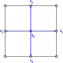
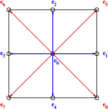
(c) D3Q7		(d) D3Q15

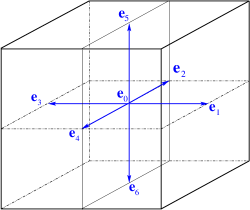
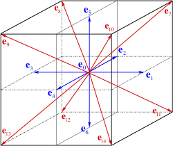
Figure 1: (a) Two-dimensional simulations: lattices (a) D2Q5 for temperature equation and (b) D2Q9 for phase-field equation. Three-dimensional simulations: (c) D3Q7 for temperature equation and (d) D3Q15 for phase-field equation.

Lattices	Weights
2D $N_{pop}$ $e^{2}$ D2Q5 $4$ $1/3$ D2Q9 $8$ $1/3$ 3D $N_{pop}$ $e^{2}$ D3Q7 $6$ $1/4$ D3Q15 $14$ $1/3$	$w_{0}$ $w_{1,...,4}$ $w_{5,...,8}$ $1/3$ $1/6$ $-$ $4/9$ $1/9$ $1/36$ $w_{0}$ $w_{1,...,6}$ $w_{7,...,14}$ $1/4$ $1/8$ $-$ $2/9$ $1/9$ $1/72$

Table 1: Values of $N_{pop}$, $w_{i}$, and $e^{2}$ for lattices D2Q5, D2Q9, D3Q7 and D3Q15.

Although the phase-field equation (Eq. (1a)) is a scalar one, the simplest lattices such as D2Q5 and D3Q7 are avoided. Indeed, some unwanted effects of grid anisotropy can occur by using them. For instance, the choice $\varepsilon_{s}=0$ in Eq. (1d) does not yield to a solution with a spherical shape (see [49]). Let us mention that the same problem occurs when the laplacian term of phase-field equation is discretized with a finite difference method which uses only the first four (in 2D) or six (in 3D) neighbors [12]. That problem is fixed by using eighteen neighboring nodes in 3D simulations [14]. At last, the lattices D3Q19 and D3Q27 are not applied because the same solution as D3Q15 is obtained by using them. Those two lattices use more moving directions and require more memory.

The two-dimensional lattices D2Q5 and D2Q9 are defined as follows. The number of moving directions are respectively $N_{pop}=4$ and $N_{pop}=8$. For D2Q5, vectors $\mathbf{e}_{i}$ are defined by $\mathbf{e}_{0}=(0,\,0)^{T}$, $\mathbf{e}_{1}=(1,\,0)^{T}$, $\mathbf{e}_{2}=(0,\,1)^{T}$, $\mathbf{e}_{3}=(-1,\,0)^{T}$ and $\mathbf{e}_{4}=(0,\,-1)^{T}$ (Fig. 1a). For D2Q9 the first five vectors are the same (blue vectors on Fig. 1b) and the last four vectors correspond to the four diagonals of the square (red vectors on Fig. 1b): $\mathbf{e}_{5}=(1,\,1)^{T}$, $\mathbf{e}_{6}=(-1,\,1)^{T}$, $\mathbf{e}_{7}=(-1,\,-1)^{T}$, $\mathbf{e}_{8}=(1,\,-1)^{T}$.

For D3Q7, the number of moving directions is $N_{pop}=6$. Vectors $\mathbf{e}_{i}$ are defined such as $\mathbf{e}_{0}=(0,\,0,\,0)^{T}$, $\mathbf{e}_{1}=(1,\,0,\,0)^{T}$, $\mathbf{e}_{2}=(0,\,1,\,0)^{T}$, $\mathbf{e}_{3}=(-1,\,0,\,0)^{T}$, $\mathbf{e}_{4}=(0,\,-1,\,0)^{T}$, $\mathbf{e}_{5}=(0,\,0,\,1)^{T}$ and $\mathbf{e}_{6}=(0,\,0,\,-1)^{T}$ (Fig. 1c). For D3Q15, the number of moving directions is $N_{pop}=14$. The first seven vectors $\mathbf{e}_{i}$ are the same as D3Q7 (blue vectors on Fig. 1d). The eight other directions correspond to the eight diagonals of the cube (red vectors on Fig. 1d) and are defined by: $\mathbf{e}_{7}=(1,\,1,\,1)^{T}$, $\mathbf{e}_{8}=(-1,\,1,\,1)^{T}$, $\mathbf{e}_{9}=(-1,\,-1,\,1)^{T}$, $\mathbf{e}_{10}=(1,\,-1,\,1)^{T}$, $\mathbf{e}_{11}=(1,\,1,\,-1)^{T}$, $\mathbf{e}_{12}=(-1,\,1,\,-1)^{T}$, $\mathbf{e}_{13}=(-1,\,-1,\,-1)^{T}$, $\mathbf{e}_{14}=(1,\,-1,\,-1)^{T}$ .

Finally, values of $e^{2}$ and $w_{i}$ for those four lattices are given in Table 1. All quantities are calculated at nodes and the weights $w_{i}$ are defined such as $\sum_{i=1,...,N_{pop}}w_{i}=1$. As usual in LB method, the condition $\delta x=\delta y=\delta z$ is assumed: meshes are squares (in 2D) or cubes (in 3D). In this work, for all boundaries of computational domain, the standard bounce-back method is applied for both distribution functions $f_{i}$ and $g_{i}$:

$$f_{i}(\mathbf{x},\,t) =f_{i^{\prime}}(\mathbf{x},\,t),$$ (9a)

$$g_{i}(\mathbf{x},\,t) =g_{i^{\prime}}(\mathbf{x},\,t),$$ (9b)

where $i^{\prime}$ is the opposite direction of $i$. For instance, for temperature equation, after the streaming step, components $f_{1}$, $f_{5}$ and $f_{8}$ are unknown at the left boundary. The bounce-back method consists to update each component $f_{i}$ with the value of $f_{i^{\prime}}$ which moves in opposite direction i.e. $f_{1}=f_{3}$, $f_{5}=f_{7}$ and $f_{8}=f_{6}$.

LB methods are composed of Eqs. (5a)–(5e) for temperature equation and Eqs. (6a), (6b) and (8a)–(8c) for phase-field equation. Numerical implementation of those schemes is validated in [49] by comparing the tip velocity evolution with a finite difference method described in reference [53]. The comparisons were carried out on a D2Q9 lattice with an anisotropy function defined by Eq. (1d) for two undercoolings $\Delta=0.3$ and $\Delta=0.55$. The methodology was applied to simulate hydrodynamics effects on crystal growth in [61] and crystal growth of dilute binary mixture in [48].

3.4 Validations

That LB algorithm was validated with another numerical code by comparing the tip velocity $V_{p}$ and the dendrite shape ($\phi=0$) for two undercoolings: $\Delta_{1}=0.30$ and $\Delta_{2}=0.55$. We used for the comparison a 2D numerical code based on a Finite Difference method for phase-field equation and a Monte-Carlo algorithm for temperature [53]. For LB schemes, we used the lattices D2Q9 for Eq. (1a) and D2Q5 for Eq. (1b). On Fig. 2, results of first code are labeled by <<FDMC>> and results for LB schemes are labeled by <<LBE>>.

The domain is a square discretized with meshes of size $\delta x$. The initial seed is a diffuse circle of radius $R_{s}=10\delta x$ which is set at the origin of the computational domain. The problem is symmetrical with respect to the $x$-axis and $y$-axis. The interface thickness $W_{0}$ and the characteristic time $\tau_{0}$ are set to $W_{0}=\tau_{0}=1$. The space step is chosen such as $\delta x/W_{0}=0.4$ [12], the time step is $\delta t=0.008$ and the lengths of the system depend on the undercooling $\Delta=-u_{0}$. A smaller undercooling necessitates a bigger mesh because of the larger diffusive length. The time to reach the stationary velocity is also more important. For $\Delta_{1}=0.30$ and $\Delta_{2}=0.55$, we have used respectively a mesh of $1000^{2}$ nodes and $500^{2}$ nodes. The capillary length $d_{0}$ and the kinetic coefficient $\beta$ are respectively given by Eq. (2a) and Eq. (2b) with $a_{1}\approx 0.8839$ and $a_{2}\approx 0.6267$. In the benchmark, we have chosen the parameter $\lambda$ such as $\beta=0$, i.e. $\lambda^{\star}=\kappa\tau_{0}/a_{2}W_{0}^{2}$. With $W_{0}=\tau_{0}=1$, the coefficient $\lambda^{\star}$ is equal to $\lambda^{\star}=1.59566\kappa$. For a thermal diffusivity equals to $\kappa=4$, the coefficients are $\lambda^{\star}=6.3826$ and $d_{0}=0.1385$.

Results of such a benchmark are presented on Fig. 2 for $\varepsilon_{s}=0.05$. In the comparisons, the solid lines represent the results for FDMC method and the red dots represent the results for LB schemes. The tip velocity $V_{p}$ is dimensionless by using the factor $d_{0}/\kappa$ ($V_{p}=\tilde{V}_{p}d_{0}/\kappa$), the position $x$ is also dimensionless by using the space-step ($x=\tilde{x}/\delta x$) and the time $T$ is the time $t$ divided by $\tau_{0}$ ($T=t/\tau_{0}$). That benchmark validates the LB schemes presented in Section 3. More details about relative errors of those results are commented in subsection 4.1 of reference [49]. The superposition of dendrite shapes $\phi=0$ can be found in this same reference.

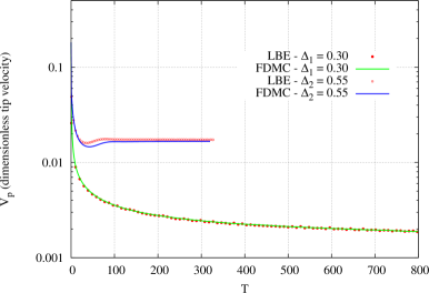
Figure 2: Dimensionless tip velocity $V_{p}$ as a function of time for FDMC (solid lines) and LBE (red dots) for two undercoolings $\Delta_{1}=0.30$ and $\Delta_{2}=0.55$ (from [49]). Parameters are $\kappa=4$, $\lambda^{\star}=6.3826$, $d_{0}=0.1385$ and $\varepsilon_{s}=0.05$.

4 Anisotropy functions

This section focuses on the $a_{s}(\mathbf{n})$ function responsible for the characteristic shapes of crystals. In LB schemes for phase-field model, the $a_{s}$ function appears (i) in the phase-field equation (Eq. (6a)), (ii) in the vectorial function $\boldsymbol{\mathcal{N}}(\mathbf{x},\,t)$ of e.d.f. (Eq. (6b)) and (iii) in the relaxation rate $\eta_{\phi}$ (Eq. (8c)). This section investigates the anisotropy function for which the growth of branches are not directed along the main axes of the coordinate system, i.e. we focus on the anisotropy function for a preferential growth other than $\left\langle 10\right\rangle$ in 2D and $\left\langle 100\right\rangle$ in 3D. First, main formulations of the $a_{s}$ function are reminded and next, effects of gradient calculation on the crystal shape are presented.

4.1 Spherical or Cartesian formulations

Two main formulations are used in the literature to simulate dendritic crystals. In 2D, the standard formulations are based on the angle $\varphi\equiv\varphi(\mathbf{x},\,t)$ (e.g. [5]) between the normal vector of the interface and the $x$-axis. In phase-field models, this angle is expressed in terms of derivatives of the phase-field $\phi$. Definition of normal vector is given by $\mathbf{n}=-\boldsymbol{\nabla}\phi/\bigl{|}\boldsymbol{\nabla}\phi\bigr{|}$ and its components are $n_{x}=-\partial_{x}\phi/\bigl{|}\boldsymbol{\nabla}\phi\bigr{|}$ and $n_{y}=-\partial_{y}\phi/\bigl{|}\boldsymbol{\nabla}\phi\bigr{|}$. The angle $\varphi$ is defined by: $\tan\varphi=\sin\varphi/\cos\varphi=n_{y}/n_{x}=\partial_{y}\phi/\partial_{x}\phi$ i.e. it can be obtained by the relationship $\varphi=\tan^{-1}(\partial_{y}\phi/\partial_{x}\phi)$. Therefore, if $\partial_{x}\phi\neq 0$, the angle $\varphi$ is calculated from the phase-field $\phi$. The standard form of $a_{s}(\varphi)$ in 2D is:

$$a_{s}(\varphi)=1+\varepsilon_{s}\cos\left[q\left(\varphi(\mathbf{x},\,t)-\varphi_{0}\right)\right],$$ (10)

where $\varphi_{0}$ is a reference angle. Both coefficients $\varepsilon_{s}>0$ and $q$ are respectively the strength and mode of anisotropy. For instance, the choice $q=4$ and $\varphi_{0}=0$ leads to the development of crystal with four tips directed along the main axes $x$ and $y$. Indeed, the growth is maximal when $\cos(4\varphi)$ is equal to one, i.e. for multiple integers of $\varphi=\pi/2$. Other similar 2D formulations exist in the literature. For instance in [20]: $a_{s}(\varphi)=1+\varepsilon_{s}\left[8/3\sin^{4}(q/2(\varphi-\varphi_{0}))-1\right]$. The power four of the sine function yields an asymmetry between the maximal and minimal values of $a_{s}$. Also note the modification of $a_{s}(\varphi)$ for simulating crystals that are faceted [62, 63]. Those shapes are not studied in this work.

A formulation of $a_{s}(\varphi)$, defined by an angle $\varphi,$ is equivalent to $a_{s}(\mathbf{n})$ defined by a normal vector $\mathbf{n}$. By expanding the particular case $a_{s}(\varphi)=1+\varepsilon_{s}\cos(4\varphi)$ in powers of $\cos\varphi$ and $\sin\varphi$ (with $\cos(4\varphi)=\cos 2(2\varphi)$), and next by identifying $n_{x}=\cos\varphi$ and $n_{y}=\sin\varphi$, the 2D relationship $a_{s}(\mathbf{n})=1-3\varepsilon_{s}+4\varepsilon_{s}(n_{x}^{4}+n_{y}^{4})$ is obtained [12]. More generally, the function $\cos(q\varphi)$ can be derived from a formalism involving spherical harmonics. On a spherical surface, any scalar function can be decomposed on a basis of spherical functions depending on two angles $\varphi$ and $\theta$: the spherical harmonics. The distance $r$ is the third coordinate to define the position on a sphere. For instance $\cos(4\varphi)$ corresponds to the real part of the spherical harmonic $Y_{4,4}(\theta,\,\varphi)$ in the $XY$-plane (i.e. with $\theta=\pi/2$): $\mbox{Re}[Y_{4,4}(\pi/2,\,\varphi)]\propto\cos(4\varphi)$. The symbol $\propto$ means that the spherical harmonic $Y_{4,4}$ is proportional to that function with a normalization factor.

An application of such a formalism is given here. The $a_{s}(\mathbf{n})$ function that is derived will be used in Section 5, for comparisons between a 2D code which uses a $\varphi$-formulation and a 3D code which uses a $\mathbf{n}$-formulation. That benchmark will be carried out in order to validate numerical implementation of the directional derivatives method. If we want to derive a $a_{s}(\mathbf{n})$ function that is equivalent to $a_{s}(\varphi)=1+\varepsilon_{s}\cos(6\varphi)$, the real part of $Y_{6,6}(\theta,\,\varphi)$ is considered: $\mbox{Re(}Y_{6,6}(\theta,\,\varphi))\propto\cos(6\varphi)\sin^{6}\theta$. After developing $\cos(6\varphi)$ and using the variable change from spherical to Cartesian coordinates, $\sin\theta\cos\varphi=x/r$, $\sin\theta\sin\varphi=y/r$ and $\cos\theta=z/r$, the calculation leads to $\mbox{Re}(Y_{6,6}(\mathbf{x}))\propto(x^{6}-15x^{4}y^{2}+15x^{2}y^{4}-y^{6})/r^{6}$. After identifying $n_{x}=x/r$, $n_{y}=y/r$ and $n_{z}=z/r$, the anisotropy function is:

$$a_{s}(\mathbf{n})=1+\varepsilon_{s}(n_{x}^{6}-15n_{x}^{4}n_{y}^{2}+15n_{x}^{2}n_{y}^{4}-n_{y}^{6}).$$ (11)

Eq. (11) favors crystal growth in six main growing directions in the $XY$-plane. That function will be used in Section 5.1. The same procedure can be followed for other characteristic shapes after identification of spherical harmonics suited to the problem.

In 3D, any anisotropy function $a_{s}(\mathbf{n})$ can be expressed as a linear combination of cubic harmonics. The cubic harmonics are linear combinations of real spherical harmonics with an appropriate cubic symmetry [64, 65, 66]. For instance, function $Q(\mathbf{n})=n_{x}^{4}+n_{y}^{4}+n_{z}^{4}$ of Eq. (1d), which favors the growth in $\left\langle 100\right\rangle$ preferential direction, can be derived from the cubic harmonic $K_{4,1}(\theta,\,\varphi)\propto\left[5\cos^{4}\theta-3+5\sin^{4}\theta(\cos^{4}\varphi+\sin^{4}\varphi)\right]$. After the variable change in Cartesian coordinates, that function becomes $K_{4,1}(\theta,\,\varphi)\propto\left[5(n_{x}^{4}+n_{y}^{4}+n_{z}^{4})-3\right]$. By considering an additional cubic harmonic $K_{6,1}$, the $a_{s}(\mathbf{n})$ function can be generalized for other growing directions. For instance, the $\left\langle 110\right\rangle$-direction can be simulated by [67]:

$$a_{s}(\mathbf{n}) =1+\varepsilon_{s}\left(\sum_{\alpha=x,y,z}n_{\alpha}^{4}-\frac{3}{5}\right)+\gamma\left(3\sum_{\alpha=x,y,z}n_{\alpha}^{4}+66n_{x}^{2}n_{y}^{2}n_{z}^{2}-\frac{17}{7}\right),$$ (12)

where $\varepsilon_{s}$ is the anisotropy strength in the $\left\langle 100\right\rangle$-directions and $\gamma$ is the anisotropy strength in the $\left\langle 110\right\rangle$-directions. The first term of the right-hand side is the cubic harmonic $K_{0,0}=1$, the second one is $K_{4,1}\propto[5Q(\mathbf{n})-3]$ and the last one is the cubic harmonic $K_{6,1}\propto[462S(\mathbf{n})+21Q(\mathbf{n})-17]$ with $S(\mathbf{n})=n_{x}^{2}n_{y}^{2}n_{z}^{2}$. We can refer to [64, 68] for other cubic harmonics of higher order, defined in terms of functions $Q(\mathbf{n})$ and $S(\mathbf{n})$.

Let us mention that several experiments and simulations, involving the anisotropy function (Eq. (12)), were carried out in the literature to study the <<dendrite orientation transition>> from $\left\langle 100\right\rangle$ to $\left\langle 110\right\rangle$ [69, 70]. In those references, phase-field simulations are performed by varying systematically the anisotropy parameters $\varepsilon_{s}$ and $\gamma$ to explore the role of these parameters on the resulting microstructures. Simulations are carried out for pure substance and binary mixture for equiaxed crystals and directional solidification.

In order to see the influence of each term of Eq. (12), a graphical representation is plotted on a spherical surface. First, the phase-field $\phi(\mathbf{x},\,0)$ is initialized (by using Eq. (3)) inside a cubic domain composed of $200^{3}$ nodes. The initial sphere is set at the center of the domain $\mathbf{x}_{s}=(100,\,100,\,100)^{T}$ with a radius equals to $R_{s}=50$ lattice units (l.u.). Next, the components $n_{x}$, $n_{y}$ and $n_{z}$ are derived by calculating the gradient of $\phi$. Finally, each term of Eq. (12) is calculated and post-processed on a spherical surface of radius $R_{s}$ and centered at $\mathbf{x}_{s}$. Results are presented in Figs. 3 for various values of $\varepsilon_{s}$ and $\gamma$. On those figures, the red and blue areas correspond to the zones for which the growth is respectively maximal and minimal. All figures are plotted for a same orientation of the coordinate system to facilitate the comparison between functions. As expected, function $Q(\mathbf{n})$ favors growth in the $\left\langle 100\right\rangle$-direction (Fig. 3a); $S(\mathbf{n})$ favors growth in the $\left\langle 111\right\rangle$-direction (Fig. 3b), and $a_{s}(\mathbf{n})$ defined by Eq. (12) with $\varepsilon_{s}=0$ and $\gamma=-0.02$ favors growth in the $\left\langle 110\right\rangle$-direction (Fig. 3e). Simulations of crystal growth with those three anisotropy functions will be carried out in Section 5.

(a) $Q(\mathbf{n})=n_{x}^{4}+n_{y}^{4}+n_{z}^{4}$		(b) $S(\mathbf{n})=n_{x}^{2}n_{y}^{2}n_{z}^{2}$		(c) $3Q(\mathbf{n})+66S(\mathbf{n})$
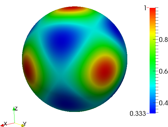
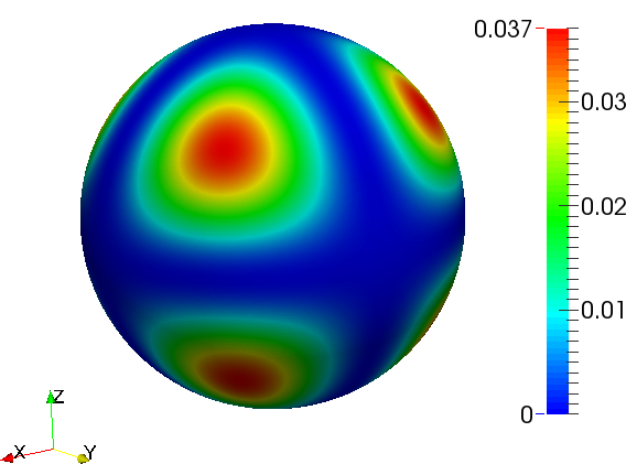
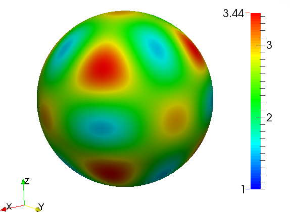
(d) $a_{s}(\mathbf{n})$ with $\varepsilon_{s}=0.02$, $\gamma=-0.02$		(e) $a_{s}(\mathbf{n})$ with $\varepsilon_{s}=0$, $\gamma=-0.02$		(f) $a_{s}(\mathbf{n})$ with $\varepsilon_{s}=0.05$, $\gamma=0.02$

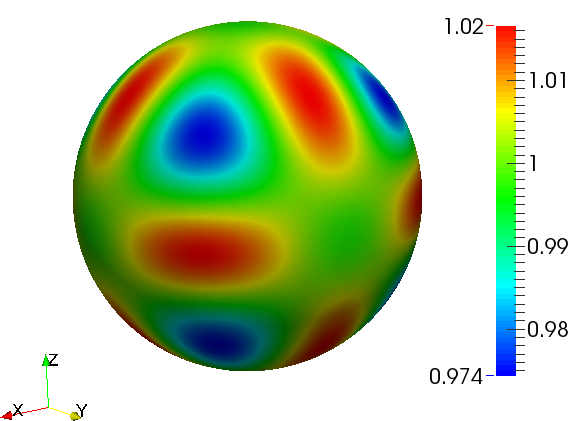
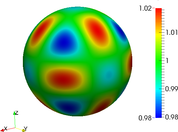
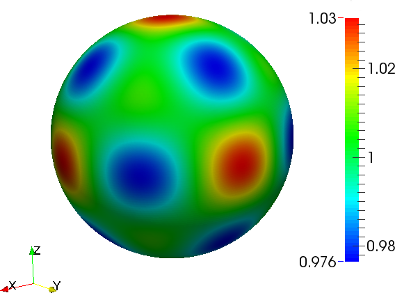
Figure 3: Graphical representation of each term of Eq. (12).

4.2 Effect of directional derivatives of gradients in LB schemes

For each formulation of $a_{s}$, it is necessary to compute the gradient of $\phi$ for deriving the components of $\mathbf{n}$. It is also necessary to compute the derivatives of $a_{s}(\mathbf{n})$ with respect to $\partial_{x}\phi$, $\partial_{y}\phi$ and $\partial_{z}\phi$ involved in the vector $\boldsymbol{\mathcal{N}}(\mathbf{x},\,t)$. Two approaches were compared in this work. In the first one, the gradient is calculated by using the classical formula of central finite differences, i.e. in 2D: $\partial_{x}\phi\simeq(\phi_{j+1,\,k}-\phi_{j-1,\,k})/2\delta x$ and $\partial_{y}\phi\simeq(\phi_{j,\,k+1}-\phi_{j,\,k-1})/2\delta x$, where $j$ and $k$ are indexes of coordinates $x$ and $y$.

In the second approach, the method based on the directional derivatives is applied. The method has already demonstrated its performance for hydrodynamics problem in order to reduce parasitic currents for two-phase flow problem [51, 52, 50]. The directional derivative is the derivative along each moving direction on the lattice. Taylor’s expansion at second-order of a differentiable scalar function $\phi(\mathbf{x})$ at $\mathbf{x}+\mathbf{e}_{i}\delta x$ and $\mathbf{x}-\mathbf{e}_{i}\delta x$ yields the following approximation of directional derivatives:

$$\mathbf{e}_{i}\cdot\boldsymbol{\nabla}\phi\bigr{|}_{\mathbf{x}}=\frac{1}{2\delta x}\left[\phi(\mathbf{x}+\mathbf{e}_{i}\delta x)-\phi(\mathbf{x}-\mathbf{e}_{i}\delta x)\right].$$ (13a)

The number of directional derivatives is equal to the number of moving direction $\mathbf{e}_{i}$ on the lattice i.e. $N_{pop}$. The gradient is obtained by:

$$\boldsymbol{\nabla}\phi\bigr{|}_{\mathbf{x}}=\frac{1}{e^{2}}\sum_{i=0}^{N_{pop}}w_{i}\mathbf{e}_{i}\left(\mathbf{e}_{i}\cdot\boldsymbol{\nabla}\phi\bigr{|}_{\mathbf{x}}\right).$$ (13b)

The three components of gradient $\partial_{x}\phi$, $\partial_{y}\phi$ and $\partial_{z}\phi$ are obtained by calculating each directional derivative with the relationship (13a) and next, by calculating the moment of first order with Eq. (13b). In Eq. (13b), each direction is weighted by coefficients $w_{i}$ and the sum is normalized by factor $1/e^{2}$. For gradient computation, the number and directions of directional derivatives are consistent with the number and moving directions of distribution functions. The directional derivatives method is consistent with the lattice that are used for simulations. This is the main advantage of the method. Indeed, on lattices D2Q9 and D3Q15, the distribution functions $f_{i}$ and $g_{i}$ can move in diagonal directions. With this method, each derivative along the direction of propagation is used to calculate the gradient. Thus, the derivatives contain the contributions of diagonal directions of lattices D2Q9 and D3Q15. Those relationships can also be used for other lattices, such as D3Q19 and D3Q27. Note that the second-order central difference is used in Eq. (13a) for approximating the directional derivatives. Other approximations exist [50] such as the first-order and second-order upwind schemes (or biased differences) respectively defined by $\mathbf{e}_{i}\cdot\boldsymbol{\nabla}^{up_{1}}\phi\bigr{|}_{\mathbf{x}}=[\phi(\mathbf{x}+\mathbf{e}_{i}\delta x)-\phi(\mathbf{x})]$/$\delta x$ and $\mathbf{e}_{i}\cdot\boldsymbol{\nabla}^{up_{2}}\phi\bigr{|}_{\mathbf{x}}=\left[-\phi(\mathbf{x}+2\mathbf{e}_{i}\delta x)+4\phi(\mathbf{x}+\mathbf{e}_{i}\delta x)-3\phi(\mathbf{x})\right]/(2\delta x)$. If necessary, the second derivative of $\phi$ can also be obtained by $(\mathbf{e}_{i}\cdot\boldsymbol{\nabla})^{2}\phi\bigr{|}_{\mathbf{x}}=\left[\phi(\mathbf{x}+\mathbf{e}_{i}\delta x)-2\phi(\mathbf{x})+\phi(\mathbf{x}-\mathbf{e}_{i}\delta x)\right]/\delta x^{2}$. Here, the central difference approximation Eq. (13a) is applied for all simulations.

We compare the impact of both methods on the solution $\phi$. We simulate Eqs. (1a)–(1c) in 2D with $a_{s}(\varphi)$ defined by Eq. (10) for $q=6$ and $\varphi_{0}=0$. Components of gradient are calculated by using first (i) the classical formula of central finite difference ($FD$) and second (ii) the directional derivatives ($DD$) given by Eqs. (13a)–(13b). For simulations, the mesh is composed of 800$\times$800 nodes. The parameters are $\delta x=\delta y=0.01$, $\delta t=1.5\times 10^{-5}$, $\tau_{0}=1.5625\times 10^{-4}$, $W_{0}=0.0125$, $\kappa=1$, the undercooling is $\Delta=0.30$, $\lambda=10$, $\varepsilon_{s}=0.05$. The seed is initialized at the center of the domain $\mathbf{x}_{c}=(400,\,400)$, and the radius is $R_{s}=10$ lattice unit (l.u.).

For both methods, we present on Fig. 4 the solution $\phi=0$ at $t=10^{5}\delta t$ (red curve) and the same solution with a rotation of 60° (blue curve). When the gradients are calculated with a finite differences method, the phase-field $\phi=0$ does not match perfectly with its rotation of 60° (Fig. 4a). The phase-field is not any more isotropic and the numerical solution presents some lattice anisotropy effects. Those effects can be seen more precisely on Fig. 5a which plots the difference $\phi^{rot}(\mathbf{x})-\phi(\mathbf{x})$ with the $FD$ method. In two main directions defined by $\mathbf{n}_{a}=(1,\,0)$ and $\mathbf{n}_{b}=(1/2,\,-\sqrt{3}/2)$ the differences are maximal at the tips (respectively $1.446$ and $-1.454$), whereas in the third direction $\mathbf{n}_{c}=(1/2,\,+\sqrt{3}/2)$ the difference is lower than $0.01$. When the gradients are calculated with the $DD$ method, the phase-field $\phi=0$ is much more isotropic (Fig. 4b) as confirmed by the differences $\phi^{rot}(\mathbf{x})-\phi(\mathbf{x})$ plotted on Fig.5b. The differences are now more uniformly distributed inside the domain and the maximal and minimal values are divided by a factor $14$ (respectively $0.1$ and $-0.103$). The lattice anisotropy is reduced.

In order to quantify the errors, the $\ell^{2}$ relative error norm is calculated with two $\phi$-profiles plotted along two directions $\mathbf{n}_{a}$ and $\mathbf{n}_{b}$ defined above. The $\ell^{2}$ relative error norm is defined by:

$$\mbox{Err}_{\ell^{2}}=\sqrt{\frac{\sum_{j}^{N_{j}}(\phi_{a,j}-\phi_{b,j})^{2}}{\sum_{j}^{N_{j}}\phi_{a,j}^{2}}},$$ (14)

where $\phi_{a}$ and $\phi_{b}$ are the phase-fields collected along the directions $\mathbf{n}_{a}$ and $\mathbf{n}_{b}$ respectively. The profiles of $\phi_{a}$ and $\phi_{b}$ are presented on Figs. 6a,b for both methods of gradient computation. The phase-field $\phi_{a}$ sampled along the direction $\mathbf{n}_{a}$ is taken as a reference for the error calculation. $N_{j}$ is the total number of values and $j$ is the index. The $\ell^{2}$ relative error for the finite difference method is $\mbox{Err}{}_{\ell^{2}}^{FD}=1.71\times 10^{-1}$ and the relative error for the directional derivatives method is $\mbox{Err}{}_{\ell^{2}}^{DD}=3.04\times 10^{-3}$. The error is decreased by a factor $56$ by using the $DD$ method. This problem of lattice anisotropy is decreased when the relationships (13a) and (13b) are applied to calculate the gradients (Fig. 4b and Fig. 6b).

(a) $\phi=0$ with standard finite differences		(b) $\phi=0$ with directional derivatives method

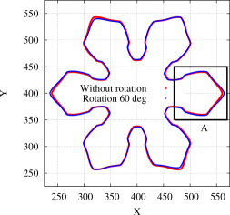
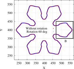
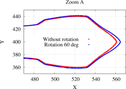
Figure 4: Effect of using a central finite difference method (a), or a directional derivatives method (b) to calculate the gradients of $\phi$ on a D2Q9 lattice. Without directional derivatives, the phase-field $\phi=0$ (red) at $t=10^{5}\delta t$ does not match with its rotation of 60° (blue). The rotation matches perfectly when the directional derivatives method is applied.

(a) Difference $\phi^{rot}(\mathbf{x})-\phi(\mathbf{x})$ with $FD$		(b) Difference $\phi^{rot}(\mathbf{x})-\phi(\mathbf{x})$ with $DD$

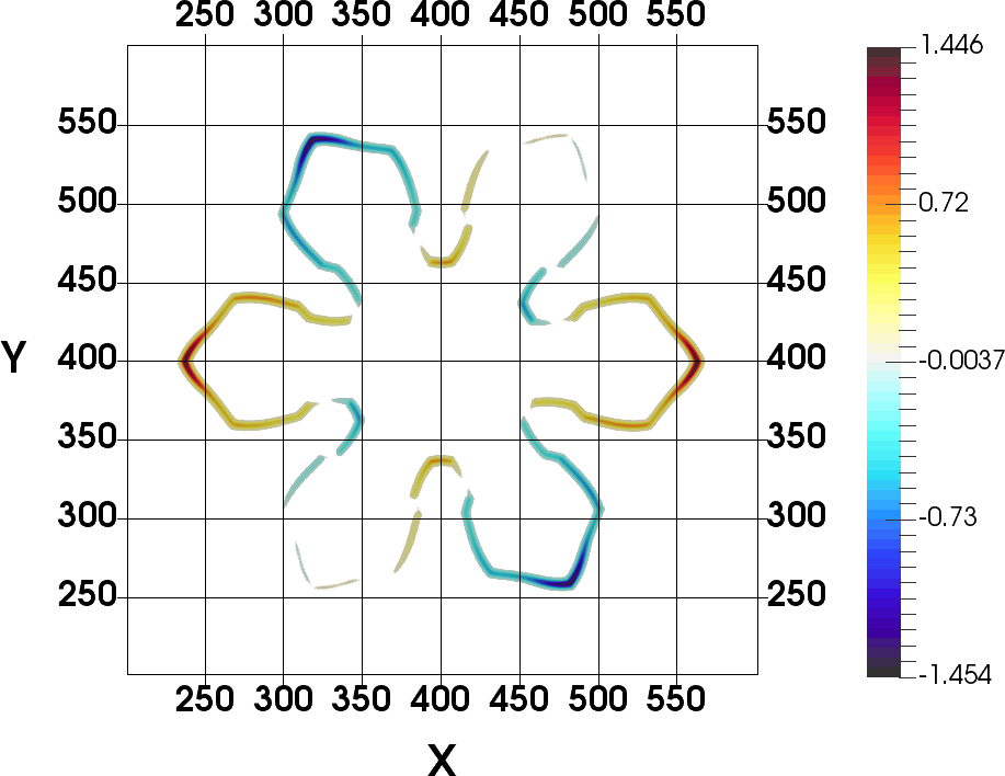
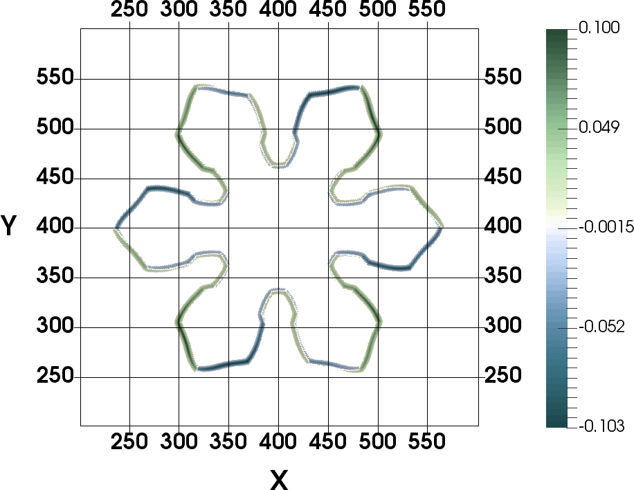
Figure 5: Differences between $\phi^{rot}(\mathbf{x})-\phi(\mathbf{x})$ (a) with Finite Difference and (b) with Directional Derivatives. $\phi^{rot}(\mathbf{x})$ is obtained from $\phi(\mathbf{x})$ after a rotation of 60°.

(a) Profiles with finite differences		(b) Profiles with directional derivatives

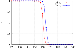
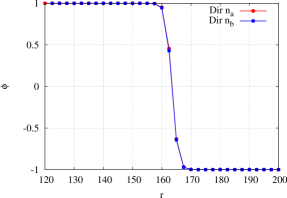
Figure 6: $\phi$-profiles along the directions $\mathbf{n}_{a}=(1,\,0)$ and $\mathbf{n}_{b}=(1/2,\,-\sqrt{3}/2)$. (a) With a finite difference method the relative error ($\ell^{2}$-norm) is $1.71\times 10^{-1}$ and (b) its value is equal to $3.07\times 10^{-3}$ with a directional derivatives method.

The origin of those differences can be understood when the $a_{s}$ function is plotted as a function of position (Fig. 7). At $t=10^{5}\delta t$, with the finite differences method, the values of $a_{s}$ depend on the direction of growth, the function is not isotropic by rotation. In other words, on Fig. 7a, the first pattern inside the box B, which corresponds to a direction of growth $\mathbf{n}_{a}$, is different of the second one inside the box A corresponding to a direction $\mathbf{n}_{c}$. The pattern of $a_{s}$ is not periodic. On the contrary, with the directional derivatives method, the patterns in boxes A and B are identical (Fig. 7b). By considering the diagonals of the lattice in the calculation of gradient, $a_{s}$ is more accurate and fully symmetric by rotation. Let us mention that those differences do not appear when $q=4$, even for gradients computed by central finite difference, because the growth occurs in the main direction of the coordinate system: $x$- and $y$-axis.

(a) $a_{s}(\varphi)$ with finite differences method		(b) $a_{s}(\varphi)$ with directional derivatives method

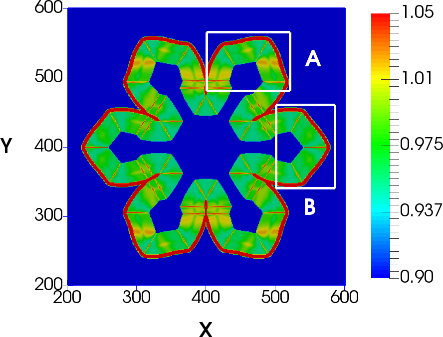
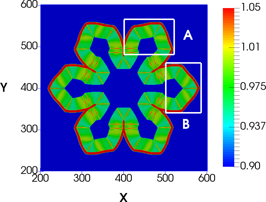
Figure 7: Anisotropy function $a_{s}(\varphi)$ at $t=10^{5}\delta t$. (a) With a finite differences method the values of the $a_{s}$ function are different inside boxes A and B, whereas (b) with a directional derivatives method, they are identical.

Finally, the whole approach (LB+DD) is applied to simulate again the crystal growth with $q=6$ and $\varphi_{0}=0$, by modifying the undercooling and the interfacial kinetic. In this simulation, we choose the parameter $\lambda$ such as the interfacial kinetic (Eq. (2b)) is canceled. The condition $\beta=0$ is satisfied for one particular value of $\lambda$: $\lambda^{\star}=\kappa\tau_{0}/a_{2}W_{0}^{2}$. By considering $W_{0}=1$ and $\tau_{0}=1$, the coefficient $\lambda^{\star}$ is equal to $\lambda^{\star}=\kappa/a_{2}=1.59566\kappa$. For a thermal diffusivity equals to $\kappa=4$, we obtain $\lambda^{\star}=6.3826$ and the capillary length is $d_{0}=0.1385$. The mesh is composed of 800$\times$800 nodes. Parameters are $\delta x=\delta y=0.4$, $\delta t=0.008$, the undercooling is $\Delta=0.55$ and the anisotropic strength is $\varepsilon_{s}=0.05$. The radius of the initial seed is $R_{s}=10$ lattice unit (l.u.). Results are presented on Fig. 8 at $t=4\times 10^{4}\delta t$. The anisotropy function is plotted on Fig. 8a. On that figure, we can observe that the pattern is identical in each branch of the crystal. The $a_{s}$ function is symmetric by rotation of 60°. On Fig. 8b, the temperature field is plotted and the evolution of $\phi$ is superimposed at four different times (black lines). We can check that the solution of $\phi$ is isotropic, the phase-field matches perfectly with its rotation of 60°.

(a) Anisotropy function $a_{s}(\varphi)$		(b) Temperature field $u$ and evolution of $\phi=0$

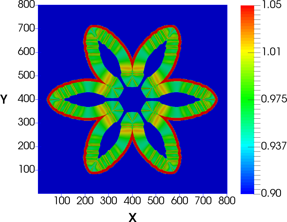
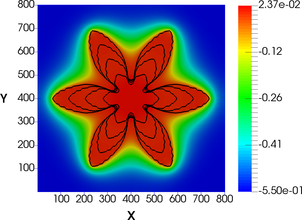
Figure 8: Simulation for $\Delta=0.55$ and $q=6$, results at $t=4\times 10^{4}\delta t$. (a) Anisotropy function $a_{s}(\varphi)$ with directional derivatives. (b) Dimensionless temperature $u$ and phase-field $\phi=0$ (black lines) at $t=1,\,2,\,3,\,4\times 10^{4}\delta t$.

4.3 Simultaneous growth of crystals with different anisotropy functions

Now, we are interested in the simultaneous growth of several crystals with different numbers of branches and different angle of reference $\varphi_{0}$. The difficulty does not lie in the growth of several crystals since their number is naturally taken into account in the phase-field model, more precisely in the initial condition of $\phi$. For instance, for simulating the growth of three crystals, three initial grains are set with the relationship (3). Each of them will grow progressively during the simulation but they will have the same anisotropy function. Here, we consider that each crystal can be defined by its own anisotropy function $a_{s}(\mathbf{n})$.

For that purpose, we consider that this function depends on a new index $I\equiv I(\mathbf{x},\,t)$:

$$a_{s}^{(I)}(\mathbf{x},\,t)=1+\varepsilon_{s}^{(I)}\cos\left[q^{(I)}\left(\varphi(\mathbf{x},\,t)-\varphi_{0}^{(I)}\right)\right],$$ (15)

where $I$ is a field indicating the crystal number. This new function depends on position and time and varies from $1$ to $N_{I}$ where $N_{I}$ is the number of crystals: it is equal to 1 for the first crystal; 2 for the second one; 3 for the third one, and so on … Its value is zero everywhere else. For example in 2D, if we choose $N_{I}=3$ crystals, with $q^{(1)}=4$, $q^{(2)}=5$ and $q^{(3)}=6$ respectively, the evolution of $I(\mathbf{x},\,t)$ has to be updated at each time step. After initialization of $\phi(\mathbf{x},\,t)$ and $I(\mathbf{x},\,t)$, the nodes surrounding each crystal are selected with a criterion based on the variation of $\phi$: $\bigl{|}\boldsymbol{\nabla}\phi\bigr{|}>\xi$ where $\xi$ is a small numerical value. This criterion is used to identify all nodes that have a zero value and located near the diffuse zone of each crystal. Then the index of those nodes takes the value of the nearest node having an index different to zero.

Three seeds are initialized in a computational domain composed of 1200$\times$1200 nodes. The radius is set at $R_{s}=8$ l.u for each of them and positions are $\mathbf{x}^{(1)}=(350,\,350)$, $\mathbf{x}^{(2)}=(850,\,400)$ and $\mathbf{x}^{(3)}=(600,\,820)$. An angle $\varphi_{0}^{(1)}=45$° is set for the first crystal and $\varphi_{0}^{(2)}=5$° for the second one. Parameters are $\delta x=5\times 10^{-3}$, $\delta t=5\times 10^{-6}$, $W_{0}=0.012$, $\tau_{0}=10^{-4}$, $\lambda=10$, $\varepsilon_{s}^{1,\,2,\,3}=0.04$, $\kappa=0.7$ and $\Delta=0.3$. The small numerical value for the criterion is $\xi=10^{-7}$. Results are presented on Fig. 9a. Black lines represent the time evolution of $\phi=0$, and the temperature field is plotted at the end of simulation. Crystals have respectively four, five and six tips. On the figure, for short times ($<10^{5}\delta t$), the branch size is identical for each crystal. At $t=10^{5}\delta t$ the pattern of each branch for each crystal is identical as confirmed by Fig. 9b. On the other hand, for greater times, some branches are smaller because of the influence of other crystals. The growth of those branches is limited by the temperature field that is uniform and higher in the interaction zone of crystals. In this area, the latent heat released during the solidification is evacuated less rapidly in the system and the speed of growth decreases.

(a) Temperature field $u$ and evolution of $\phi=0$	(b) Anisotropy function $a_{s}^{(I)}(\mathbf{x},\,t)$ at $t=10^{5}\delta t$

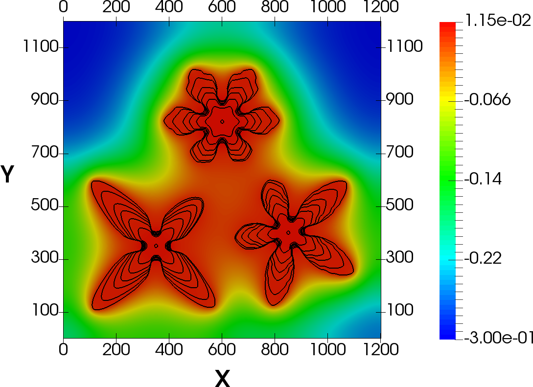
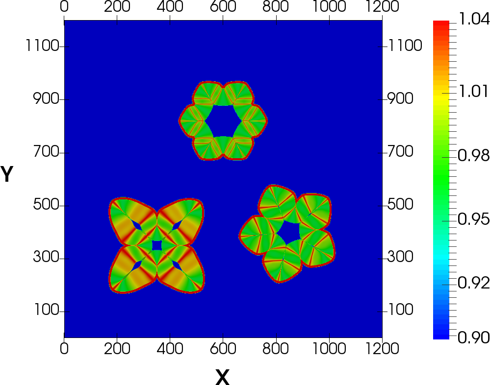
Figure 9: Simultaneous growth of three crystals with 4, 5 and 6 tips. (a) phase-field $\phi=0$ at $t=0,\,2.5,\,5,\,7.5,\,10,\,15,\,20\times 10^{4}\delta t$ with temperature field at $t=20\times 10^{4}\delta t$. (b) Anisotropy function $a_{s}^{(I)}(\mathbf{x},\,t)$ at $t=10^{5}\delta t$.

5 3D simulations

In this section, we present 3D simulations based on anisotropy functions defined in section 4. Let us remind that several experiments and simulations were carried out in the literature to study the <<dendrite orientation transition>> from $\left\langle 100\right\rangle$ to $\left\langle 110\right\rangle$ for a pure substance and binary mixtures [69, 70]. Here, those simulations are performed to demonstrate the flexibility of the LB method and its ability to simulate various crystal shapes. Once the anisotropy function $a_{s}(\mathbf{n})$ is modified and its derivatives with respect to $\partial_{\alpha}\phi$ ($\alpha=x,\,y,\,z$) calculated, implementation of 3D schemes is straightforward by modifying the lattices. In subsection 5.1, the directional derivatives method implemented in the 3D code is checked with the 2D code validated in [49] with a finite difference code. In subsection 5.2, 3D simulations with three different anisotropy functions will be presented.

5.1 Comparisons between 2D and 3D codes

In order to check numerical implementation of directional derivatives method in the 3D code, a comparison is carried out with the 2D one. The validation is based on a comparison of Eq. (11), established in subsection 4.1, that is equivalent to the 2D function $a_{s}(\varphi)=1+\varepsilon_{s}\cos(6\varphi)$. Simulations of crystal growth are performed with a mesh composed of $301{}^{2}$ nodes in 2D and $301\times 301\times 4$ nodes in 3D. Only four nodes are used for the third dimension $z$ because Eq. (11) favors the growth of six tips in the $XY$-plane.

For both codes the parameters are set as follows. The space step is equal to $\delta x=0.01$ and the time step is chosen such as $\delta t=1.5\times 10^{-5}$. The initial condition is a diffuse sphere initialized at the domain center with a radius equals to $R_{s}=6$ lattice unit (l.u.). All boundary conditions are zero-flux types. The initial undercooling is uniform and equal to $u=-0.3$ and the thermal diffusivity is equal to $\kappa=0.7$. Parameters of the phase-field are $W_{0}=0.0125$, $\tau_{0}=1.5625\times 10^{-4}$, $\lambda=10$ and $\varepsilon_{s}=0.05$.

Results are presented on Fig. 10. On this figure, the left plot presents the phase-field $\phi=0$ for $a_{s}(\varphi)$ in 2D (blue squares) and $a_{s}(\mathbf{n})$ in 3D (red dots) at four times $t=2,\,4,\,6,\,8\times 10^{3}\delta t$. The shape with six tips in the $XY$-plane is well reproduced by using the anisotropy function defined by Eq. (11) in the 3D code. For both codes, several iso-values of temperature field at $t=8\times 10^{3}\delta t$ are superimposed on the right plot. The 3D implementation of the LB schemes is validated.

(a) Phase-field $\phi=0$ ($t=t^{\prime}\times 10^{3}\delta t$)		(b) Temperature iso-values

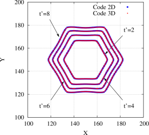
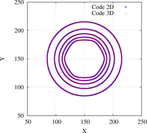
Figure 10: (a) Iso-values $\phi=0$ for Eq. (10) with $q=6$ and $\varphi_{0}=0$ (blue squares; 2D code) and Eq. (11) (red dots; 3D code) at $t=3\times 10^{3}\delta t$ and $t=8\times 10^{3}\delta t$. (b) Iso-values $u=-0.25$, $-0.2$, $-0.15$, $-0.1$ and $-0.05$ at $t=8\times 10^{3}\delta t$ in 2D (blue square) and 3D (red dots).

5.2 Simulations with non standard anisotropy functions

In this section, 3D simulations are carried out by using three anisotropy functions $a_{s}(\mathbf{n})$. The first anisotropy function is the standard one, defined by Eq. (1d) with $\varepsilon_{s}=0.05$. That function favors the growth in the $\left\langle 100\right\rangle$-direction (see Fig. 3a). The second one is defined by Eq. (12) which favors the crystal development in the $\left\langle 110\right\rangle$-direction if $\varepsilon_{s}=0$ and $\gamma=-0.02$ (see Fig. 3e). The last one is defined by:

$$a_{s}(\mathbf{n})=66\gamma n_{x}^{2}n_{y}^{2}n_{z}^{2},$$ (16)

with $\gamma=0.02$. That function favors the growth in the $\left\langle 111\right\rangle$-direction (see Fig. 3b).

For each simulation, the computational domain is composed of $351^{3}$ nodes and the undercooling is fixed at $\Delta=0.30$. The space step is $\delta x=0.01$ and the time step is $\delta t=1.5\times 10^{-5}$. The seed is initialized at the center $\mathbf{x}_{c}=(175,\,175,\,175)^{T}$ of the domain. The interface thickness is equal to $W_{0}=0.0125$, the kinetic time is $\tau_{0}=1.5625\times 10^{-4}$, the coupling coefficient is $\lambda=10$, and the thermal diffusivity is $\kappa=1$.

Dendritic shapes $\phi=0$ of each crystal are presented on Fig. 11 for a same orientation of the coordinate system. Directions of growth $\left\langle 100\right\rangle$, $\left\langle 110\right\rangle$ and $\left\langle 111\right\rangle$ are presented respectively on Figs. 11a (dendrite A), 11b (dendrite B) and 11c (dendrite C). For dendrite B, as expected in view of Fig. 3e, the crystal shape presents twelve tips: four contained in the $XY$-plane centered at $\mathbf{x}_{c}$, four other above this plane and four below. Finally, for dendrite C, we can see four tips above the same plane and four below, as expected in view of Fig. 3b.

In order to check the isotropy of phase-field $\phi=0$, obtained with the directional derivatives method, several slices are carried out for each dendrite. The center of each plane is $\mathbf{x}_{c}$. For dendrite A, two slices are carried out in the planes of normal vectors $\mathbf{n}_{1}^{A}=(1,\,0,\,0)$ and $\mathbf{n}_{2}^{A}=(0,\,1,\,0)$. Solution $\phi=0$ of the $\mathbf{n}_{1}^{A}$-plane ($YZ$-plane) is compared to the second one ($\mathbf{n}_{2}^{A}$-plane) after a rotation of 90° around the $z$-axis for the second plane (see Fig. 12a). For dendrite B, two slices of normal vectors $\mathbf{n}_{1}^{B}=(1,\,1,\,1)$ and $\mathbf{n}_{2}^{B}=(1,\,1,\,-1)$ are carried out. The solution $\phi=0$ from the first plane is compared with the second one obtained after rotation (see Fig. 12b). Finally, for dendrite C, the phase-fields $\phi=0$ from planes of normal vectors $\mathbf{n}_{1}^{C}=(1,\,1,\,0)$ and $\mathbf{n}_{2}^{C}=(1,\,-1,\,0)$ are compared on Fig. 12c after a rotation of -45° for the first plane and +45° for the second one. The rotation is performed around the $z$-axis. For each dendrite, the phase-fields are superimposed and the directional derivatives method gives satisfying results for the numerical isotropy of the solution.

(a) Dendrite A: growing direction $\left\langle 100\right\rangle$	(b) Dendrite B: growing direction $\left\langle 110\right\rangle$	(c) Dendrite C: growing direction $\left\langle 111\right\rangle$

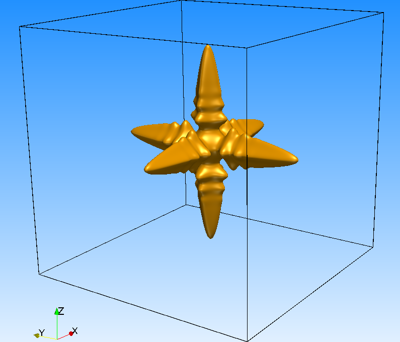
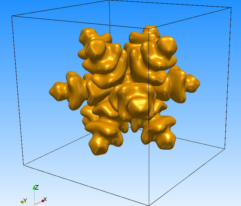
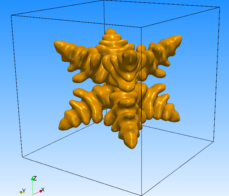
Figure 11: Dendritic shapes $\phi=0$ for $a_{s}(\mathbf{n})$ defined by (a) Eq. (1d) with $\varepsilon_{s}=0.05$ at $t=5\times 10^{3}\delta t$; (b) Eq. (12) with $\varepsilon_{s}=0$ and $\gamma=-0.02$ at $t=2.5\times 10^{4}\delta t$; (c) Eq. (16) with $\gamma=0.02$ at $t=1.5\times 10^{4}\delta t$.

(a) Slices for dendrite A; planes (c) Slices for dendrite C; planes of normal vectors $\mathbf{n}_{1}^{A}$ and $\mathbf{n}_{2}^{A}$ of normal vectors $\mathbf{n}_{1}^{C}$ and $\mathbf{n}_{2}^{C}$

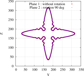
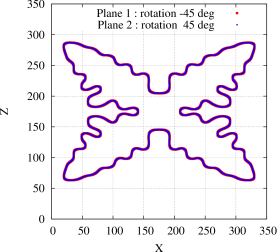
(b) Slices for dendrite B; planes of normal vectors $\mathbf{n}_{1}^{B}$ and $\mathbf{n}_{2}^{B}$

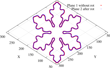
Figure 12: All planes are centered at $\mathbf{x}_{c}=(175,\,175,\,175)^{T}$. (a) Growth in $\left\langle 100\right\rangle$-direction: planes of normal vectors $\mathbf{n}_{1}^{A}=(1,\,0,\,0)$ and $\mathbf{n}_{2}^{A}=(0,\,1,\,0)$. Phase-field $\phi=0$ from the first plane (red) matches perfectly $\phi=0$ from the second plane (blue) after rotation of 90° around the $z$-axis. (b) Growth in $\left\langle 110\right\rangle$-direction: planes of normal vector $\mathbf{n}_{1}^{B}=(1,\,1,\,1)$ and $\mathbf{n}_{2}^{B}=(1,\,1,\,-1)$. Phase-field $\phi=0$ from the first plane (red) matches perfectly $\phi=0$ from the second plane (blue) after rotation. (c) Growth in $\left\langle 111\right\rangle$-direction: planes of normal vectors $\mathbf{n}_{1}^{C}=(1,\,1,\,0)$ and $\mathbf{n}_{2}^{C}=(1,\,-1,\,0)$. Phase-field from the first plane rotated from -45° around the $z$-axis (red) matches perfectly $\phi=0$ from the second plane rotated from 45° (blue).

On Fig. 11c, which corresponds to the dendrite C, we can observe a threefold symmetry for the secondary branches that appear along the main directions of growth $\left\langle 111\right\rangle$. The threefold symmetry explains why, in the slices of Fig. 12c, the secondary branches appear only on one side of each branch. The branches are not symmetric in those planes. For dendrites A and B, the symmetry is fourfold and the branches are fully symmetric on Figs. 12a and 12b. For dendrite C, the origin of the threefold symmetry can be understood by analyzing the $a_{s}(\mathbf{n})$ function and its derivatives with respect to each component $\partial_{x}\phi$, $\partial_{y}\phi$ and $\partial_{z}\phi$, i.e. the vector $\boldsymbol{\mathcal{N}}^{\prime}(\mathbf{x},\,t)$:

$$\boldsymbol{\mathcal{N}}^{\prime}(\mathbf{x},\,t)=\left(\frac{\partial a_{s}(\mathbf{n})}{\partial(\partial_{x}\phi)},\,\frac{\partial a_{s}(\mathbf{n})}{\partial(\partial_{y}\phi)},\,\frac{\partial a_{s}(\mathbf{n})}{\partial(\partial_{z}\phi)}\right)^{T}.$$ (17)

For an anisotropy function defined by Eq. (16), the $a_{s}(\mathbf{n})$ function and the streamlines of vectors $\boldsymbol{\mathcal{N}}^{\prime}(\mathbf{x})$ are plotted on a spherical surface (Fig. 13a). Here, the <<streamlines>> are the curves that are tangent to vectors $\boldsymbol{\mathcal{N}}^{\prime}(\mathbf{x})$. The same word is used by analogy to streamlines that are tangent to the velocity fields in fluid flow problems. On figure 13a, the anisotropy function is the colored field and the streamlines are the white lines. For a better clarity of the figure, the streamlines are not plotted on the whole sphere, but only in the area around the specific direction of growth defined by $\mathbf{n}_{d}=(1,\,1,\,1)^{T}$. The streamlines of $\boldsymbol{\mathcal{N}}^{\prime}(\mathbf{x})$ indicate that the growth can also occur in the three directions which correspond to the secondary growing directions observed on Fig. 13b. On that figure, the phase-field $\phi=0$ is plotted in the same orientation of coordinate system of Fig. 13a, at final time of simulation $t=1.5\times 10^{4}\delta t$. The main branch that corresponds to the direction $\mathbf{n}_{d}$ is highlighted. On Fig. 13c, the $a_{s}(\mathbf{n})$ function is plotted in a plane of normal vector $\mathbf{n}_{d}$ and centered at $\mathbf{x}_{p}=(331,\,244,\,244)^{T}$. That slice is performed at final time, near the tip, where the secondary branches do not exist yet. The $a_{s}(\mathbf{n})$ function has its maximal values in the three same directions. Consequently, the three secondary branches that appear during the calculation are consistent with the $a_{s}(\mathbf{n})$ function applied for the simulations.

(a) $a_{s}(\mathbf{n})$ and streamlines	(b) $\phi=0$ at $t=1.5\times 10^{4}\delta t$	(c) $a_{s}(\mathbf{n})$ in the plane $(\mathbf{n}_{d},\,\mathbf{x}_{p})$
of $\boldsymbol{\mathcal{N}}^{\prime}$ at $t=0$

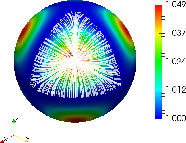
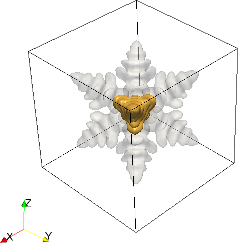
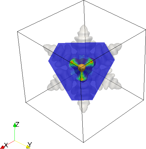
Figure 13: (a) Streamlines of $\boldsymbol{\mathcal{N}}^{\prime}$ (white lines) indicate that growth can occur in three directions which correspond to the secondary growing directions observed on (b). At the same time $t=1.5\times 10^{5}\delta t$, (c) $a_{s}(\mathbf{n})$ function is plotted in the plane of normal vector $\mathbf{n}_{d}=(1,\,1,\,1)^{T}$ centered at $\mathbf{x}_{p}=(331,\,244,\,244)^{T}$. $a_{s}$ is maximal in the same three directions.

Previous simulations were performed with a seed initialized at the center of the domain. Nevertheless, with this way to proceed, the dendrite is influenced by the domain boundaries before its full development. One first method consists to increase the computational domain by increasing the number of nodes. However, because 3D simulations require a lot of time computations, symmetries of problem are considered by keeping the same mesh. For dendrite B, the seed is initialized at the origin $(0,\,0,\,0)$ of the domain composed of $351^{3}$ nodes and the results are post-processed at the end of simulation. For that simulation, the 3D code calculates in parallel on 50 cores. The global domain is cut in $z$-direction for both equations. Each core calculates on a thin part of the global mesh composed of $351\times 351\times 7$ nodes. For $1.5\times 10^{5}$ times steps, the results are obtained after 98.54 hours ($\sim 4$ days). For comparison, results of Figs. 11(a), (b), (c) are respectively obtained after 3h, 8.97h and 9.18h for calculations on 100 cores.

The full dendrite is obtained by symmetry with respect to the planes $XY$, $YZ$ and $XZ$. In the simulation, the undercooling is $\Delta=0.25$ and parameters of $a_{s}(\mathbf{n})$ are $\varepsilon_{s}=0$ and $\gamma=-0.02$. The evolution of the dendritic structure $\phi=0$ is presented on Fig. 14 for six different times. A same orientation of the coordinate system was set for each figure.

(a) $t=0$		(b) $t=5\times 10^{3}\delta t$		(c) $t=1.5\times 10^{4}\delta t$
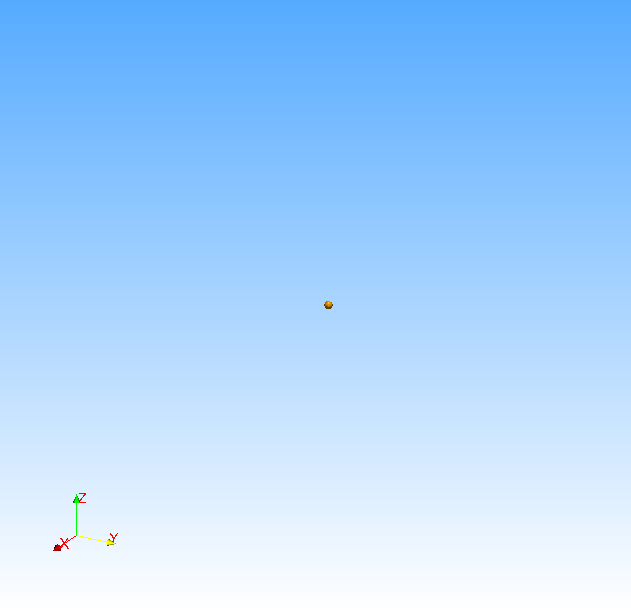
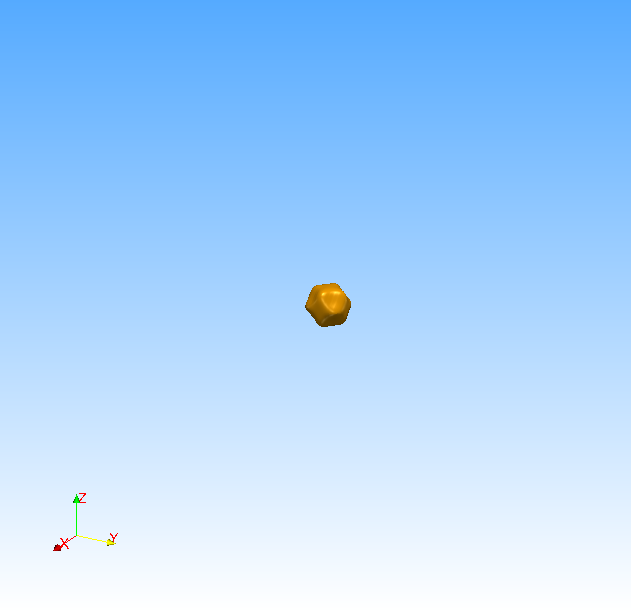
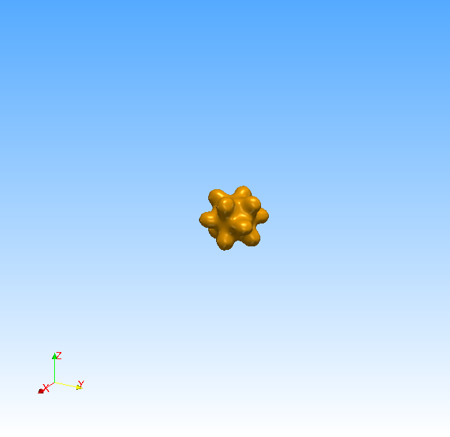
(d) $t=4\times 10^{4}\delta t$		(e) $t=10^{5}\delta t$		(f) $t=1.5\times 10^{5}\delta t$

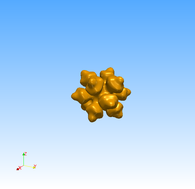
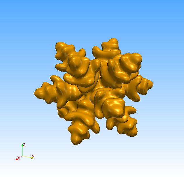
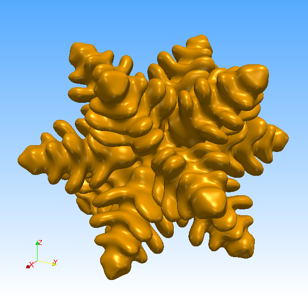
Figure 14: Phase-field evolution for $a_{s}(\mathbf{n})$ defined by Eq. (12) with $\varepsilon_{s}=0$ and $\gamma=-0.02$. The parameters are $W_{0}=0.0125$, $\tau_{0}=1.5625\times 10^{-4}$, $\lambda=10$, $\Delta=0.25$ and $\kappa=1$.

6 Conclusion

In this paper, the Lattice Boltzmann (LB) method, usually applied to simulate fluid flows, is applied to simulate crystal growth. The interface position and the temperature are modeled by a phase-field model which is numerically solved with a LB method. In this work, various dendritic shapes in 2D and 3D were simulated through the study of anisotropy function $a_{s}(\mathbf{n})$. That function is responsible for the anisotropic growth of crystals and appears in the phase-field equation.

A special care must be done when calculating the anisotropy function that involves the normal vector $\mathbf{n}$ of the interface. Indeed, for a sixfold symmetry in 2D, when a standard method of central finite differences is used to calculate $\mathbf{n}$, the phase-field $\phi=0$ is not any more isotropic. The solution does not match with itself after a rotation of 60° because a numerical anisotropy occurs on $a_{s}(\mathbf{n})$: the pattern of that function is not periodic. That lattice anisotropy can be decreased by using the Directional Derivatives (DD) method in order to compute the gradients. The number of directional derivatives is equal to the number of moving directions in the LB method. The gradient components are given by their moment of first order. Those directional derivatives are specific for each lattice and were used in this work for D2Q9 and D3Q15. The use of this method increases the accuracy of $a_{s}(\mathbf{n})$ and yields a pattern that is periodic. The solution is isotropic by rotation.

Next, the whole approach (LB+DD) was applied to simulate simultaneous growth of three crystals, each of them being defined by its own anisotropy function. For that purpose, a supplementary field $I(\mathbf{x},\,t)$ was added in the definition of $a_{s}$. That field carries the crystal number and evolves with the phase-field $\phi$. The method was applied for simulating in 2D the growth of three crystals with respectively four, five and six tips. Finally, several runs were performed with a 3D code for simulating standard and non standard dendrites. The anisotropy functions that have been used favor the growth in the $\left\langle 100\right\rangle$-, $\left\langle 110\right\rangle$- and $\left\langle 111\right\rangle$-directions. For each dendrite, the isotropy of the computational method was checked by carrying out several slices. After an appropriate rotation, the phase-fields are perfectly superimposed. For growth in the $\left\langle 111\right\rangle$-direction, the threefold symmetry of secondary branches is consistent with the $a_{s}(\mathbf{n})$ function. Indeed, the analysis of that function and its derivatives show that those secondary branches can appear in the three directions. This work shows the flexibility of the lattice Boltzmann method for simulating dendritic shapes defined by various anisotropy functions in 2D and 3D.

References

- Boettinger et al. [2002] W. J. Boettinger, J. A. Warren, C. Beckermann, A. Karma, Phase-Field Simulation of Solidification, Annual Review of Materials Research 32 (2002) pp. 163–194, doi:10.1146/annurev.matsci.32.101901.155803.
- Singer-Loginova and Singer [2008] I. Singer-Loginova, H. M. Singer, The phase field technique for modeling multiphase materials, Reports on Progress in Physics 71 (2008) 106501, doi:http://dx.doi.org/10.1088/0034-4885/71/10/106501.
- Steinbach [2009] I. Steinbach, Phase-field models in materials science, Modelling and Simulation in Materials Science and Engineering 17 (2009) pp. 1–31, doi:10.1088/0965-0393/17/7/073001.
- Provatas and Elder [2010] N. Provatas, K. Elder, Phase-Field Methods in Materials Science and Engineering, Wiley-VCH, ISBN: 978-3-527-40747-7, 2010.
- Kobayashi [1993] R. Kobayashi, Modeling and numerical simulations of dendritic crystal growth, Physica D 63 (1993) pp. 410–423, doi:10.1016/0167-2789(93)90120-P.
- Wang et al. [1993] S.-L. Wang, R. F. Sekerda, A. A. Wheeler, B. T. Murray, S. R. Coriell, R. J. Braun, G. B. McFadden, Thermodynamically-consistent phase-field models for solidification, Physica D 69 (1993) pp. 189–200, doi:10.1016/0167-2789(93)90189-8.
- Wheeler et al. [1993] A. A. Wheeler, B. T. Murray, R. J. Schaefer, Computation of dendrites using phase field model, Physica D 66 (1993) pp. 243–262, doi:10.1016/0167-2789(93)90242-S.
- Warren and Boettinger [1995] J. A. Warren, W. J. Boettinger, Prediction of dendritic growth and microsegregation patterns in a binary alloy using the phase-field method, Acta Metallurgica et Materiala 43 (2) (1995) pp. 689–703, doi:10.1016/0956-7151(94)00285-P.
- Kim et al. [1998] S. G. Kim, W. T. Kim, T. Suzuki, Interfacial compositions of solid and liquid in a phase-field model with finite interface thickness for isothermal solidification in binary alloys, Physical Review E 58 (3) (1998) pp. 3316–3323, doi:http://dx.doi.org/10.1103/PhysRevE.58.3316.
- Kim et al. [1999] S. G. Kim, W. T. Kim, T. Suzuki, Phase-field model for binary alloys, Physical Review E 60 (6) (1999) pp. 7186–7197, doi:http://dx.doi.org/10.1103/PhysRevE.60.7186.
- Karma and Rappel [1996a] A. Karma, W.-J. Rappel, Phase-field method for computationally efficient modeling of solidification with arbitrary interface kinetics, Physical Review E 53 (4) (1996a) R3017–R3020, doi:http://dx.doi.org/10.1103/PhysRevE.53.R3017.
- Karma and Rappel [1998] A. Karma, W.-J. Rappel, Quantitative phase-field modeling of dendritic growth in two and three dimensions, Physical Review E 57 (4) (1998) pp. 4323–4349, doi:http://dx.doi.org/10.1103/PhysRevE.57.4323.
- Anderson et al. [2000] D. M. Anderson, G. B. McFadden, A. A. Wheeler, A phase-field model of solidification with convection, Physica D 135 (2000) pp. 175–194, doi:10.1016/S0167-2789(99)00109-8.
- Bragard et al. [2002] J. Bragard, A. Karma, Y. H. Lee, M. Plapp, Linking Phase-Field and Atomistic Simulations to Model Dendritic Solidification in Highly Undercooled Melts, Interface Science 10 (2002) pp. 121–136, doi:10.1023/A:1015815928191.
- Echebarria et al. [2004] B. Echebarria, R. Folch, A. Karma, M. Plapp, Quantitative phase-field model of alloy solidification, Physical Review E 70 (061604) (2004) pp. 1–22, doi:http://dx.doi.org/10.1103/PhysRevE.70.061604.
- Ramirez et al. [2004] J. C. Ramirez, C. Beckermann, A. Karma, H.-J. Diepers, Phase-field modeling of binary alloy solidification with coupled heat and solute diffusion, Physical Review E 69 (051607) (2004) 1–16, doi:http://dx.doi.org/10.1103/PhysRevE.69.051607.
- Medvedev and Kassner [2005] D. Medvedev, K. Kassner, Lattice Boltzmann scheme for crystal growth in external flows, Physical Review E 72 (2005) 056703, doi:http://dx.doi.org/10.1103/PhysRevE.72.056703.
- Plapp [2007] M. Plapp, Three-dimensional phase-field simulations of directional solidification, Journal of Crystal Growth 303 (2007) pp. 49–57, doi:10.1016/j.jcrysgro.2006.12.064.
- Plapp [2011] M. Plapp, Unified derivation of phase-field models for alloy solidification from a grand-potential functional, Physical Review E 84 (031601) (2011) 1–15, doi:http://dx.doi.org/10.1103/PhysRevE.84.031601.
- Zhao et al. [2005] P. Zhao, J. Heinrich, D. Poirier, Dendritic solidification of binary alloys with free and forced convection, International Journal for Numerical Methods in Fluids 49 (2005) pp. 233–266, doi:10.1002/fld.988.
- Karma and Rappel [1996b] A. Karma, W.-J. Rappel, Numerical Simulation of Three-dimensional Dendritic Growth, Physical Review Letters 77 (19) (1996b) pp. 4050–4053, doi:http://dx.doi.org/10.1103/PhysRevLett.77.4050.
- Chen et al. [2009] C. C. Chen, Y. L. Tsai, C. W. Lan, Adaptative phase field simulation of dendritic crystal growth in a forced flow: 2D vs 3D morphologies, International Journal of Heat and Mass Transfer 52 (2009) pp. 1158–1166, doi:10.1016/j.ijheatmasstransfer.2008.09.014.
- Li et al. [2011] Y. Li, H. Lee, J. Kim, A fast, robust, and accurate operator splitting method for phase-field simulations of crystal growth, Journal of Crystal Growth 321 (2011) pp. 176–182, doi:10.1016/j.jcrysgro.2011.02.042.
- Bollada et al. [2015] P. Bollada, C. Goodyer, P. Jimack, A. Mullis, F. Yang, Three dimensional thermal-solute phase field simulation of binary alloy solidification, Journal of Computational Physics 287 (2015) pp. 130–150, doi:10.1016/j.jcp.2015.01.040.
- Nestler et al. [2005] B. Nestler, D. Danilov, P. Galenko, Crystal growth of pure substances: Phase-field simulations in comparison with analytical and experimental results, Journal of Computational Physics 207 (2005) pp. 221–239, doi:10.1016/j.jcp.2005.01.018.
- Chen and Doolen [1998] S. Chen, G. Doolen, Lattice Boltzmann Method for fluid flows, Annual Reviews of Fluid Mechanics 30 (1998) pp. 329–364, doi:10.1146/annurev.fluid.30.1.329.
- Succi [2001] S. Succi, The Lattice Boltzmann Equation for Fluid Dynamics and Beyond, Oxford Science Publication, 2001.
- Guo and Shu [2013] Z. Guo, C. Shu, Lattice Boltzmann Method and its Applications in Engineering, World Scientific Publishing Co. Pte. Ltd., 2013.
- Kendon et al. [2001] V. Kendon, M. Cates, I. Pagonabarraga, J.-C. Desplat, P. Bladon, Inertial effects in three-dimensional spinodal decomposition of a symmetric binary fluid mixture: a lattice Boltzmann study, Journal of Fluid Mechanics 440 (2001) pp. 147–203, doi:http://dx.doi.org/10.1017/S0022112001004682.
- Zheng et al. [2006] H. Zheng, C. Shu, Y. Chew, A lattice Boltzmann model for multiphase flows with large density ratio, Journal of Computational Physics 218 (2006) pp. 353–371, doi:10.1016/j.jcp.2006.02.015.
- Liu et al. [2014] H. Liu, A. Valocchi, C. Werth, Q. Kang, M. Oostrom, Pore-scale simulation of liquid CO2 displacement of water using a two-phase lattice Boltzmann model, Advances in Water Resources 73 (2014) pp. 144–158, doi:10.1016/j.advwatres.2014.07.010.
- Dellar [2002] P. Dellar, Lattice Kinetic Schemes for Magnetohydrodynamics, Journal of Computational Physics 179 (2002) pp. 95–126, doi:10.1006/jcph.2002.7044.
- Lin et al. [2014] G. Lin, J. Bao, Z. Xu, A three-dimensional phase field model coupled with a lattice kinetics solver for modeling crystal growth in furnaces with accelerated crucible rotation and traveling magnetic field, Computers & Fluids 103 (2014) pp. 204–214, doi:10.1016/j.compfluid.2014.07.027.
- Medvedev et al. [2006] D. Medvedev, T. Fischaleck, K. Kassner, Influence of external flows on crystal growth: Numerical investigation, Phsical Review E 74 (031606) (2006) 1–10, doi:http://dx.doi.org/10.1103/PhysRevE.74.031606.
- Chatterjee and Chakraborty [2006] D. Chatterjee, S. Chakraborty, A hybrid lattice Boltzmann model for solid-liquid phase transition in presence of fluid flow, Physics Letters A 351 (2006) pp. 359–367, doi:10.1016/j.physleta.2005.11.014.
- Rojas et al. [2015] R. Rojas, T. Takaki, M. Ohno, A phase-field-lattice Boltzmann method for modeling motion and growth of a dendrite for binary alloy solidification in the presence of melt convection, Journal of Computational Physics 298 (2015) pp. 29–40, doi:10.1016/j.jcp.2015.05.045.
- Rasin et al. [2005] I. Rasin, W. Miller, S. Succi, Phase-field lattice kinetics scheme for the numerical simulation of dendritic growth, Physical Review E 72 (066705) (2005) 1–8, doi:http://dx.doi.org/10.1103/PhysRevE.72.066705.
- Huber et al. [2008] C. Huber, A. Parmigiani, B. C. M. Manga, O. Bachmann, Lattice Boltzmann model for melting with natural convection, International Journal of Heat and Fluid Flow 29 (2008) pp. 1469–1480.
- Sun et al. [2009] D. Sun, M. Zhu, S. Pan, D. Raabe, Lattice Boltzmann modeling of dendritic growth in a forced melt convection, Acta Materialia 57 (2009) pp. 1755–1767.
- Miller and Succi [2002] W. Miller, S. Succi, A Lattice Boltzmann Model For Anisotropic Crystal Growth From Melt, Journal of Statistical Physics 107 (1/2) (2002) pp. 173–186, doi:10.1023/A:1014510704701.
- Miller et al. [2006] W. Miller, I. Rasin, S. Succi, Lattice Boltzmann phase-field modelling of binary-alloy solidification, Physica A 362 (2006) pp. 78–83, doi:10.1016/j.physa.2005.09.021.
- Jiaung et al. [2001] W.-S. Jiaung, J.-R. Ho, C.-P. Kuo, Lattice Boltzmann method for the heat conduction problem with phase change, Numerical Heat Transfer 39 (2001) pp. 167–187.
- Voller et al. [1987] V. Voller, M. Cross, N. Markatos, An enthalpy method for convection/diffusion phase change, International Journal for Numerical Methods in Engineering 24 (1987) 271–284.
- Brent et al. [1988] A. Brent, V. Voller, K. Reid, Enthalpy-porosity technique for modeling convection-diffusion phase change: application to the melting of a pure metal, Numerical Heat Transfer 13 (1988) 297–318.
- Kang et al. [2004] Q. Kang, D. Zhang, P. C. Lichtner, I. N. Tsimpanogiannis, Lattice Boltzmann model for crystal growth from supersaturated solution, Geophysical Research Letters 31 (2004) L21604, doi:10.1029/2004GL021107.
- Chen et al. [2014] L. Chen, Q. Kang, B. Carey, W.-Q. Tao, Pore-scale study of diffusion–reaction processes involving dissolution and precipitation using the lattice Boltzmann method, International Journal of Heat and Mass Transfer 75 (2014) pp. 483–496, http://dx.doi.org/10.1016/j.ijheatmasstransfer.2014.03.074.
- Min et al. [2016] T. Min, Y. Gao, L. Chen, Q. Kang, W.-Q. Tao, Mesoscale investigation of reaction–diffusion and structure evolution during Fe–Al inhibition layer formation in hot-dip galvanizing, International Journal of Heat and Mass Transfer 92 (2016) pp. 370–380, http://dx.doi.org/10.1016/j.ijheatmasstransfer.2015.08.083.
- Younsi et al. [2014] A. Younsi, A. Cartalade, M. Quintard, Lattice Boltzmann simulations for anisotropic crystal growth of a binary mixture, in: Proc. of The 15th International Heat Transfer Conference, 10-15 Aug. 2014, Kyoto, paper IHTC15-9797, ISBN: 978-1-56700-421-2, doi:10.1615/IHTC15.cpm.009797, 2014.
- Cartalade et al. [2016] A. Cartalade, A. Younsi, M. Plapp, Lattice Boltzmann simulations of 3D crystal growth: Numerical schemes for a phase-field model with anti-trapping current, Computers & Mathematics with Applications 71 (9) (2016) pp. 1784–1798, doi:10.1016/j.camwa.2016.02.029.
- Lee and Liu [2010] T. Lee, L. Liu, Lattice Boltzmann simulations of micron-scale drop impact on dry surfaces, Journal of Computational Physics 229 (2010) 8045–8063, doi:10.1016/j.jcp.2010.07.007.
- Lee and Fischer [2006] T. Lee, P. F. Fischer, Eliminating parasitic currents in the lattice Boltzmann equation method for non ideal gases, Physical Review E 74 (2006) 046709, doi:http://dx.doi.org/10.1103/PhysRevE.74.046709.
- Lee [2009] T. Lee, Effects of incompressibility on the elimination of parasitic currents in the lattice Boltzmann equation method for binary fluids, Computers and Mathematics with Applications 58 (2009) pp. 987–994, doi:10.1016/j.camwa.2009.02.017.
- Plapp and Karma [2000] M. Plapp, A. Karma, Multiscale Finite-Difference-Diffusion-Monte-Carlo Method for Simulating Dendritic Solidification, Journal of Computational Physics 165 (2000) pp. 592–619, doi:10.1006/jcph.2000.6634.
- Lin et al. [2011] H. Lin, C. Chen, C. Lan, Adaptive three-dimensional phase-field modeling of dendritic crystal growth with high anisotropy, Journal of Crystal Growth 318 (2011) pp. 51–54, doi:10.1016/j.jcrysgro.2010.11.013.
- Lu et al. [2005] Y. Lu, C. Beckermann, J. Ramirez, Three-dimensional phase-field simulations of the effect of convection on free dendritic growth, Journal of Crystal Growth 280 (2005) pp. 320–334, doi:10.1016/j.jcrysgro.2005.03.063.
- Dawson et al. [1993] S. P. Dawson, S. Chen, G. Doolen, Lattice Boltzmann computations for reaction-diffusion equations, Journal of Chemical Physics 98 (2) (1993) pp. 1514–1523, doi:http://dx.doi.org/10.1063/1.464316.
- Walsh and Saar [2010] S. Walsh, M. Saar, Macroscale lattice-Boltzmann methods for low Peclet number solute and heat transport in heterogeneous porous media, Water Resources Research 46 (W07517) (2010) 1–15, doi:10.1029/2009WR007895.
- d’Humières et al. [2002] D. d’Humières, I. Ginzburg, M. Krafczyk, P. Lallemand, L.-S. Luo, Multiple-relaxation-time lattice Boltzmann models in three dimensions, Phil. Trans. R. Soc. Lond. A 360 (2002) pp. 437–451, doi:10.1098/rsta.2001.0955.
- Ginzburg [2005] I. Ginzburg, Equilibrium-type and link-type lattice Boltzmann models for generic advection and anisotropic-dispersion equation, Advances in Water Resources 28 (2005) pp. 1171–1195, doi:http://dx.doi.org/10.1016/j.advwatres.2005.03.004.
- Yoshida and Nagaoka [2010] H. Yoshida, M. Nagaoka, Multiple-relaxation-time Lattice Boltzmann model for the convection and anisotropic diffusion equation, Journal of Computational Physics 229 (2010) pp. 7774–7795, doi:10.1016/j.jcp.2010.06.037.
- Cartalade et al. [2014] A. Cartalade, A. Younsi, É. Régnier, S. Schuller, Simulations of phase-field models for crystal growth and phase separation, Procedia Material Science 7 (2014) pp. 72–78, doi:10.1016/j.mspro.2014.10.010.
- Debierre et al. [2003] J.-M. Debierre, A. K. F. Celestini, R. Guerin, Phase-field approach for faceted solidification, Physical Review E 68 (041604) (2003) pp. 1–13.
- Miura [2013] H. Miura, Anisotropy function of kinetic coefficient for phase-field simulations: Reproduction of kinetic Wulff shape with arbitrary face angles, Journal of Crystal Growth 367 (2013) pp. 8–17, doi:10.1016/j.jcrysgro.2013.01.014.
- Fehlner and Vosko [1976] W. Fehlner, S. Vosko, A product representation for cubic harmonics and special directions for the determination of the Fermi surface and related properties, Canadian Journal of Physics 54 (1976) pp. 2159–2169.
- Mueller and Priestley [1966] F. Mueller, M. Priestley, Inversion of Cubic de Haas-van Alphen Data, with an Application to Palladium, Physical Review 148 (2) (1966) pp. 638–643.
- Puff [1970] H. Puff, Contribution to the Theory of Cubic Harmonics, Physica Status Solidi 41 (11) (1970) pp. 11–22.
- Hoyt et al. [2003] J. Hoyt, M. Asta, A. Karma, Atomistic and continuum modeling of dendritic solidification, Materials Science and Engineering: R: Reports 41 (6) (2003) pp. 121–163, doi:10.1016/S0927-796X(03)00036-6.
- Podmaniczky et al. [2014] F. Podmaniczky, G. Tóth, T. Pusztai, L. Gránásy, Free energy of the bcc–liquid interface and the Wulff shape as predicted by the phase-field crystal model, Journal of Crystal Growth 385 (2014) pp. 148–153, doi:10.1016/j.jcrysgro.2013.01.036.
- Haxhimali et al. [2006] T. Haxhimali, A. Karma, F. Gonzales, M. Rappaz, Orientation selection in dendritic evolution, Nature Materials 5 (2006) pp. 660–664, doi:10.1038/nmat1693.
- Dantzig et al. [2013] J. Dantzig, P. D. Napoli, J. Friedli, M. Rappaz, Dendritic Growth Morphologies in Al-Zn Alloys–Part II: Phase-Field Computations, Metallurgical and Materials Transactions A 44A (12) (2013) pp. 5532–5543, doi:10.1007/s11661-013-1911-8.