Spinning particles moving around black holes: integrability and chaos

Abstract

The motion of a stellar compact object around a supermassive black hole can be approximated by the motion of a spinning test particle. The equations of motion describing such systems are in general non-integrable, and therefore, chaotic motion should be expected. This article discusses the integrability issue of the spinning particle for the cases of Schwarzschild and Kerr spacetime, and then it focuses on a canonical Hamiltonian formalism where the spin of the particle is included only up to the linear order.

1 Introduction

The dynamics of a spinning particle moving in a curved spacetime background is of astrophysical interest as it approximates the motion of a stellar compact object moving around a supermassive black hole. The equation of motion of a spinning particle were provided by Mathisson [1] and Papapetrou [2]. However, the Mathisson-Papapetrou (MP) equations are less than the variables they intend to evolve. Thus, a spin supplementary condition (SSC) is required to close the system. There are aplenty SSCs (see, e.g., Refs. 3, 4 for a review), but, here we mention the Tulczyjew[5] (T) SSC and the Newton-Wigner[6] (NW) SSC.

The dynamical reason we are interested in the spinning particle motion is that chaos seems to appear for black hole backgrounds. Namely, it has been found that for the MP equations with T SSC chaotic motion is present in the case of a Schwarzschild background[7], and in the case of a Kerr background[8, 9]. However, it has been shown that when the MP equations with the T SSC are linearized, then a Carter-like integral of motion appears in the case of the Kerr background[10], which led some to argue that in the linearized in spin approach the MP equation correspond to an integrable system.

A case of a linearized in spin system approach was employed in order to get a canonical Hamiltonian formulation for the spinning particle system in Ref. 11. Namely, this formulation came from linearizing in spin the MP equations with the NW SSC. The Hamiltonian function for a Kerr background in Boyer-Linquist coordinates given in Ref. 11 suffers from several drawbacks[11, 13], and a revised Hamiltonian function in Boyer-Linquist coordinates has been provided in Ref. 12. By examining the latter function in the non-spinning limit of the central body, i.e., Schwarzschild, we have found that the system is integrable, while for the Kerr case chaos appears[13]. The appearance of chaos will be examined in detail in Ref. 14. In particular, in Ref. 14 we employ a 4D Poincaré method[15, 16] to investigate the dynamics of the spinning particle in the Hamiltonian approximation.

The article consists of the following sections. sec:eqm is a brief introduction to the canonical Hamiltonian formalism. sec:integr discusses the integrability issue of a spinning particle in black hole background. sec:Conc sums up the work.

2 Equations of motion

A canonical Hamiltonian formalism has been achieved by linearizing the MP equations of motion for the NW SSC[11]. The MP equations describe the motion of a particle with mass $m$ and spin $S^{\mu\nu}$ in a given spacetime background $g_{\mu\nu}$, i.e.,

$$\frac{D~{}p^{\mu}}{d\tau}=-\frac{1}{2}~{}{R^{\mu}}_{\nu\kappa\lambda}v^{\nu}S^{\kappa\lambda}~{}~{},~{}\frac{D~{}S^{\mu\nu}}{d\tau}=p^{\mu}~{}v^{\nu}-v^{\mu}~{}p^{\nu}~{}~{},$$ (1)

where ${R^{\mu}}_{\nu\kappa\lambda}$ is the Riemann tensor, $p^{\mu}$ is the four-momentum, $v^{\mu}=dx^{\mu}/d\tau$ is the four-velocity, and $\tau$ is the proper time. The NW SSC reads

$$S^{\mu\nu}~{}\omega_{\mu}=0~{}~{},$$ (2)

where $\omega_{\mu}$ is a sum of time-like vectors. This sum in our case[11] has the form

$$\omega_{\nu}=p_{\nu}-m~{}\tilde{e}_{\nu}^{~{}T}~{}~{},$$ (3)

where $\tilde{e}_{\nu}^{~{}T}$ is the timelike future oriented vector (T is used instead of 0), which together with three spacelike vectors $\tilde{e}^{\mu}_{I}$, is part of a tetrad field $\tilde{e}^{\mu}_{\Delta}$.

When a tensor is projected on the tetrad field, then it is denoted with capital indices. For example, $\omega_{\Delta}=\tilde{e}^{\nu}_{~{}\Delta}\omega_{\nu}$ is the projection of the time-like vector (3) on the tetrad field, i.e., $\omega_{T}=p_{\nu}~{}\tilde{e}^{\nu}_{T}-m,~{}\omega_{J}=p_{\nu}~{}\tilde{e}^{\nu}_{J}~{}.$ On the other hand, the spin tensor $S^{\mu\nu}$ projection reads $S^{IJ}=S^{\mu\nu}~{}\tilde{e}_{\mu}^{~{}I}~{}\tilde{e}_{\nu}^{~{}J}~{}.$ However, the Hamiltonian function of the spinning particle[11] does not use exactly the above described spin projection, instead employs the spin three vector $S_{I}=\frac{1}{2}\epsilon_{IJL}~{}S^{JL}~{},$ where $\epsilon_{IJL}$ is the Levi-Civita symbol.

Now, the Hamiltonian function $H$ for a spinning particle

$$H=H_{NS}+H_{S}~{}~{},$$ (4)

splits in two parts. The first

$$H_{NS}=\beta^{i}P_{i}+\alpha~{}\sqrt{m^{2}+\gamma^{ij}P_{i}P_{j}}$$ (5)

is the Hamiltonian for a non-spinning particle, where

$$\alpha=\frac{1}{\sqrt{-g^{00}}}~{}~{},~{}\beta^{i}=\frac{g^{0i}}{g^{00}}~{}~{},~{}\gamma^{ij}=g^{ij}-\frac{g^{0i}g^{0j}}{g^{00}}~{}~{},$$ (6)

and $P_{i}$ are the canonical momenta conjugate to $x^{i}$ of the Hamiltonian (4), which can be calculated from the “kinetic” momenta $p_{i}$ through the relation

$$P_{i}=p_{i}+E_{i\Gamma\Delta}S^{\Gamma\Delta}=p_{i}+\left(2E_{iTJ}\frac{\omega_{C}}{\omega_{T}}+E_{iJC}\right)\epsilon^{JCL}~{}S_{L}~{}~{},$$ (7)

where $E_{\nu\Gamma\Delta}=-\frac{1}{2}\left(g_{\kappa\lambda}~{}\tilde{e}^{\kappa}_{~{}\Gamma}~{}\frac{\partial\tilde{e}^{\lambda}_{~{}\Delta}}{\partial x^{\nu}}+\tilde{e}^{\kappa}_{~{}\Gamma}~{}\Gamma_{\kappa\nu\lambda}~{}\tilde{e}^{\lambda}_{~{}\Delta}\right)$ is a tensor which is antisymmetric in the last two indices, i.e., $E_{\nu\Gamma\Delta}=-E_{\nu\Delta\Gamma}$, and $\Gamma_{\kappa\nu\lambda}$ are the Christoffel symbols; the second part of the Hamiltonian

$$H_{S}=-\left(\beta^{i}F_{i}^{C}+F_{0}^{C}+\frac{\alpha~{}\gamma^{ij}P_{i}~{}F_{j}^{C}}{\sqrt{m^{2}+\gamma^{ij}P_{i}P_{j}}}\right)S_{C}$$ (8)

includes the spin of the particle, where $F_{\mu}^{C}=\left(2E_{\mu TI}\frac{\bar{\omega}_{J}}{\bar{\omega}_{T}}+E_{\mu IJ}\right)\epsilon^{IJC}$ and

$$\bar{\omega}_{\Delta}=\bar{\omega}_{\nu}~{}\tilde{e}^{\nu}_{~{}\Delta}~{}~{}, \bar{\omega}_{\nu}=\bar{P}_{\nu}-m~{}\tilde{e}_{\nu}^{~{}T}~{}~{}, \bar{P}_{i}=P_{i}~{}~{},$$

$$\bar{P}_{0}=-\beta^{i}~{}P_{i}-\alpha\sqrt{m^{2}+\gamma^{ij}P_{i}P_{j}}~{}~{}, \bar{\omega}_{T}=\bar{P}_{\nu}~{}\tilde{e}^{\nu}_{~{}T}-m~{}~{}, \bar{\omega}_{J}=\bar{P}_{\nu}~{}\tilde{e}^{\nu}_{~{}J}~{}~{}.$$ (9)

The equations of motion for the canonical variables as a function of coordinate time $t$ read

$$\frac{dx^{i}}{dt}=\frac{\partial H}{\partial P_{i}}~{}~{},\frac{dP_{i}}{dt}=-\frac{\partial H}{\partial x^{i}}~{}~{},\frac{dS_{I}}{dt}=\epsilon_{IJC}\frac{\partial H}{\partial S_{J}}S^{C}~{}~{}~{}~{}.$$ (10)

It should be noted that for the MP with NW SSC the mass $m=\sqrt{-p_{\nu}p^{\nu}}$ is not a constant of motion[11, 17]. However, in the procedure of linearizing in spin the MP equations to get the Hamiltonian approximation, $m$ becomes a constant of motion[11]. The explicit form of the revised Hamiltonian function for the Kerr spacetime in Boyer-Linquist coordinates can be found in Ref. 12; here the function is not presented, because it is lengthy.

3 The issue of integrability

When the particle is non-spinning then eq:MPeq gives the geodesic orbit, and the system is symplectic. In a symplectic system with each constant of motion the phase space can be reduced by two dimensions (one degree of freedom), while in a non-symplectic just by one dimension. In the case of a Kerr background for a geodesic orbit we have four integrals of motion, i.e., the mass of the particle, the energy, the component of the orbital angular momentum along the symmetry axis, and the Carter constant. The above integrals of motion are independent and in involution. For the geodesic motion we have 8 dimensional phase space (four degrees of freedom), therefore, the system is integrable.

By including the spin to the evolution scheme, we increase the dimensions of the phase space, and we break in general its symplectic structure. Namely, we have 4 dimensions from the position $x^{\mu}$, 4 from the velocities $v^{\mu}$, 4 from the momenta $p^{\mu}$, and 6 from the spin $S^{\mu\nu}$, so totally we have 18 dimensions. In the Kerr case from the Killing vectors we get 2 constants, but we lose the Carter constant. On the other hand in the Schwarzschild spacetime the Killing vectors provide 3 independent and in ivnolution constants. By including a SSC we get 3 independent constraints. For the MP with T SSC the measure of the particle’s spin is preserved, and the measure of the spin as well, so we have 2 constants more. The preservation of the four velocity is the last constant, which gives us in total for the Kerr 8 constants, while for the Schwarzschild 9 constants. But, since the system is not symplectic, the integrals are not enough to make the system integrable, and chaos appears both for the Schwarzschild[7] and for the Kerr[8, 9] background.

We need to linearize the MP equations in spin to decrease the dimensions, and to find new constants of motion. Namely, since the momenta and the velocities are parallel in the linear regime, the phase space decrease by 4, thus, we get a 14 dimensional phase space. A Carter like constant is regained for Kerr when the MP equations with T SSC are linearized in spin[10]. In the Schwarzschild limit the linearized in spin MP equations preserve the measure of the orbital angular momentum[18] for the Pirani SSC, which in the linear domain is the same with the T SSC. But, now the four-momentum contraction gives the same constant with the four-velocity contraction, thus we have one integral less.

In the Hamiltonian approximation the degrees of freedom are five, three come from the position variables, and two from the spin 3-vector. Thus, one needs five integrals of motion in order to have an integrable system. In the case of the Schwarzschild background we have the conservation of the total angular momentum giving two integrals, we have the conservation of the spin of the particle, since the system is autonomous the Hamiltonian function itself is a constant, and the measure of the orbital momentum is preserved as well[13]. Thus, the Hamiltonian approximation corresponds to an integrable system in the case of the Schwarzschild background[13] in contrast with the non-integrability of the MP equations with T SSC[7].

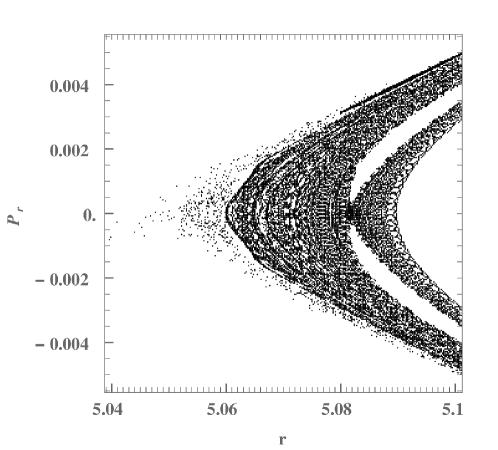
Figure 1: A detail from the surface of section lying on the equatorial plane. The basic parameters of the background spacetime are the mass $M=1$, and the spin $a=0.1$, while the particle’s basic parameters are $S=m=1$. $r$ is the radial distance in Boyer-Linquist coordinates, and $P_{r}$ the conjugate momentum For more details see Ref. 13.

However, the Hamiltonian approximation for Kerr appears to correspond to a non-integrable system in agreement with the full MP equations for T SSC[8, 9]. fig:2D shows a 2D surface of section, which is a projection of a 4D Poincaré section, for a slowly rotating central black hole $(a=0.1)$. The scattered dots in fig:2D show that chaos appears for the Hamiltonian function introduced in Ref. 12, which mean that the corresponding system is non-integrable. Moreover, the width of the KAM curves indicates that we have lost more than one integral when we turn on the spin of the central body. Since the azimuthal angular momentum, and the measure of the particle’s spin are still constant of motion. The system has 3 degrees of freedom. The non-appearance of the Carter-like constant for the revised Hamiltonian function implies either that the tetrad field suggested in Ref. 12 is not good, or that the Carter-like constant depends on the SSC we choose.

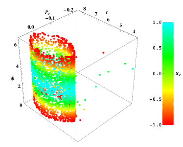
Figure 2: A 4D Poincaré section corresponding to two orbits from fig:2D. $\phi$ is the azimuthal angle. $S_{y}$ is one of the three components of the spin, and the coloring corresponds to its value as shown at the strips lying right of each section. The left panel corresponds to sticky chaotic orbit shown as scattered dots in fig:2D, while the right panel corresponds to a chain of stable islands corresponding to the two banana shaped white areas appearing at the right sight of fig:2D.

The 2D Poincaré section method is proper for systems of two degrees of freedom, when the system has three degrees of freedom the 2D surface of section is just a projection of a 4D Poincaré sections. 2D projections are useful tool to get a first feeling about the dynamics and have been used in the past[7, 8, 9]. However, in order to confirm what we are actually seeing, and to understand better the dynamics we need to use the 4D Poincaré sections[15, 16]. In fig:4D we show some preliminary results from a work in progress[14]. In this plot we present two 4D Poincaré sections, where the color plays the role of the fourth dimension. According to the color and rotation 4D Poincaré section method, the way an orbit evolves on a 3D projection along with the smoothness of the coloring shows whether an orbit is regular or chaotic[15, 16]. In the case of a chaotic orbit the orbit behaves irregularly on the 3D projection and/or the colors mix along its trajectory. In the case that a sticky chaotic orbit suffers from escapes like the case shown in fig:2D the only way to observe the chaotic nature of the orbit is not the mixing of colors but the (irregular) scattered points leaving the sticky zone (left panel of fig:4D). For an island of stability the regularity of the orbit is indeed shown by the toroidal structure of the islands and the smoothness of the color (right panel of fig:4D).

4 Conclusion

This article has discussed the issue of integrability for the case of the spinning particle, especially in the case when its dynamic is described by the canonical Hamiltonian linear in spin approximation. In the case of the Schwarzschild background, contrary to the non-integrability of the MP equations with T SSC[7], the Hamiltonian approximation corresponds to an integrable system[13]. While in the case of a Kerr background the non-integrability of the MP equations with T SSC[8, 9] is also the case for the revised Hamiltonian function[12]. The non-integrability of the latter is shown by a 2D surface of section[13], and by using the color and rotation 4D Poincaré section technique[14].

References

- [1] M. Mathisson, Acta Phys. Polonica 6, 163 (1937)
- [2] A. Papapetrou, Proc. R. Soc. London Ser. A 209, 248 (1951)
- [3] O. Semerák, Mon. Not. R. Astron. S. 308, 863 (1999)
- [4] K. Kyrian, and O. Semerák, Mon. Not. R. Astron. S. 382, 1922 (2007)
- [5] W. Tulczyjew, Acta Phys. Polonica 18, 393 (1959)
- [6] T. D. Newton and E. P. Wigner, Rev. Mod. Phys. 21, 400 (1949)
- [7] S. Suzuki and K. Maeda, Phys. Rev. D 55, 4848 (1997)
- [8] M. D. Hartl, Phys. Rev. D 67, 024005 (2003)
- [9] M. D. Hartl, Phys. Rev. D 67, 104023 (2003)
- [10] R. Rüdiger, Proc. R. Soc. London Ser. A 375, 185 (1981); 385, 229 (1982)
- [11] E. Barausse, E. Racine, and A. Buonanno, Phys. Rev. D 80, 104025 (2009)
- [12] E. Barausse, and A. Buonanno, Phys. Rev. D 81, 084024 (2010)
- [13] D. Kunst, T. Ledvinka, G. Lukes-Gerakopoulos, and J. Seyrich, Phys. Rev. D 93, 044004 (2016)
- [14] G. Lukes-Gerakopoulos, M. Katsanikas, P. Patsis and J. Seyrich, arXiv: 1606.09171, Phys. Rev. D (2016)
- [15] P. A. Patsis and L. Zachilas Int. J. Bif. Chaos 4, 1399-1424 (1994)
- [16] M. Katsanikas and P.A. Patsis Int. Journal Bif. Chaos 21, 467-496 (2011)
- [17] G. Lukes-Gerakopoulos, J. Seyrich, D. Kunst, Phys.Rev. D 90, 104019 (2014)
- [18] T. A. Apostolatos, Clas. Quant. Grav. 13, 799 (1996)
- [19] F. A. E. Pirani, Acta Phys. Polonica 15, 389 (1956)