Leading two-loop corrections to the Higgs boson masses in SUSY models with Dirac gauginos

Johannes Braathen,${}^{\!\!\!\,a,b}$  Mark D. Goodsell${}^{\,a,b}$  and Pietro Slavich${}^{\,a,b}$

^a LPTHE, UPMC Univ. Paris 06, Sorbonne Universités, 4 Place Jussieu, F-75252 Paris, France

^b LPTHE, CNRS, 4 Place Jussieu, F-75252 Paris, France

1 Introduction

In anticipation of new results from the run II of the LHC, supersymmetry (SUSY) as a framework remains the leading candidate for physics beyond the Standard Model (SM). However, the discovery of a SM-like Higgs boson with relatively large mass and the lack of observation of coloured superparticles have spurred considerable interest in SUSY realisations beyond the Minimal Supersymmetric Standard Model (MSSM). A notable extension beyond the minimal case is to allow Dirac masses for the gauginos [1, 2, 3, 4, 5, 6], in particular instead of – but possibly in addition to – Majorana ones. Among the reasons for the growing interest in this scenario are that Dirac gaugino masses relax constraints on squark masses (through suppressing production) [7, 8, 9] and flavour constraints [10, 11, 12], and that they increase the naturalness of the model (because the operators are supersoft [4] and the SM-like Higgs boson mass is enhanced at tree level [13, 14]).

Dirac gaugino masses require the addition of two fermionic degrees of freedom (i.e., an extra Weyl spinor) for each gaugino. We can then write a mass term that respects a global chiral symmetry, which in SUSY models is promoted to a global $U(1)$ $R$-symmetry. We also require the same number of extra scalar degrees of freedom as fermionic ones; this implies that after electroweak symmetry breaking (EWSB) we have four new neutral scalar degrees of freedom compared to the MSSM, which may mix with the neutral scalars of the Higgs sector. The new states are packaged in an adjoint chiral multiplet for each gauge group, which should also have couplings to the Higgs scalars, possibly enhancing the SM-like Higgs boson mass at both tree and loop level.

There is more than one way to construct a Dirac-gaugino extension of the MSSM. The minimal choice, which we will denote as the Minimal Dirac Gaugino Supersymmetric Standard Model (MDGSSM), consists in simply adding the adjoint chiral multiplets to the field content of the MSSM, and allowing for all gauge-invariant terms in the superpotential and in the soft SUSY-breaking Lagrangian. The reader should note that in recent works [15, 16, 17] the term MDGSSM has also been used to describe a unified scenario where extra lepton-like states are added to ensure natural gauge-coupling unification, but the distinction will be irrelevant for this paper.

If we wish to avoid large Majorana masses for the gauginos – and benefit from simpler SUSY-breaking scenarios [18] – we should avoid $R$-symmetry breaking in the soft terms, which also means removing the MSSM-like $A$-terms; this then naturally embeds into gauge-mediated scenarios [6, 19, 20, 21, 22, 23, 24]. We may retain a $B_{\mu}$ term since it is required for EWSB and will not generate Majorana masses through renormalisation group evolution. The variant without a $\mu$ term is called $\not{\mu}$SSM or $\mu$-less MSSM [5], and can be considered a special case of this model (note that, as studied in ref. [25], the $\not{\mu}$SSM is currently challenged by electroweak precision measurements).

On the other hand, if we choose to retain the $R$-symmetry as exact (possibly broken only by gravitational effects) then one popular construction is the Minimal $R$-symmetric Supersymmetric Standard Model, or MRSSM [10]: two additional Higgs-like superfields are included, which couple in the superpotential to the regular Higgs doublets but obtain no expectation value. They allow the Higgs fields $H_{u}$ and $H_{d}$ to both have zero $R$-charge and contribute to EWSB without violating the $R$-symmetry. An even more minimal realisation is the MMRSSM [26, 27], where the down-type Higgs $H_{d}$ and its $R$-partner are missing, a sneutrino then playing the role of $H_{d}$. Another option to preserve $R$-symmetry is the supersymmetric one-Higgs-doublet model [28]: starting from the field content of the MDGSSM, the singlet adjoint superfield is missing and the down-type Higgs does not develop an expectation value, therefore the bino is massless up to anomaly-mediation contributions.

The extended Higgs sectors of these theories have an interesting and varied phenomenology. From past experience in the study of the Higgs sector of the MSSM and of the Next-to-Minimal Supersymmetric Standard Model (NMSSM), we expect the radiative corrections to the Higgs boson masses in Dirac-gaugino models to be crucial to obtain a reasonable precision and rule in/out scenarios, or assess their naturalness. For the MSSM, the corrections to the Higgs boson masses have been computed at two loops in the limit of vanishing external momenta [29, 30, 31, 32, 33, 34, 35, 36, 37, 38, 39, 40, 41, 42], and the dominant momentum-dependent two-loop corrections [43, 44, 45] as well as the dominant three-loop corrections [46, 47, 48] have also been obtained. For the NMSSM, beyond the one-loop level only the two-loop corrections involving the strong gauge coupling together with the top or bottom Yukawa couplings, usually denoted as ${\cal O}(\alpha_{t}\alpha_{s})$ and ${\cal O}(\alpha_{b}\alpha_{s})$, have been computed [49, 50]. In contrast, in other supersymmetric extensions of the SM there have been no explicit calculations of the Higgs masses beyond one-loop results.

On the other hand, the public tool SARAH [51, 52, 53, 54, 55, 56] can, for a generic supersymmetric model, automatically compute the full one-loop corrections to all particle masses, as well as the two-loop corrections to the neutral-scalar masses in the limit of vanishing electroweak gauge couplings and external momenta [57, 58], implementing and extending the general two-loop results of refs. [59, 60]. Recently, SARAH has made it possible to analyse at the two-loop level the Higgs sector of several non-minimal extensions of the MSSM, see refs. [61, 62, 63, 64, 65]. Of particular relevance for this work, it has allowed for Dirac-gaugino masses since version 3.2 [54], incorporating also the results of ref. [66]. Indeed, SARAH has been used for detailed phenomenological analyses of the MDGSSM at one loop in ref. [25] and at two loops in refs. [15, 16]; and also for the MRSSM at one loop in ref. [67] and two loops in refs. [68, 69].

However, while such a numerical tool for generic models fulfils a significant need of the community, it is also important to have explicit results for specific models, and not just as a cross-check. In this work we shall compute the leading ${\cal O}(\alpha_{t}\alpha_{s})$ corrections to the neutral Higgs boson masses in both the MDGSSM and MRSSM, relying on the effective-potential techniques developed in ref. [36] for the MSSM and in ref. [49] for the NMSSM. This has the following advantages:

• We compute the ${\cal O}(\alpha_{t}\alpha_{s})$ corrections in both the ${\overline{\rm DR}}$ and on-shell (OS) renormalisation schemes. The latter turns out to be particularly useful in scenarios with heavy gluinos – a feature of many Dirac-gaugino models in the literature – where the use of ${\overline{\rm DR}}$ formulae for the two-loop Higgs-mass corrections can lead to large theoretical uncertainties.

• We have written a simple and fast stand-alone code implementing our results, which we make available upon request (indeed, a version of the code is already included in SARAH).

• We use our results to derive simple approximate expressions for the most important two-loop corrections, applicable in any Dirac gaugino model.

The outline of the paper is as follows. In section 2 we define the important parameters of our theory. In section 3 we present our results for the general case, the MDGSSM and the MRSSM, show how we compute the shift to the OS scheme, and give simplified formulae for the SM-like Higgs boson mass either for a common SUSY-breaking scale or for a heavy Dirac gluino. In section 4 we give numerical examples of our results, illustrating the advantages of our approach and also discussing the inherent theoretical uncertainties. We conclude in section 5. Explicit expressions for the derivatives of the effective potential are given in an appendix.

2 Definition of the theory

2.1 Adjoint multiplets and the supersoft operator

In order to give gauginos a Dirac mass it is necessary to pair each Weyl fermion of the vector multiplets with another Weyl fermion $\chi_{\Sigma}$ in the adjoint representation of the gauge group. These adjoint fermions sit inside chiral superfields, which we shall denote collectively $\mathbf{\Sigma}^{a}\,=\,\Sigma^{a}\,+\,\sqrt{2}\,\theta\chi^{a}_{\Sigma}\,+\ldots\,$, where the lowest-order component $\Sigma^{a}$ is a complex scalar. In models with softly-broken supersymmetry, the Dirac gaugino mass arises only in the supersoft operator:

$$\mathcal{L}_{\mathrm{supersoft}} = \int d^{2}\theta\,\sqrt{2}\,m_{D}\,\theta^{\alpha}\,\mathbf{W}_{\alpha}^{a}\,\mathbf{\Sigma}^{a}~{}+~{}{\rm h.c.}$$ (2.1)

$$\supset -m_{D}\,\lambda^{a}\chi^{a}_{\Sigma}~{}+~{}\sqrt{2}\,m_{D}\,\Sigma^{a}\,D^{a}\ ~{}+~{}{\rm h.c.},$$

where $\mathbf{W}_{\alpha}^{a}\,=\,\lambda^{a}_{\alpha}\,+\,\theta_{\alpha}D^{a}\,+\ldots$ is the field-strength superfield. Integrating out the auxiliary field $D^{a}$ leads to mass terms for the adjoint scalars, as well as to trilinear interactions between the adjoint scalars and the MSSM-like scalars, which we collectively denote as $\phi$:

$$\mathcal{L}~{}\supset~{}-(m_{D}\,\Sigma^{a}+m_{D}^{*}\,\Sigma^{a\,*})^{2}-\sqrt{2}\,g\,(m_{D}\,\Sigma^{a}+m_{D}^{*}\,\Sigma^{a\,*})\,\phi^{*}\,t^{a}\,\phi~{},$$ (2.2)

where $t^{a}$ are the generators of the gauge group in the representation appropriate to $\phi$, and a sum over the gauge indices of $\phi$ is understood. Considering all sources of mass terms for the adjoint scalars,

$$\mathcal{L}~{}\supset~{}-(m_{\Sigma}^{2}+2\,|m_{D}|^{2})\,\Sigma^{a\,*}\Sigma^{a}-\frac{1}{2}\,(B_{\Sigma}+2\,m_{D}^{2})\,\Sigma^{a}\,\Sigma^{a}-\frac{1}{2}\,(B_{\Sigma}^{*}+2\,m_{D}^{*\,2})\,\Sigma^{a\,*}\Sigma^{a\,*}~{},$$ (2.3)

where $m_{\Sigma}^{2}$ includes in general contributions from both the superpotential and the soft SUSY-breaking Lagrangian, and $B_{\Sigma}$ is a soft SUSY-breaking bilinear term. In addition, mixing with the MSSM-like Higgs scalars may be induced, upon EWSB, by the $D$-term interactions in eq. (2.2), as well as by superpotential interactions.

We shall denote the adjoint multiplet for $U(1)_{Y}$ as a singlet $\mathbf{S}=S\,+\,\sqrt{2}\,\theta\chi_{S}\,+\ldots\,$, the one for $SU(2)_{L}$ as a triplet $\mathbf{T}^{a}=T^{a}\,+\,\sqrt{2}\,\theta\chi_{T}^{a}\,+\ldots\,$, and the one for $SU(3)$ as an octet $\mathbf{O}^{a}=O^{a}+\sqrt{2}\,\theta\chi_{O}^{a}\,+\ldots\,$. In this paper we shall be interested only in the two-loop corrections to the Higgs masses involving the strong gauge coupling $g_{s}$, thus the relevant trilinear couplings in eq. (2.2) will be the ones involving the octet scalar and the squarks.

We shall make the additional restriction that the octet scalar only interacts via the strong gauge coupling and the above trilinear terms, equivalent to the assumption that it has no superpotential couplings or soft trilinear couplings other than with itself. This shall simplify the computations, and it is true for almost all variants of Dirac gaugino models studied so far. To have renormalisable Yukawa couplings between the octet and the MSSM fields we would need to add new coloured states (such as a vector-like top). However, in the most general version of the MDGSSM there could also be terms that violate the above assumption – which have only recently attracted attention [71, 17] – namely couplings between the singlet and the octet of the form

$$W~{}\supset~{}\frac{1}{2}\,\lambda_{SO}\,\mathbf{S}\,\mathbf{O}^{a}\mathbf{O}^{a},\qquad\mathcal{L}~{}\supset~{}-\frac{1}{2}\,T_{SO}\,S\,O^{a}O^{a}\,+\,{\rm h.c.}~{}.$$ (2.4)

The coupling $\lambda_{SO}$ is typically neglected because it violates $R$-symmetry and leads to Majorana gaugino masses: for example, in the restricted version of the MDGSSM or the $\not{\mu}SSM$ the $R$-symmetry violation is assumed to only occur in the Higgs sector and possibly only via gravitational effects. On the other hand, there is no symmetry preventing the generation of $T_{SO}$, but it is typically difficult for it to obtain a phenomenologically significant magnitude, hence it has been neglected – see [17] for a full discussion (and for cases when it could be large). Furthermore, $T_{SO}$ is irrelevant in the decoupling limit (when the singlet $S$ is heavy) that we shall employ later in our simplified formulae.

With the above assumptions, we can make a rotation of the superfield $\mathbf{O}^{a}$ such that we can take $m_{D}$ to be real without loss of generality, but we cannot simultaneously require that the soft SUSY-breaking bilinear $B_{O}$ be real without additionally imposing CP invariance. The octet mass terms are then

$$\mathcal{L}~{}\supset~{}-m_{O}^{2}\,O^{a\,*}O^{a}~{}-~{}\frac{1}{2}\,B_{O}\,O^{a}\,O^{a}~{}-~{}\frac{1}{2}\,B_{O}^{*}\,O^{a\,*}O^{a\,*}-m_{D}^{2}\,(O^{a}+O^{a\,*})^{2}~{}.$$ (2.5)

If $B_{O}$ is not real, the real and imaginary parts of the octet scalar mix with each other. Their mass matrix can be diagonalised with a rotation by an angle $\phi_{O}\,$,

$$O^{a}~{}=~{}\frac{e^{i\phi_{O}}}{\sqrt{2}}\,(O_{1}^{a}+i\,O_{2}^{a})~{},~{}~{}~{}~{}~{}~{}~{}~{}\phi_{O}~{}=~{}-\frac{1}{2}\,{\rm Arg}\left(B_{O}+2\,m_{D}^{2}\right)~{},$$ (2.6)

to obtain the two mass eigenvalues

$$m^{2}_{O_{1,2}}~{}=~{}m_{O}^{2}+2\,m_{D}^{2}\pm|2\,m_{D}^{2}+B_{O}|~{}.$$ (2.7)

Then the trilinear couplings of the octet mass eigenstates $O^{a}_{1,2}$ to squarks $\tilde{q}_{L}$ and $\tilde{q}_{R}$ read

$$\mathcal{L}~{}\supset~{}-2\,g_{s}\,m_{D}\,(\cos\phi_{O}\,O_{1}^{a}-\sin\phi_{O}\,O_{2}^{a})~{}(\tilde{q}_{L}^{*}\,t^{a}\,\tilde{q}_{L}-\tilde{q}_{R}^{*}\,t^{a}\,\tilde{q}_{R})~{},$$ (2.8)

where $t^{a}$ are the generators of the fundamental representation of $SU(3)$. These couplings lead to new (compared to MSSM and NMSSM) contributions to the two-loop effective potential involving the octet scalars which will affect the Higgs masses. We remark that, since in eq. (2.5) the superpotential mass term $m_{D}^{2}$ affects only the real part of the octet scalar, the mixing angle $\phi_{O}$ is suppressed by $m_{D}^{2}$ in the limit where the latter is much larger than the soft SUSY-breaking mass terms. In particular,

$$\cos\phi_{O}~{}\approx~{}1~{}+~{}{\cal O}\left(m_{D}^{-4}\right)~{},~{}~{}~{}~{}~{}~{}~{}~{}~{}~{}\sin\phi_{O}~{}\approx~{}-\frac{{\rm Im}(B_{O})}{4\,m_{D}^{2}}~{}+~{}{\cal O}\left(m_{D}^{-4}\right)~{}.$$ (2.9)

For the remainder of this paper, we shall restrict our attention to the CP-conserving case. This is motivated by clarity and simplicity in the calculations, and also physically in that there are strong constraints upon CP violation, even in the Higgs sector[72, 73, 74, 75]. However, we shall make an exception in allowing a non-zero angle $\phi_{O}$, because it is particularly simple to do so, and its effects are only felt at an order beyond that considered here: it generates CP-violating phases in the stop mass matrix at two loops, and in the Higgs mass at three. This is because the couplings in eq. (2.8) are real, and phases only appear in the octet scalar-gluino-gluino vertex.

2.2 Gluino masses and couplings

In the case of Dirac gauginos, there is mixing between the Weyl fermion of the gauge multiplet $\lambda^{a}$ and its Dirac partner $\chi^{a}_{\Sigma}$. We shall allow in general both Majorana and Dirac masses which, in two-component notation, we write as

$$\mathcal{L}~{}\supset~{}-\,\frac{1}{2}\,M_{\lambda}\,\lambda^{a}\lambda^{a}\,-\,\frac{1}{2}\,M_{\Sigma}\,\chi^{a}_{\Sigma}\chi^{a}_{\Sigma}\,-\,m_{D}\,\lambda^{a}\chi^{a}_{\Sigma}\,+\,{\rm h.c.}~{}.$$ (2.10)

As mentioned in the previous section, we can define $m_{D}$ to be real. In general we cannot remove the phases from both $M_{\lambda}$ and $M_{\Sigma}$; however, as also mentioned above, we shall not consider CP violation in the gluino sector, and thus take all three masses to be real. We then rotate $\lambda^{a}$ and $\chi^{a}_{\Sigma}$ to mass eigenstates $\lambda^{a}_{1}$ and $\lambda^{a}_{2}$ via a mixing matrix $R_{ij}$, so that

$$\lambda^{a}~{}=~{}R_{11}\,\lambda^{a}_{1}\,+\,R_{12}\,\lambda^{a}_{2}\,,\qquad\chi^{a}_{\Sigma}~{}=~{}R_{21}\,\lambda^{a}_{1}\,+\,R_{22}\,\lambda_{2}^{a}~{}.$$ (2.11)

In four-component notation, this leads in general to two Majorana gauginos with different masses. In case of a pure Dirac mass, however, we obtain two Majorana gauginos with degenerate masses $|m_{\lambda_{1}}|=|m_{\lambda_{2}}|=|m_{D}|\,$, which can also be combined in a single Dirac gaugino.

We recall that in the models of interest in this paper there are no Yukawa couplings of the additional octet superfield, therefore the two gluino mass-eigenstates only couple to quarks and squarks via their gaugino component $\lambda^{a}$. In particular, the couplings of each (four-component) gluino $\tilde{g}^{a}_{i}$ are simply related to the couplings of the usual (N)MSSM gluino by an insertion of the mixing matrix:

$$\mathcal{L}~{}\supset~{}-\sqrt{2}\,g_{s}\,R_{1i}\,\left[\,\tilde{q}_{L}^{*}\,t^{a}\,(\overline{\tilde{g}^{a}_{i}}\,P_{L}\,q)\,-\,(\overline{q}\,P_{L}\,\tilde{g}^{a}_{i})\,t^{a}\,\tilde{q}_{R}\,\right]~{}+~{}{\rm h.c.}~{},$$ (2.12)

where a sum over the $SU(3)$ indices of quarks and squarks is again understood. Consequently, as we shall see below, the gluino contribution to the two-loop effective potential in Dirac-gaugino models can be trivially recovered from the known results valid in the MSSM and in the NMSSM.

2.3 Higgs sector

We now consider the Higgs sector of the theory. Dirac gaugino models extend the (N)MSSM, so we shall assume that we have at least the usual two Higgs doublets $H_{u}$ and $H_{d}$. To these we must add the adjoint scalars $S$ and $T^{a}$ mentioned above, which mix with the Higgs fields. The couplings of the adjoint scalars, as well as the presence of any additional fields in the Higgs sector, will, however, depend on the model under consideration. In the following we shall focus on the minimal Dirac-gaugino extension of the MSSM, the MDGSSM, and on the minimal $R$-symmetric extension, the MRSSM.

In the MDGSSM there are no additional superfields apart from the adjoint ones, and the superpotential reads

$$W = W_{\mathrm{Yukawa}}\,+\,W_{\mathrm{MDGSSM}}~{},$$ (2.13)

$$W_{\mathrm{Yukawa}} = Y_{u}^{ij}\,\mathbf{U}_{i}\mathbf{Q}_{j}\cdot\mathbf{H_{u}}\,-\,Y_{d}^{ij}\,\mathbf{D}_{i}\mathbf{Q}_{j}\cdot\mathbf{H_{d}}\,-\,Y_{e}^{ij}\,\mathbf{E}_{i}\mathbf{L}_{j}\cdot\mathbf{H_{d}}~{},$$ (2.14)

$$W_{\mathrm{MDGSSM}} = (\mu+\lambda_{S}\,\mathbf{S})\,\mathbf{H_{u}}\cdot\mathbf{H_{d}}\,+\,\lambda_{T}\,\mathbf{H_{d}}\cdot\mathbf{T}^{a}\,\sigma^{a}\,\mathbf{H_{u}}\,+\,W_{\Sigma}~{},$$ (2.15)

where $\sigma^{a}$ are Pauli matrices, and the dot-product denotes the antisymmetric contraction of the $SU(2)_{L}$ indices. In addition to the terms explicitly shown in eqs. (2.14) and (2.15), the most general renormalisable superpotential contains terms involving only the adjoint superfields – namely, mass terms for each of them, all trilinear terms allowed by the gauge symmetries, and a linear term for the singlet – which we denote collectively as $W_{\Sigma}$. The most general soft SUSY-breaking Lagrangian for the MDGSSM contains non-holomorphic mass terms for all of the scalars, as well as Majorana mass terms for the gauginos, plus $A$-type (i.e., trilinear), $B$-type (i.e., bilinear) and tadpole (i.e., linear) holomorphic terms for the scalars with the same structure as the terms in the superpotential. With the assumption, discussed in section 2.1, that we neglect the couplings $\lambda_{SO}$ and $T_{SO}$ defined in eq. (2.4), the superpotential $W_{\Sigma}$ and the soft SUSY-breaking terms that involve only the adjoint fields are not relevant to the calculation of the two-loop ${\cal O}(\alpha_{t}\alpha_{s})$ corrections to the Higgs masses presented in this paper, apart from contributing to the masses and mixing of the adjoint fields as discussed in sections 2.1 and 2.2 above.

In the case of the MRSSM, we must add two superfields $\mathbf{R_{u}}$ and $\mathbf{R_{d}}$ with the same gauge quantum numbers as $\mathbf{H_{d}}$ and $\mathbf{H_{u}}$, respectively, but with different charges under a conserved $R$-symmetry. The superpotential reads

$$W = W_{\mathrm{Yukawa}}\,+\,W_{\mathrm{MRSSM}}~{},$$ (2.16)

$$W_{\mathrm{MRSSM}} = (\mu_{d}+\lambda_{S_{d}}\,\mathbf{S})\,\mathbf{R_{d}}\cdot\mathbf{H_{d}}\,+\,\lambda_{T_{d}}\,\mathbf{H_{d}}\cdot\mathbf{T}^{a}\,\sigma^{a}\,\mathbf{R_{d}}$$ (2.17)

$$+ (\mu_{u}+\lambda_{S_{u}}\,\mathbf{S})\,\mathbf{H_{u}}\cdot\mathbf{R_{u}}\,+\,\lambda_{T_{u}}\,\mathbf{R_{u}}\cdot\mathbf{T}^{a}\,\sigma^{a}\,\mathbf{H_{u}}~{},$$

while all terms involving only the MSSM-like Higgs superfields and/or the adjoint superfields, such as those in eq. (2.15), are forbidden by the $R$-symmetry. The most general soft SUSY-breaking Lagrangian for the MRSSM contains non-holomorphic mass terms for all of the scalars, plus all of the holomorphic terms involving only the MSSM-like Higgs scalars and/or the adjoint scalars (which, as mentioned above, have no equivalent in the superpotential). In contrast, the $R$-symmetry forbids Majorana mass terms for the gauginos, and holomorphic terms for the scalars with the same structure as the terms in the MRSSM superpotential. The requirement that the $R$-symmetry is conserved also means that the scalar doublets $R_{u}$ and $R_{d}$ do not develop a vacuum expectation value (vev), and do not mix with either the MSSM-like Higgs scalars or the adjoint scalars.

3 Two-loop corrections in the effective potential approach

In this section we adapt to the calculation of two-loop corrections to the neutral Higgs masses in Dirac-gaugino models the effective-potential techniques developed in ref. [36] for the MSSM and in ref. [49] for the NMSSM. We start by deriving general results valid for all variants of Dirac-gaugino extensions of the MSSM, then we provide explicit formulae for the MDGSSM and MRSSM models discussed in section 2.

3.1 General results

The effective potential for the neutral Higgs sector can be decomposed as $V_{\mathrm{eff}}=V_{0}+\Delta V$, where $\Delta V$ incorporates the radiative corrections. We denote collectively as $\Phi_{i}^{0}$ the complex neutral scalars whose masses we want to calculate, and split them into vacuum expectation values $v_{i}$, real scalars $S_{i}$ and pseudoscalars $P_{i}$ as

$$\Phi_{i}^{0}~{}\equiv~{}v_{i}+\frac{1}{\sqrt{2}}(S_{i}+i\,P_{i})~{}.$$ (3.1)

Then the mass matrices for the scalar and pseudoscalar fields can be decomposed as

$$\left({\cal M}^{2}_{S}\right)^{\rm eff}_{ij}~{}=~{}\left({\cal M}^{2}_{S}\right)^{\rm tree}_{ij}+\left(\Delta{\cal M}^{2}_{S}\right)_{ij}~{},~{}~{}~{}~{}~{}~{}~{}~{}~{}~{}\left({\cal M}^{2}_{P}\right)^{\rm eff}_{ij}~{}=~{}\left({\cal M}^{2}_{P}\right)^{\rm tree}_{ij}+\left(\Delta{\cal M}^{2}_{P}\right)_{ij}~{},$$ (3.2)

and the radiative corrections to the mass matrices are

$$\left(\Delta{\cal M}^{2}_{S}\right)_{ij} = -\frac{1}{\sqrt{2}}\,\frac{\delta_{ij}}{v_{i}}\left.\frac{\partial\Delta V}{\partial S_{i}}\right|_{\rm min}~{}+~{}\left.\frac{\partial^{2}\Delta V}{\partial S_{i}\partial S_{j}}\right|_{\rm min}~{},$$ (3.3)

$$\left(\Delta{\cal M}^{2}_{P}\right)_{ij} = -\frac{1}{\sqrt{2}}\,\frac{\delta_{ij}}{v_{i}}\left.\frac{\partial\Delta V}{\partial S_{i}}\right|_{\rm min}~{}+~{}\left.\frac{\partial^{2}\Delta V}{\partial P_{i}\partial P_{j}}\right|_{\rm min}~{},$$ (3.4)

where $v_{i}$, which we assume to be real, denote the vevs of the full radiatively-corrected potential $V_{\mathrm{eff}}$, and the derivatives are in turn evaluated at the minimum of the potential. The single-derivative terms in eqs. (3.3) and (3.4) arise when the minimum conditions of the potential,

$$\left.\frac{\partial V_{\mathrm{eff}}}{\partial S_{i}}\right|_{\rm min}=~{}0~{},$$ (3.5)

are used to remove the soft SUSY-breaking mass for a given field $\Phi_{i}^{0}$ from the tree-level parts of the mass matrices. It is understood that those terms should be omitted for fields that do not develop a vev (such as, e.g., the fields $R_{u,d}$ in the MRSSM).

With a straightforward application of the chain rule for the derivatives of the effective potential, the mass-matrix corrections in eqs. (3.3) and (3.4) and the minimum conditions in eq. (3.5) can be computed by exploiting the Higgs-field dependence of the parameters appearing in $\Delta V$. We restrict for simplicity our calculation to the so-called “gaugeless limit”, i.e. we neglect all corrections controlled by the electroweak gauge couplings $g$ and $g^{\prime}$. At the two-loop level, we focus on the contributions to $\Delta V$ from top/stop loops that involve the strong interactions. In Dirac-gaugino models, this results in corrections to mass matrices and minimum conditions that are proportional to $\alpha_{s}$ times various combinations of the top Yukawa coupling $y_{t}$ with the superpotential couplings of the singlet and triplet fields. It is therefore with a slight abuse of notation that we maintain the MSSM-inspired habit of denoting collectively those corrections as ${\cal O}(\alpha_{t}\alpha_{s})$.

As detailed in refs. [36, 49], if we neglect the electroweak contributions to the stop mass matrix the parameters in the top/stop sector depend on the neutral Higgs fields only through two combinations, which we denote as $X\equiv|X|\,e^{i\varphi}$ and $\widetilde{X}\equiv|\widetilde{X}|\,e^{i\tilde{\varphi}}$. They enter the stop mass matrix as

$$\mathcal{M}^{2}_{\mathrm{stop}}~{}=~{}\left(\begin{array}[]{cc}m_{Q}^{2}+|X|^{2}&\widetilde{X}^{*}\\ \widetilde{X}&m_{U}^{2}+|X|^{2}\end{array}\right)~{},$$ (3.6)

where $m_{Q}^{2}$ and $m_{U}^{2}$ are the soft SUSY-breaking mass terms for the stops. While $X=y_{t}\,H_{u}^{0}$ both in the (N)MSSM and in Dirac-gaugino models, the precise form of $\widetilde{X}$ depends on the model under consideration and will be discussed later. For the time being, we only assume that $\widetilde{X}$ is real at the minimum of the potential, to prevent CP-violating contributions to the Higgs mass matrices. The top/stop ${\cal O}(\alpha_{s})$ contribution to $\Delta V$ can then be expressed in terms of five field-dependent parameters, which can be chosen as follows. The squared top and stop masses

$$m_{t}^{2}=|X|^{2}~{},~{}~{}~{}~{}~{}~{}~{}m^{2}_{\tilde{t}_{1,2}}=\frac{1}{2}\left[(m_{Q}^{2}+m_{U}^{2}+2\,|X|^{2}\,)\pm\sqrt{(m_{Q}^{2}-m_{U}^{2})^{2}+4\,|\widetilde{X}|^{2}}\,\right]~{},$$ (3.7)

a mixing angle $\bar{\theta}_{\tilde{t}}$, with $0\leq\bar{\theta}_{\tilde{t}}\leq\pi/2$, which diagonalises the stop mass matrix after the stop fields have been redefined to make it real and symmetric

$$\sin 2\,\bar{\theta}_{\tilde{t}}=\frac{2\,|\widetilde{X}|}{m_{\tilde{t}_{1}}^{2}-m_{\tilde{t}_{2}}^{2}}~{},$$ (3.8)

and a combination of the phases of $X$ and $\widetilde{X}$ that we can choose as

$$\cos\,(\varphi-\tilde{\varphi})=\frac{{\rm Re}(\widetilde{X})\,{\rm Re}(X)+{\rm Im}(\widetilde{X})\,{\rm Im}(X)}{|\widetilde{X}|\,|X|}~{}.$$ (3.9)

Finally, the gluino masses $m_{\tilde{g}_{i}}$ and the octet masses $m_{O_{i}}^{2}$ do not depend on the Higgs background, since we neglect the singlet-octet couplings $\lambda_{SO}$ and $T_{SO}$. In the following we will also refer to $\theta_{t}$, with $-\pi/2<\theta_{t}<\pi/2$, i.e. the usual field-independent mixing angle that diagonalises the stop mass matrix at the minimum of the scalar potential.

We find general expressions for the top/stop contributions to the minimum conditions of the effective potential and to the corrections to the scalar and pseudoscalar mass matrices:

$$\left.\frac{\partial\Delta V}{\partial S_{i}}\right|_{\rm min} = s_{2\theta_{t}}\,\frac{\partial\widetilde{X}}{\partial S_{i}}\,F~{}+~{}\sqrt{2}\,y_{t}\,m_{t}\,\delta_{i2}\,G~{},$$ (3.10)

$$\Big{(}\Delta\mathcal{M}_{S}^{2}\Big{)}_{ij} = \bigg{(}s_{2\theta_{t}}\,\frac{\partial^{2}\widetilde{X}}{\partial S_{i}\partial S_{j}}+\frac{2}{m_{\tilde{t}_{1}}^{2}-m_{\tilde{t}_{2}}^{2}}\,\frac{\partial\widetilde{X}}{\partial S_{i}}\,\frac{\partial\widetilde{X}}{\partial S_{j}}\,-\frac{s_{2\theta_{t}}}{\sqrt{2}}\,\frac{\delta_{ij}}{v_{i}}\,\frac{\partial\widetilde{X}}{\partial S_{j}}\bigg{)}\,F$$

$$+ \!\!\!2\,y_{t}^{2}\,m_{t}^{2}\,\delta_{i2}\delta_{j2}\,F_{1}+\sqrt{2}\,m_{t}\,y_{t}\,s_{2\theta_{t}}\bigg{(}\delta_{i2}\frac{\partial\widetilde{X}}{\partial S_{j}}\,+\delta_{j2}\frac{\partial\widetilde{X}}{\partial S_{i}}\bigg{)}\,F_{2}+s_{2\theta_{t}}^{2}\,\frac{\partial\widetilde{X}}{\partial S_{i}}\,\frac{\partial\widetilde{X}}{\partial S_{j}}\,F_{3}\,,$$

$$\Big{(}\Delta\mathcal{M}_{P}^{2}\Big{)}_{ij} = \bigg{(}\frac{1}{m_{\tilde{t}_{1}}^{2}-m_{\tilde{t}_{2}}^{2}}\frac{\partial^{2}|\widetilde{X}|^{2}}{\partial P_{i}\partial P_{j}}-\frac{s_{2\theta_{t}}}{\sqrt{2}}\,\frac{\delta_{ij}}{v_{i}}\,\frac{\partial\widetilde{X}}{\partial S_{j}}\bigg{)}\,F$$ (3.12)

$$+ \bigg{(}\frac{\delta_{i2}}{v_{2}}\,\widetilde{X}+\sqrt{2}\,i\,\frac{\partial\widetilde{X}}{\partial P_{i}}\bigg{)}\bigg{(}\frac{\delta_{j2}}{v_{2}}\,\widetilde{X}+\sqrt{2}\,i\,\frac{\partial\widetilde{X}}{\partial P_{j}}\bigg{)}\,\tan\beta\,F_{\varphi}~{},$$

where all quantities are understood as evaluated at the minimum of the potential, no summation is implied over repeated indices, the fields are ordered as $(\Phi_{1}^{0}\,,\Phi_{2}^{0}\,,\,...)=(H_{d}^{0}\,,H_{u}^{0}\,,\,...)\,$, and again the terms involving $\delta_{ij}/v_{i}$ should be omitted if $\Phi_{i}^{0}$ does not develop a vev. The angle $\beta$ is defined as in the MSSM by $\tan\beta=v_{2}/v_{1}$. Here and thereafter we also adopt the shortcuts $c_{\phi}\equiv\cos\phi$ and $s_{\phi}\equiv\sin\phi$ for a generic angle $\phi$. The functions $F,G,F_{1},F_{2},F_{3}$ and $F_{\varphi}$ entering eqs. (3.10)–(3.12) are combinations of the derivatives of $\Delta V$. Explicit expressions for most of those functions can be found e.g. in ref. [49], but we display all of them here for completeness:

$$F = \frac{\partial\Delta V}{\partial m_{\tilde{t}_{1}}^{2}}-\frac{\partial\Delta V}{\partial m_{\tilde{t}_{2}}^{2}}-\frac{4\,c_{2\theta_{t}}^{2}}{m_{\tilde{t}_{1}}^{2}-m_{\tilde{t}_{2}}^{2}}\,\frac{\partial\Delta V}{\partial c_{2\bar{\theta}_{t}}^{2}}~{},$$ (3.13)

$$G = \frac{\partial\Delta V}{\partial m_{t}^{2}}+\frac{\partial\Delta V}{\partial m_{\tilde{t}_{1}}^{2}}+\frac{\partial\Delta V}{\partial m_{\tilde{t}_{2}}^{2}}~{},$$ (3.14)

$$F_{1} = \frac{\partial^{\,2}\Delta V}{(\partial m_{t}^{2})^{2}}+\frac{\partial^{\,2}\Delta V}{(\partial m_{\tilde{t}_{1}}^{2})^{2}}+\frac{\partial^{\,2}\Delta V}{(\partial m_{\tilde{t}_{2}}^{2})^{2}}+2\,\frac{\partial^{\,2}\Delta V}{\partial m_{t}^{2}\partial m_{\tilde{t}_{1}}^{2}}+2\,\frac{\partial^{\,2}\Delta V}{\partial m_{t}^{2}\partial m_{\tilde{t}_{2}}^{2}}+2\,\frac{\partial^{\,2}\Delta V}{\partial m_{\tilde{t}_{1}}^{2}\partial m_{\tilde{t}_{2}}^{2}}~{},$$ (3.15)

$$F_{2} = \frac{\partial^{\,2}\Delta V}{(\partial m_{\tilde{t}_{1}}^{2})^{2}}-\frac{\partial^{\,2}\Delta V}{(\partial m_{\tilde{t}_{2}}^{2})^{2}}+\frac{\partial^{\,2}\Delta V}{\partial m_{t}^{2}\partial m_{\tilde{t}_{1}}^{2}}-\frac{\partial^{\,2}\Delta V}{\partial m_{t}^{2}\partial m_{\tilde{t}_{2}}^{2}}$$ (3.16)

$$-\frac{4\,c_{2\theta_{t}}^{2}}{m_{\tilde{t}_{1}}^{2}-m_{\tilde{t}_{2}}^{2}}\left(\frac{\partial^{\,2}\Delta V}{\partial c_{2\bar{\theta}_{t}}^{2}\partial m_{t}^{2}}+\frac{\partial^{\,2}\Delta V}{\partial c_{2\bar{\theta}_{t}}^{2}\partial m_{\tilde{t}_{1}}^{2}}+\frac{\partial^{\,2}\Delta V}{\partial c_{2\bar{\theta}_{t}}^{2}\partial m_{\tilde{t}_{2}}^{2}}\right)~{},$$

$$F_{3} = \frac{\partial^{\,2}\Delta V}{(\partial m_{\tilde{t}_{1}}^{2})^{2}}+\frac{\partial^{\,2}\Delta V}{(\partial m_{\tilde{t}_{2}}^{2})^{2}}-2\,\frac{\partial^{\,2}\Delta V}{\partial m_{\tilde{t}_{1}}^{2}\partial m_{\tilde{t}_{2}}^{2}}-\frac{2}{m_{\tilde{t}_{1}}^{2}-m_{\tilde{t}_{2}}^{2}}\left(\frac{\partial\Delta V}{\partial m_{\tilde{t}_{1}}^{2}}-\frac{\partial\Delta V}{\partial m_{\tilde{t}_{2}}^{2}}\right)$$

$$+\frac{16\,c_{2\theta_{t}}^{2}}{(m_{\tilde{t}_{1}}^{2}-m_{\tilde{t}_{2}}^{2})^{2}}\,\left(c_{2\theta_{t}}^{2}\,\frac{\partial^{\,2}\Delta V}{(\partial c_{2\bar{\theta}_{t}}^{2})^{2}}+2\,\frac{\partial\Delta V}{\partial c_{2\bar{\theta}_{t}}^{2}}\right)-\frac{8\,c_{2\theta_{t}}^{2}}{m_{\tilde{t}_{1}}^{2}-m_{\tilde{t}_{2}}^{2}}\,\left(\frac{\partial^{\,2}\Delta V}{\partial c_{2\bar{\theta}_{t}}^{2}\partial m_{\tilde{t}_{1}}^{2}}-\frac{\partial^{\,2}\Delta V}{\partial c_{2\bar{\theta}_{t}}^{2}\partial m_{\tilde{t}_{2}}^{2}}\right)~{},$$

$$F_{\varphi} = -\frac{2\,z_{t}\,\cot\beta}{s_{2\theta_{t}}^{2}\,(m_{\tilde{t}_{1}}^{2}-m_{\tilde{t}_{2}}^{2})^{2}}\,\frac{\partial\Delta V}{\partial c_{\varphi_{t}-\tilde{\varphi}_{t}}}~{},$$ (3.18)

where we defined $z_{t}\equiv{\rm sign}(\widetilde{X}|_{\rm min})$.

3.2 Two-loop top/stop contributions to the effective potential

For the computation of the two-loop ${\cal O}(\alpha_{t}\alpha_{s})$ corrections to the Higgs mass matrices in models with Dirac gauginos we need the explicit expression for the top/stop ${\cal O}(\alpha_{s})$ contribution to $\Delta V$, expressed in terms of the field-dependent parameters defined in the previous section. In addition to the contributions of diagrams involving gluons, gluinos or the D-term-induced quartic stop couplings, which are in common with the (N)MSSM and can be found in ref. [36], $\Delta V$ receives a contribution from the diagram shown in figure 1, involving stops and octet scalars.

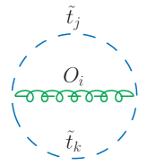
Figure 1: Novel two-loop contribution to the effective potential involving stops and octet scalars.

We assume that the gaugino masses are real so that the diagonalising matrix $R_{ij}$ is real and $R_{1i}^{2}$ is positive, but allow $m_{\tilde{g}_{i}}$ to be negative. Since $R_{11}^{2}+R_{12}^{2}=1$, we can simply write the top/stop ${\cal O}(\alpha_{s})$ contribution to the two-loop effective potential (in units of $\alpha_{s}\,C_{F}N_{c}\,/(4\pi)^{3}$, where $C_{F}=4/3$ and $N_{c}=3$ are colour factors) as

$$\Delta V^{\,\alpha_{s}}~{}=~{}\sum_{i=1}^{2}\,R_{1i}^{2}\,\Delta V^{\,\alpha_{s}}_{{\rm{\scriptscriptstyle MSSM}}}\,+~{}~{}\Delta V^{\,\alpha_{s}}_{\rm octet}~{},$$ (3.19)

where $\Delta V^{\,\alpha_{s}}_{{\rm{\scriptscriptstyle MSSM}}}$ is the analogous contribution in the (N)MSSM,

$$\Delta V^{\,\alpha_{s}}_{{\rm{\scriptscriptstyle MSSM}}} = 2\,J(m_{t}^{2},m_{t}^{2})-4\,m_{t}^{2}\,I(m_{t}^{2},m_{t}^{2},0)+$$ (3.20)

$$+ \biggr{\{}2\,m_{\tilde{t}_{1}}^{2}\,I(m_{\tilde{t}_{1}}^{2},m_{\tilde{t}_{1}}^{2},0)+2\,L(m_{\tilde{t}_{1}}^{2},m_{\tilde{g}_{i}}^{2},m_{t}^{2})-4\,m_{t}\,m_{\tilde{g}_{i}}\,s_{2\bar{\theta}}\,c_{\varphi-\tilde{\varphi}}\,I(m_{\tilde{t}_{1}}^{2},m_{\tilde{g}_{i}}^{2},m_{t}^{2})$$

$$+\,\frac{1}{2}\,(1+c_{2\bar{\theta}}^{2})\,J(m_{\tilde{t}_{1}}^{2},m_{\tilde{t}_{1}}^{2})+\frac{s_{2\bar{\theta}}^{2}}{2}J(m_{\tilde{t}_{1}}^{2},m_{\tilde{t}_{2}}^{2})\;\;+\;\;\left[m_{\tilde{t}_{1}}\leftrightarrow m_{\tilde{t}_{2}}\,,\,s_{2\bar{\theta}}\rightarrow-s_{2\bar{\theta}}\right]\biggr{\}},~{}~{}~{}$$

while $\Delta V^{\,\alpha_{s}}_{\rm octet}$ is the additional ${\cal O}(\alpha_{s})$ contribution of the two-loop diagram shown in figure 1, involving stops and octet scalars. The latter can be decomposed as

$$\Delta V^{\,\alpha_{s}}_{\rm octet}~{}\equiv~{}m_{D}^{2}\,\left(c_{\phi_{O}}^{2}\Delta V_{O_{1}}~{}+~{}s_{\phi_{O}}^{2}\Delta V_{O_{2}}\right)~{},$$ (3.21)

with

$$\Delta V_{O_{i}}~{}=~{}-2\,c_{2\bar{\theta}_{t}}^{2}\,\left[I(m_{\tilde{t}_{1}}^{2},m_{\tilde{t}_{1}}^{2},m_{O_{i}}^{2})\,+\,I(m_{\tilde{t}_{2}}^{2},m_{\tilde{t}_{2}}^{2},m_{O_{i}}^{2})\right]\,-\,4\,s_{2\bar{\theta}_{t}}^{2}\,I(m_{\tilde{t}_{1}}^{2},m_{\tilde{t}_{2}}^{2},m_{O_{i}}^{2})~{}.$$ (3.22)

The two-loop integrals $J(x,y)$, $I(x,y,z)$ and $L(x,y,z)$ entering eqs. (3.20) and (3.22) are defined, e.g., in eqs. (D1)–(D3) of ref. [49], and were first introduced in ref. [76]. Explicit expressions for the derivatives of $\Delta V^{\,\alpha_{s}}$, valid for all Dirac-gaugino models considered in this paper, are provided in appendix A.

We remark that, by using the “minimally subtracted” two-loop integrals of ref. [76], we are implicitly assuming a ${\overline{\rm DR}}$ renormalisation for the parameters entering the tree-level and one-loop parts of the effective potential. Consequently, our results for the two-loop top/stop contributions to mass matrices and minimum conditions also assume that the corresponding tree-level and one-loop parts are expressed in terms of ${\overline{\rm DR}}$-renormalised parameters. We will describe in section 3.5 how our two-loop formulae should be modified if the top/stop parameters entering the one-loop part of the corrections are expressed in a different renormalisation scheme. For what concerns the parameters entering the tree-level mass matrices for scalars and pseudoscalars – whose specific form depends on the Dirac-gaugino model under consideration – they can be taken directly as ${\overline{\rm DR}}$-renormalised inputs at some reference scale $Q$, at least in the absence of any experimental information on an extended Higgs sector. Exceptions are given by the electroweak gauge couplings and by the combination of doublet vevs $v\equiv(v_{1}^{2}+v_{2}^{2})^{1/2}\,$, which in general should be extracted from experimentally known observables such as, e.g., the muon decay constant and the gauge-boson masses. As was pointed out for the NMSSM in ref. [50], the extraction of the ${\overline{\rm DR}}$ parameter $v(Q)$ involves two-loop corrections whose effects on the scalar and pseudoscalar mass matrices are formally of the same order as some of the ${\cal O}(\alpha_{t}\alpha_{s})$ corrections computed in this paper. However, a two-loop determination of $v(Q)$ goes beyond the scope of our calculation, as it requires two-loop contributions to the gauge-boson self-energies which cannot be obtained with effective-potential methods. Besides, ref. [50] showed that, at least in the NMSSM scenarios considered in that paper, the ${\cal O}(\alpha_{t}\alpha_{s})$ effects on the scalar masses arising from the two-loop corrections to $v$ are quite small, typically of the order of a hundred MeV.

3.3 Mass corrections in the MDGSSM

The MDGSSM contains a singlet $S$ and an $SU(2)$ triplet $T^{a}$ which mix with the usual Higgs fields $H_{d}$ and $H_{u}$. In this model, the stop mixing term $\widetilde{X}$ defined in eq. (3.6) reads

$$\widetilde{X}~{}=~{}y_{t}\,\biggr{(}A_{t}\,H_{u}^{0}-\mu\,H_{d}^{0\,*}-\lambda_{S}\,S^{*}\,H_{d}^{0\,*}-\lambda_{T}\,T^{0\,*}\,H_{d}^{0\,*}\biggr{)}~{},$$ (3.23)

where $A_{t}$ is the soft SUSY-breaking trilinear interaction term for Higgs and stops. We order the neutral components of the fields as $\Phi_{i}^{0}=(H_{d}^{0},\,H_{u}^{0},\,S,\,T^{0})$ and expand them as in eq. (3.1). For the minimum conditions of the effective potential, eq. (3.10) gives

$$\left.\frac{\partial\Delta V}{\partial S_{1}}\right|_{\rm min} = -y_{t}\,\frac{\tilde{\mu}}{\sqrt{2}}\,s_{2\theta_{t}}\,F~{},$$ (3.24)

$$\left.\frac{\partial\Delta V}{\partial S_{2}}\right|_{\rm min} = \sqrt{2}\,y_{t}\,m_{t}\,G~{}+~{}y_{t}\,\frac{A_{t}}{\sqrt{2}}\,s_{2\theta_{t}}\,F~{},$$ (3.25)

$$\left.\frac{\partial\Delta V}{\partial S_{3}}\right|_{\rm min} = -y_{t}\,\frac{\lambda_{S}\,v_{1}}{\sqrt{2}}\,s_{2\theta_{t}}\,F~{},$$ (3.26)

$$\left.\frac{\partial\Delta V}{\partial S_{4}}\right|_{\rm min} = -y_{t}\,\frac{\lambda_{T}\,v_{1}}{\sqrt{2}}\,s_{2\theta_{t}}\,F~{},$$ (3.27)

where we defined $\tilde{\mu}\,\equiv\,\mu+\lambda_{S}\,v_{3}+\lambda_{T}\,v_{4}$. For the corrections to the mass matrices of scalars and pseudoscalars, eqs. (3.1) and (3.12) give

$$\Big{(}\Delta\mathcal{M}^{2}_{S}\Big{)}_{11} = \frac{1}{2}\,y_{t}^{2}\,\tilde{\mu}^{2}\,s_{2\theta_{t}}^{2}\,F_{3}~{}+~{}\frac{y_{t}^{2}\,A_{t}\,\tilde{\mu}\,\tan\beta}{m_{\tilde{t}_{1}}^{2}-m_{\tilde{t}_{2}}^{2}}\,F~{},$$ (3.28)

$$\Big{(}\Delta\mathcal{M}^{2}_{S}\Big{)}_{12} = -\,y_{t}^{2}\,m_{t}\,\tilde{\mu}\,s_{2\theta_{t}}\,\,F_{2}~{}-~{}\frac{1}{2}\,y_{t}^{2}\,A_{t}\,\tilde{\mu}\,s_{2\theta_{t}}^{2}\,F_{3}~{}-\,\frac{y_{t}^{2}\,A_{t}\,\tilde{\mu}}{m_{\tilde{t}_{1}}^{2}-m_{\tilde{t}_{2}}^{2}}\,F~{},$$ (3.29)

$$\Big{(}\Delta\mathcal{M}^{2}_{S}\Big{)}_{22} = 2\,y_{t}^{2}\,m_{t}^{2}\,F_{1}~{}+~{}2\,y_{t}^{2}\,m_{t}\,A_{t}\,s_{2\theta_{t}}\,F_{2}~{}+~{}\frac{1}{2}\,y_{t}^{2}\,A_{t}^{2}\,s_{2\theta_{t}}^{2}\,F_{3}~{}+\,\frac{y_{t}^{2}A_{t}\,\tilde{\mu}\,\cot\beta}{m_{\tilde{t}_{1}}^{2}-m_{\tilde{t}_{2}}^{2}}\,F~{},$$ (3.30)

$$\Big{(}\Delta\mathcal{M}^{2}_{S}\Big{)}_{13} = \frac{1}{2}\,y_{t}\,\lambda_{S}\,m_{t}\,\tilde{\mu}\,\cot\beta\,s_{2\theta_{t}}^{2}\,F_{3}~{}-\,\frac{y_{t}\,\lambda_{S}\,m_{t}\,\Big{(}A_{t}-2\,\tilde{\mu}\,\cot\beta\Big{)}}{m_{\tilde{t}_{1}}^{2}-m_{\tilde{t}_{2}}^{2}}\,F~{},$$ (3.31)

$$\Big{(}\Delta\mathcal{M}^{2}_{S}\Big{)}_{23} = \!\!-y_{t}\,\lambda_{S}\,m_{t}^{2}\,\cot\beta\,s_{2\theta_{t}}\,F_{2}-\frac{1}{2}\,y_{t}\,\lambda_{S}\,A_{t}\,m_{t}\cot\beta\,s_{2\theta_{t}}^{2}\,F_{3}-\frac{y_{t}\,\lambda_{S}\,m_{t}\,A_{t}\,\cot\beta}{m_{\tilde{t}_{1}}^{2}-m_{\tilde{t}_{2}}^{2}}\,F,$$ (3.32)

$$\Big{(}\Delta\mathcal{M}^{2}_{S}\Big{)}_{33} = \frac{1}{2}\,\lambda_{S}^{2}\,m_{t}^{2}\,{\cot}^{2}\beta\,s_{2\theta_{t}}^{2}\,F_{3}~{}+~{}\,\frac{\lambda_{S}\,m_{t}^{2}\,\cot\beta\,\Big{(}A_{t}+(\lambda_{S}\,v_{3}-\tilde{\mu})\cot\beta\Big{)}}{v_{3}\,(m_{\tilde{t}_{1}}^{2}-m_{\tilde{t}_{2}}^{2})}\,F~{},$$ (3.33)

$$\Big{(}\Delta\mathcal{M}^{2}_{S}\Big{)}_{14} = \frac{1}{2}\,y_{t}\,\lambda_{T}\,m_{t}\,\tilde{\mu}\,\cot\beta\,s_{2\theta_{t}}^{2}\,F_{3}~{}-\,\frac{y_{t}\,\lambda_{T}\,m_{t}\,\Big{(}A_{t}-2\,\tilde{\mu}\,\cot\beta\Big{)}}{m_{\tilde{t}_{1}}^{2}-m_{\tilde{t}_{2}}^{2}}\,F~{},$$ (3.34)

$$\Big{(}\Delta\mathcal{M}^{2}_{S}\Big{)}_{24} = \!\!-y_{t}\,\lambda_{T}\,m_{t}^{2}\,\cot\beta\,s_{2\theta_{t}}\,F_{2}-\frac{1}{2}\,y_{t}\,\lambda_{T}\,A_{t}\,m_{t}\cot\beta\,s_{2\theta_{t}}^{2}\,F_{3}-\frac{y_{t}\,\lambda_{T}\,m_{t}\,A_{t}\,\cot\beta}{m_{\tilde{t}_{1}}^{2}-m_{\tilde{t}_{2}}^{2}}\,F,$$ (3.35)

$$\Big{(}\Delta\mathcal{M}^{2}_{S}\Big{)}_{34} = \frac{1}{2}\,\lambda_{S}\,\lambda_{T}\,m_{t}^{2}\,{\cot}^{2}\beta\,s_{2\theta_{t}}^{2}\,F_{3}~{}+\,\frac{\lambda_{S}\,\lambda_{T}\,m_{t}^{2}\,{\cot}^{2}\beta}{m_{\tilde{t}_{1}}^{2}-m_{\tilde{t}_{2}}^{2}}\,F~{},$$ (3.36)

$$\Big{(}\Delta\mathcal{M}^{2}_{S}\Big{)}_{44} = \frac{1}{2}\,\lambda_{T}^{2}\,m_{t}^{2}\,{\cot}^{2}\beta\,s_{2\theta_{t}}^{2}\,F_{3}~{}+~{}\,\frac{\lambda_{T}\,m_{t}^{2}\,\cot\beta\,\Big{(}A_{t}+(\lambda_{T}\,v_{4}-\tilde{\mu})\cot\beta\Big{)}}{v_{4}\,(m_{\tilde{t}_{1}}^{2}-m_{\tilde{t}_{2}}^{2})}\,F~{},$$ (3.37)

$$\Big{(}\Delta\mathcal{M}^{2}_{P}\Big{)}_{11} = \frac{y_{t}^{2}\,A_{t}\,\tilde{\mu}\,\tan\beta}{m_{\tilde{t}_{1}}^{2}-m_{\tilde{t}_{2}}^{2}}\,F~{}+~{}y_{t}^{2}\,\tilde{\mu}^{2}\,\tan\beta\,F_{\varphi}~{},$$ (3.38)

$$\Big{(}\Delta\mathcal{M}^{2}_{P}\Big{)}_{12} = \frac{y_{t}^{2}\,A_{t}\,\tilde{\mu}}{m_{\tilde{t}_{1}}^{2}-m_{\tilde{t}_{2}}^{2}}\,F~{}+~{}y_{t}^{2}\,\tilde{\mu}^{2}\,F_{\varphi}~{},$$ (3.39)

$$\Big{(}\Delta\mathcal{M}^{2}_{P}\Big{)}_{22} = \frac{y_{t}^{2}\,A_{t}\,\tilde{\mu}\,\cot\beta}{m_{\tilde{t}_{1}}^{2}-m_{\tilde{t}_{2}}^{2}}\,F~{}+~{}y_{t}^{2}\,\tilde{\mu}^{2}\,\cot\beta\,F_{\varphi}~{},$$ (3.40)

$$\Big{(}\Delta\mathcal{M}^{2}_{P}\Big{)}_{13} = \frac{y_{t}\,\lambda_{S}\,m_{t}\,A_{t}}{m_{\tilde{t}_{1}}^{2}-m_{\tilde{t}_{2}}^{2}}\,F~{}+~{}y_{t}\,\lambda_{S}\,m_{t}\,\tilde{\mu}\,F_{\varphi}~{},$$ (3.41)

$$\Big{(}\Delta\mathcal{M}^{2}_{P}\Big{)}_{23} = \frac{y_{t}\,\lambda_{S}\,m_{t}\,A_{t}\,\cot\beta}{m_{\tilde{t}_{1}}^{2}-m_{\tilde{t}_{2}}^{2}}\,F~{}+~{}y_{t}\,\lambda_{S}\,m_{t}\,\tilde{\mu}\,\cot\beta\,F_{\varphi}~{},$$ (3.42)

$$\Big{(}\Delta\mathcal{M}^{2}_{P}\Big{)}_{33} = \frac{\lambda_{S}\,m_{t}^{2}\,\cot\beta\,\Big{(}A_{t}+(\lambda_{S}\,v_{3}-\tilde{\mu})\cot\beta\Big{)}}{v_{3}\,(m_{\tilde{t}_{1}}^{2}-m_{\tilde{t}_{2}}^{2})}\,F~{}+~{}\lambda_{S}^{2}\,m_{t}^{2}\,\cot\beta\,F_{\varphi}~{},$$ (3.43)

$$\Big{(}\Delta\mathcal{M}^{2}_{P}\Big{)}_{14} = \frac{y_{t}\,\lambda_{T}\,m_{t}\,A_{t}}{m_{\tilde{t}_{1}}^{2}-m_{\tilde{t}_{2}}^{2}}\,F~{}+~{}y_{t}\,\lambda_{T}\,m_{t}\,\tilde{\mu}\,F_{\varphi}~{},$$ (3.44)

$$\Big{(}\Delta\mathcal{M}^{2}_{P}\Big{)}_{24} = \frac{y_{t}\,\lambda_{T}\,m_{t}\,A_{t}\,\cot\beta}{m_{\tilde{t}_{1}}^{2}-m_{\tilde{t}_{2}}^{2}}\,F~{}+~{}y_{t}\,\lambda_{T}\,m_{t}\,\tilde{\mu}\,\cot\beta\,F_{\varphi}~{},$$ (3.45)

$$\Big{(}\Delta\mathcal{M}^{2}_{P}\Big{)}_{34} = \frac{\lambda_{S}\,\lambda_{T}\,m_{t}^{2}\,\cot^{2}\beta}{m_{\tilde{t}_{1}}^{2}-m_{\tilde{t}_{2}}^{2}}\,F~{}+~{}\lambda_{S}\,\lambda_{T}\,m_{t}^{2}\,\cot\beta\,F_{\varphi}~{},$$ (3.46)

$$\Big{(}\Delta\mathcal{M}^{2}_{P}\Big{)}_{44} = \frac{\lambda_{T}\,m_{t}^{2}\,\cot\beta\,\Big{(}A_{t}+(\lambda_{T}\,v_{4}-\tilde{\mu})\cot\beta\Big{)}}{v_{4}\,(m_{\tilde{t}_{1}}^{2}-m_{\tilde{t}_{2}}^{2})}\,F~{}+~{}\lambda_{T}^{2}\,m_{t}^{2}\,\cot\beta\,F_{\varphi}~{}.$$ (3.47)

3.4 Mass corrections in the MRSSM

The MRSSM is defined to be $R$-symmetric, and has fields $R_{u},R_{d}$ which pair with the Higgs fields without themselves developing vevs. In this model the gluino mass terms are purely Dirac, therefore, in our conventions, $R_{11}^{2}=R_{12}^{2}=1/2\,$ and $m_{\tilde{g}_{1}}=-m_{\tilde{g}_{2}}=m_{D}\,$. The trilinear Higgs-stop coupling $A_{t}$ is forbidden, and the term $\widetilde{X}$ defined in eq. (3.6) reads

$$\widetilde{X}~{}=~{}-y_{t}\,\biggr{(}\mu_{u}+\lambda_{S_{u}}\,S^{*}+\lambda_{T_{u}}\,T^{0\,*}\biggr{)}\,R_{u}^{0\,*}~{},$$ (3.48)

and vanishes at the minimum of the scalar potential, hence the stops do not mix. Moreover, the term proportional to $c_{\varphi-\tilde{\varphi}}$ in the second line of eq. (3.20) cancels out in the sum over the gluino masses. As a consequence, the radiative corrections induced by top/stop loops are remarkably simple. Ordering the neutral components of the fields as $\Phi_{i}^{0}=(H_{d}^{0},\,H_{u}^{0},\,S,\,T^{0},R_{d}^{0},\,R_{u}^{0})$, we find that the only non-vanishing contributions to the minimum conditions of the potential and to the Higgs mass matrices are

$$\left.\frac{\partial\Delta V}{\partial S_{2}}\right|_{\rm min} = \sqrt{2}\,y_{t}\,m_{t}\,G~{},$$ (3.49)

$$\Big{(}\Delta\mathcal{M}^{2}_{S}\Big{)}_{22} = 2\,y_{t}^{2}\,m_{t}^{2}\,F_{1}~{},$$ (3.50)

$$\Big{(}\Delta\mathcal{M}^{2}_{S}\Big{)}_{66} = \Big{(}\Delta\mathcal{M}^{2}_{P}\Big{)}_{66}~{}=~{}\frac{y_{t}^{2}\,\tilde{\mu}_{u}^{2}}{m_{\tilde{t}_{1}}^{2}-m_{\tilde{t}_{2}}^{2}}\,F~{},$$ (3.51)

where we defined $\tilde{\mu}_{u}\,\equiv\,\mu_{u}+\lambda_{S_{u}}\,v_{3}+\lambda_{T_{u}}\,v_{4}$.

3.5 On-shell parameters in the top/stop sector

The results presented so far for the two-loop corrections to the neutral Higgs masses in models with Dirac gauginos were obtained under the assumption that the parameters entering the tree-level and one-loop parts of the mass matrices are renormalised in the ${\overline{\rm DR}}$ scheme. While this choice allows for a straightforward implementation of our results in automated calculations such as the one of SARAH, it is well known that, in the ${\overline{\rm DR}}$ scheme, the Higgs-mass calculation can be plagued by unphysically large contributions if there is a hierarchy between the masses of the particles running in the loops [36]. In particular, the contributions of two-loop diagrams involving stops and gluinos include terms proportional to $m^{2}_{\tilde{g}_{i}}/m^{2}_{\tilde{t}_{j}}$, which can become very large in scenarios with gluinos much heavier than the stops. Since this kind of hierarchy can occur naturally (i.e., without excessive fine tuning in the squark masses) in scenarios with Dirac gluino masses [4], it is useful to re-express the one-loop part of the corrections to the Higgs masses in terms of OS-renormalised top/stop parameters. In that case, the terms proportional to $m^{2}_{\tilde{g}_{i}}$ in the two-loop part of the corrections cancel out against analogous contributions induced by the OS counterterms, leaving only a milder logarithmic dependence of the Higgs masses on the gluino masses.

Since we are focusing on the ${\cal O}(\alpha_{t}\alpha_{s})$ corrections to the Higgs masses, we need to provide an OS prescription only for parameters in the top/stop sector that are subject to ${\cal O}(\alpha_{s})$ corrections, i.e. $m_{t}$, $m_{\tilde{t}_{1}}^{2}$, $m_{\tilde{t}_{2}}^{2}$ and $\theta_{t}$. In models that allow for a trilinear Higgs-stop coupling $A_{t}$ – such as the MDGSSM, see eq. (3.23) – its counterterm can be derived from those of the other four parameters via the relation $(m_{\tilde{t}_{1}}^{2}-m_{\tilde{t}_{2}}^{2})\,\sin 2\theta_{t}=2\,\widetilde{X}|_{\rm min}\,$ (in general, the stop mixing $\widetilde{X}|_{\rm min}$ contains other terms in addition to $m_{t}\,A_{t}$, but they are exempt from ${\cal O}(\alpha_{s})$ corrections). Finally, since the vevs $v_{i}$ are not renormalised at ${\cal O}(\alpha_{s})$, the top Yukawa coupling $y_{t}$ receives the same relative correction as the top mass. Defining $x_{k}^{\scriptscriptstyle{\overline{\rm DR}}}=x_{k}^{{\scriptscriptstyle{\rm OS}}}+\delta x_{k}$ for each parameter $x_{k}\equiv(m_{t},\,m_{\tilde{t}_{1}}^{2},\,m_{\tilde{t}_{2}}^{2},\,\theta_{t},\,A_{t})$, the ${\overline{\rm DR}}\,$– OS shifts of top and stop masses and mixing are given in terms of the finite parts (here denoted by a hat) of the top and stop self-energies

$$\delta m_{t}\,=\,\hat{\Sigma}_{t}(m_{t})~{},~{}~{}~{}~{}~{}~{}\delta m_{\tilde{t}_{i}}^{2}\,=\,\hat{\Pi}_{ii}(m_{\tilde{t}_{i}}^{2})~{}~{}~{}(i=1,2),~{}~{}~{}~{}~{}~{}\delta\theta_{t}\,=\,\frac{1}{2}\,\frac{\hat{\Pi}_{12}(m_{\tilde{t}_{1}}^{2})+\hat{\Pi}_{12}(m_{\tilde{t}_{2}}^{2})}{m_{\tilde{t}_{1}}^{2}-m_{\tilde{t}_{2}}^{2}}~{},$$ (3.52)

and the shift for the trilinear coupling reads

$$\delta A_{t}~{}=~{}\left(\frac{\delta m_{\tilde{t}_{1}}^{2}-\delta m_{\tilde{t}_{2}}^{2}}{m_{\tilde{t}_{1}}^{2}-m_{\tilde{t}_{2}}^{2}}\,-\,\frac{\delta m_{t}}{m_{t}}+2\,\cot 2\theta_{t}\,\delta\theta_{t}\right)\widetilde{X}|_{\rm min}~{}~{}.$$ (3.53)

As in the case of the two-loop effective potential in eq. (3.19), the ${\overline{\rm DR}}\,$– OS shifts $\delta x_{k}$ can be cast as

$$\delta x_{k}~{}=~{}\sum_{i=1}^{2}\,R_{1i}^{2}\,(\delta x_{k}^{{\rm{\scriptscriptstyle MSSM}}})_{i}\,+~{}~{}\delta x_{k}^{\rm octet}~{},$$ (3.54)

where $(\delta x_{k}^{{\rm{\scriptscriptstyle MSSM}}})_{i}$ are obtained, with the trivial replacement $m_{\tilde{g}}\rightarrow m_{\tilde{g}_{i}}$, from the MSSM shifts given in appendix B of ref. [36], whereas $\delta x_{k}^{\rm octet}$ are novel contributions involving the octet scalar. In particular, $\delta m_{t}^{\rm octet}=0$, and the remaining shifts can be obtained by combining as in eqs. (3.52) and (3.53) the octet contributions to the finite parts of the stop self-energies:

$$\hat{\Pi}_{11}(m_{\tilde{t}_{1}}^{2})^{\rm octet}\!\! = \frac{g_{s}^{2}\,m_{D}^{2}}{4\pi^{2}}\,C_{F}\,c_{\phi_{O}}^{2}\left[c_{2\theta_{t}}^{2}\,\hat{B}_{0}(m_{\tilde{t}_{1}}^{2},m_{\tilde{t}_{1}}^{2},m_{O_{1}}^{2})+s_{2\theta_{t}}^{2}\,\hat{B}_{0}(m_{\tilde{t}_{1}}^{2},m_{\tilde{t}_{2}}^{2},m_{O_{1}}^{2})\right]$$ (3.55)

$$+ ~{}(c_{\phi_{O}}\rightarrow s_{\phi_{O}}\,,~{}m_{O_{1}}\rightarrow m_{O_{2}})\,,$$

$$\hat{\Pi}_{22}(m_{\tilde{t}_{2}}^{2})^{\rm octet}\!\! = \frac{g_{s}^{2}\,m_{D}^{2}}{4\pi^{2}}\,C_{F}\,c_{\phi_{O}}^{2}\left[c_{2\theta_{t}}^{2}\,\hat{B}_{0}(m_{\tilde{t}_{2}}^{2},m_{\tilde{t}_{2}}^{2},m_{O_{1}}^{2})+s_{2\theta_{t}}^{2}\,\hat{B}_{0}(m_{\tilde{t}_{2}}^{2},m_{\tilde{t}_{1}}^{2},m_{O_{1}}^{2})\right]$$ (3.56)

$$+ ~{}(c_{\phi_{O}}\rightarrow s_{\phi_{O}}\,,~{}m_{O_{1}}\rightarrow m_{O_{2}})\,,$$

$$\hat{\Pi}_{12}(p^{2})^{\rm octet}\!\! = -\frac{g_{s}^{2}\,m_{D}^{2}}{4\pi^{2}}\,C_{F}\,c_{\phi_{O}}^{2}\,c_{2\theta_{t}}\,s_{2\theta_{t}}\,\left[\hat{B}_{0}(p^{2},m_{\tilde{t}_{1}}^{2},m_{O_{1}}^{2})-\hat{B}_{0}(p^{2},m_{\tilde{t}_{2}}^{2},m_{O_{1}}^{2})\right]$$ (3.57)

$$+ ~{}(c_{\phi_{O}}\rightarrow s_{\phi_{O}}\,,~{}m_{O_{1}}\rightarrow m_{O_{2}})~{},$$

where $\hat{B}_{0}(p^{2},m_{1}^{2},m_{2}^{2})$ is the finite part of the Passarino-Veltman function.

The change in renormalisation scheme for the top/stop parameters entering the one-loop ($1\ell$) part of the corrections to the Higgs mass matrices induces a shift in the two-loop ($2\ell$) part of the corrections:

$$\delta\left(\Delta{\cal M}^{2}_{S,P}\right)^{2\ell}_{ij}~{}=~{}\sum_{k}~{}\delta x_{k}\,\frac{\partial}{\partial x_{k}}\left(\Delta{\cal M}^{2}_{S,P}\right)^{1\ell}_{ij}~{}~{}.$$ (3.58)

Analogous expressions hold for the shifts in the two-loop part of the minimum conditions of the effective potential. The one-loop corrections entering the equation above can be obtained by inserting in eqs. (3.10)–(3.12) the one-loop expressions for the functions $F$, $G$, $F_{1,2,3}$ and $F_{\varphi}\,$. In units of $N_{c}/(16\pi^{2})$, these read:

$$F^{1\ell}~{}=~{}m_{\tilde{t}_{1}}^{2}\left(\ln\frac{m_{\tilde{t}_{1}}^{2}}{Q^{2}}-1\right)\,-~{}m_{\tilde{t}_{2}}^{2}\left(\ln\frac{m_{\tilde{t}_{2}}^{2}}{Q^{2}}-1\right)~{},$$

$$G^{1\ell}~{}=~{}m_{\tilde{t}_{1}}^{2}\left(\ln\frac{m_{\tilde{t}_{1}}^{2}}{Q^{2}}-1\right)\,+~{}m_{\tilde{t}_{2}}^{2}\left(\ln\frac{m_{\tilde{t}_{2}}^{2}}{Q^{2}}-1\right)\,-~{}2\,m_{t}^{2}\left(\ln\frac{m_{t}^{2}}{Q^{2}}-1\right)~{},$$

$$F_{1}^{1\ell}~{}=~{}\ln\frac{m_{\tilde{t}_{1}}^{2}m_{\tilde{t}_{2}}^{2}}{m_{t}^{4}}~{},~{}~{}~{}~{}F_{2}^{1\ell}~{}=~{}\ln\frac{m_{\tilde{t}_{1}}^{2}}{m_{\tilde{t}_{2}}^{2}}~{},~{}~{}~{}~{}F_{3}^{1\ell}~{}=~{}\left(2-\frac{m_{\tilde{t}_{1}}^{2}+m_{\tilde{t}_{2}}^{2}}{m_{\tilde{t}_{1}}^{2}-m_{\tilde{t}_{2}}^{2}}\,\ln\frac{m_{\tilde{t}_{1}}^{2}}{m_{\tilde{t}_{2}}^{2}}\right)\,,~{}~{}~{}~{}F_{\varphi}^{1\ell}~{}=~{}0~{},$$ (3.59)

where $Q$ is the renormalisation scale at which the parameters entering the tree-level and one-loop parts of the mass matrices are expressed. As mentioned above, the ${\overline{\rm DR}}\,$– OS shifts derived in eq. (3.58) cancel the power-like dependence of the two-loop corrections on the gluino masses.

3.6 Obtaining the ${\cal O}(\alpha_{b}\alpha_{s})$ corrections

Our ${\overline{\rm DR}}$ computation of the ${\cal O}(\alpha_{t}\alpha_{s})$ corrections allows us to obtain also the two-loop ${\cal O}(\alpha_{b}\alpha_{s})$ corrections induced by the bottom/sbottom sector, which can be relevant for large values of $\tan\beta$. To this purpose, the substitutions $t\rightarrow b$, $u\rightarrow d$, $\partial\Delta V/\partial S_{1}\leftrightarrow\partial\Delta V/\partial S_{2}$, $\left(\Delta{\cal M}^{2}_{S,P}\right)_{11}\leftrightarrow~{}\left(\Delta{\cal M}^{2}_{S,P}\right)_{22}$, $\left(\Delta{\cal M}^{2}_{S,P}\right)_{1k}\leftrightarrow~{}\left(\Delta{\cal M}^{2}_{S,P}\right)_{2k}$ (with $k>2$) and $\tan\beta\leftrightarrow\cot\beta$ must be performed in the formulae of sections 3.3 and 3.4. In the case of the bottom/sbottom corrections, however, passing from the ${\overline{\rm DR}}$ scheme to the OS scheme would involve additional complications, as explained in ref. [38].

3.7 Simplified formulae

Having computed the general expressions for the two-loop corrections to the neutral Higgs masses in models with Dirac gauginos, it is now interesting to provide some approximate results for the dominant corrections to the mass of a SM-like Higgs. We focus on the case of a purely-Dirac mass term for the gluinos, which – as mentioned earlier – implies that we can set $R_{11}^{2}=R_{12}^{2}=1/2\,$ and $m_{\tilde{g}_{1}}=-m_{\tilde{g}_{2}}=m_{\tilde{g}}\,$, with $m_{\tilde{g}}\equiv m_{D}$. We also restrict ourselves to the decoupling limit in which all neutral states except a combination of $H_{d}^{0}$ and $H_{u}^{0}$ are heavy, so that

$$H_{d}^{0}~{}\approx\,\left(v+\frac{h}{\sqrt{2}}\right)\,\cos\beta~{}+~{}...\,,~{}~{}~{}~{}~{}~{}~{}~{}H_{u}^{0}~{}\approx\,\left(v+\frac{h}{\sqrt{2}}\right)\,\sin\beta~{}+~{}...\,,$$ (3.60)

where $v\approx 174$ GeV, and all other fields have negligible mixing with the lightest scalar $h$, which is SM-like. We can then approximate the correction to the squared mass $m_{h}^{2}$ as

$$\Delta m_{h}^{2}~{}\approx~{}\cos^{2}\beta\,\left(\Delta\mathcal{M}_{S}^{2}\right)_{11}~{}+~{}\sin^{2}\beta\,\left(\Delta\mathcal{M}_{S}^{2}\right)_{22}~{}+~{}\sin 2\beta\,\left(\Delta\mathcal{M}_{S}^{2}\right)_{12}.$$ (3.61)

Finally, we assume that the superpotential couplings of the adjoint fields (e.g., the couplings $\lambda_{S}$ and $\lambda_{T}$ in the MDGSSM) are subdominant with respect to the top Yukawa coupling, so that we can focus on the two-loop corrections proportional to $\alpha_{s}\,m_{t}^{4}/v^{2}$.

With these restrictions, we shall give useful formulae valid for a phenomenologically interesting subspace of all extant Dirac gaugino models; while in the following we refer to simplified MDGSSM and MRSSM scenarios, this merely reflects whether stop mixing is allowed.

3.7.1 Common SUSY-breaking scale

We first consider a simplified MDGSSM scenario in which the soft SUSY-breaking masses for the two stops and the Dirac mass of the gluinos are large and degenerate, i.e. $m_{Q}=m_{U}=m_{\tilde{g}}=M_{S}$ with $M_{S}\gg m_{t}$. Expanding our result  for the top/stop contributions to $\Delta m_{h}^{2}$ at the leading order in $m_{t}/M_{S}$, we can decompose it as

$$\Delta m_{h}^{2}~{}\approx~{}\frac{3\,m^{4}_{t}}{4\,\pi^{2}v^{2}}\,\left[\,\ln\frac{M_{S}^{2}}{m_{t}^{2}}+{\hat{X}_{t}^{2}}-\frac{\hat{X}_{t}^{4}}{12}\,\right]~{}+~{}\left(\Delta m_{h}^{2}\right)_{2\ell}^{{\scriptscriptstyle{\rm``MSSM"}}}+~{}c^{2}_{\phi_{O}}\left(\Delta m_{h}^{2}\right)_{2\ell}^{O_{1}}~{}+~{}s^{2}_{\phi_{O}}\left(\Delta m_{h}^{2}\right)_{2\ell}^{O_{2}}~{},$$ (3.62)

where $\hat{X}_{t}\equiv X_{t}/M_{S}$, in which $X_{t}=A_{t}-\tilde{\mu}\cot\beta\,$ is the left-right mixing term in the stop mass matrix with $\tilde{\mu}$ defined as in section 3.3. The first term in $\Delta m_{h}^{2}$ is the dominant 1-loop contribution from diagrams with top quarks or stop squarks, which is the same as in the MSSM. The second term is the ${\cal O}(\alpha_{t}\alpha_{s})$ contribution from two-loop, MSSM-like diagrams involving gluons, gluinos or a four-stop interaction. Under the assumption that the parameters $m_{t}$, $M_{S}$ and $A_{t}$ entering the one-loop part of the correction are renormalised in the ${\overline{\rm DR}}$ scheme at the scale $Q$, it reads

$$\left(\Delta m_{h}^{2}\right)_{2\ell}^{{\scriptscriptstyle{\rm``MSSM"}}}=~{}\frac{\alpha_{s}m_{t}^{4}}{2\,\pi^{3}v^{2}}\left\{\ln^{2}\frac{M_{S}^{2}}{m^{2}_{t}}-2\ln^{2}\frac{M_{S}^{2}}{Q^{2}}+2\ln^{2}\frac{m^{2}_{t}}{Q^{2}}+\ln\frac{M_{S}^{2}}{m^{2}_{t}}-1+{\hat{X}_{t}^{2}}\,\left[1-2\ln\frac{M_{S}^{2}}{Q^{2}}\right]-\frac{\hat{X}_{t}^{4}}{12}\right\}.$$ (3.63)

We remark that this correction differs from the usual one in the MSSM, see e.g. eq. (21) of ref. [34], due to the absence of terms involving odd powers of ${\hat{X}_{t}}$. Indeed, those terms are actually proportional to the gluino masses, and in the considered scenario they cancel out of the sum over the gluino mass eigenstates, because $m_{\tilde{g}_{1}}=-m_{\tilde{g}_{2}}$. If the parameters $m_{t}$, $M_{S}$ and $A_{t}$ are renormalised in the OS scheme as described in section 3.5, the correction reads instead

$$\left(\Delta m_{h}^{2}\right)_{2\ell}^{{\scriptscriptstyle{\rm``MSSM"}}}=~{}-\frac{3\,\alpha_{s}m_{t}^{4}}{2\,\pi^{3}v^{2}}\left\{\ln^{2}\frac{M_{S}^{2}}{m^{2}_{t}}+\left[2+{\hat{X}_{t}^{2}}\right]\,\ln\frac{M_{S}^{2}}{m^{2}_{t}}+\frac{\hat{X}_{t}^{4}}{4}\right\}.$$ (3.64)

Note that the explicit dependence on the renormalisation scale $Q$ drops out. Again, this correction differs from the usual one in the MSSM, see e.g. the first line in eq. (20) of ref. [35], due to the absence of a term linear in $\hat{X}_{t}$.

Finally, the last two terms on the right-hand side of eq. (3.62) represent the ${\cal O}(\alpha_{t}\alpha_{s})$ contributions of two-loop diagrams with stops and octet scalars, which are specific to models with Dirac gluinos. In the ${\overline{\rm DR}}$ scheme they read

$$\left(\Delta m_{h}^{2}\right)_{2\ell}^{O_{i}} = -\frac{\alpha_{s}m_{t}^{4}}{\pi^{3}v^{2}}\,\left\{1-\ln\frac{M_{S}^{2}}{Q^{2}}+f(x_{i})-\hat{X}_{t}^{2}\,\left[1-\ln\frac{m_{O_{i}}^{2}}{Q^{2}}+2\,x_{i}\,f(x_{i})\right]\right.$$ (3.65)

$$~{}~{}~{}~{}~{}~{}~{}~{}~{}~{}~{}~{}~{}~{}~{}\left.+\frac{\hat{X}_{t}^{4}}{6}\,\left[1+3\,x_{i}\,(1+\ln x_{i})-\ln\frac{m_{O_{i}}^{2}}{Q^{2}}\,+\,6\,x_{i}^{2}\,f(x_{i})~{}\right]~{}\right\}~{},$$

where $x_{i}\equiv M_{S}^{2}/m_{O_{i}}^{2}\,$, and the function $f(x)$ is defined as

$$f(x)~{}=~{}\frac{1}{1-4x}\,\left[\ln x+x\,\phi\left(\frac{1}{4x}\right)\right],$$ (3.66)

$\phi(z)$ being the function defined in eq. (45) of ref. [37]. Special limits of the function in eq. (3.66) above are $f(1/4)=-2\,(1+\ln 4)/3\,$ and $f(1)\approx-0.781302$. In the OS scheme the octet-scalar contributions receive – at the leading order in $m_{t}/M_{S}$ – the shift

$$\delta\left(\Delta m_{h}^{2}\right)_{2\ell}^{O_{i}}~{}=~{}\frac{\alpha_{s}m_{t}^{4}}{\pi^{3}v^{2}}\,\left\{{\cal B}_{i}~{}-~{}\left(\hat{X}_{t}^{2}-\frac{\hat{X}_{t}^{4}}{6}\right)\,\biggr{[}3\,{\cal B}_{i}~{}+~{}2\,\ln\frac{m_{O_{i}}^{2}}{Q^{2}}~{}-~{}2\biggr{]}\,\right\}~{},$$ (3.67)

where ${\cal B}_{i}\equiv\hat{B}_{0}(M_{S}^{2},M_{S}^{2},m_{O_{i}}^{2})=-\ln(m_{O_{i}}^{2}/Q^{2})+g(M_{S}^{2}/m_{O_{i}}^{2})\,$, with the function $g(x)$ defined as

$$g(x)~{}=~{}\left\{\begin{array}[]{l}2-\left(1-\frac{1}{2x}\right)\,\ln x-\frac{1}{x}\,\sqrt{4\,x-1}\,\arctan\sqrt{4\,x-1}~{}~{}~{}~{}~{}~{}~{}(x\,>\,1/4)\\[8.53581pt] 2-\left(1-\frac{1}{2x}\right)\,\ln x+\frac{1}{x}\,\sqrt{1-4\,x}\,\arctan{\rm\!h}\sqrt{1-4\,x}~{}~{}~{}~{}~{}~{}(x\,<\,1/4)\end{array}\right.~{}.$$ (3.68)

Again, it can be easily checked that the explicit dependence on $Q$ cancels out in the sum of eqs. (3.65) and (3.67).

3.7.2 MRSSM with heavy Dirac gluino

The second simplified scenario we consider is the $R$-symmetric model of section 3.4, in the limit of heavy Dirac gluino, i.e. $m_{\tilde{g}}\gg m_{\tilde{t}_{i}}\,$. This is a phenomenologically interesting limit because Dirac gaugino masses are “supersoft”, i.e. they can be substantially larger than the squark masses without spoiling the naturalness of the model [4].

In the MRSSM the left and right stops do not mix, hence we set $\theta_{t}=0$ in our formulae, but we allow for the possibility of different stop masses $m_{\tilde{t}_{1}}$ and $m_{\tilde{t}_{2}}$. In the decoupling limit of the Higgs sector, where we neglect the mixing with the heavy neutral states, the correction to the SM-like Higgs mass reduces to $~{}\Delta m_{h}^{2}\,\approx\,\sin^{2}\beta\,\left(\Delta\mathcal{M}_{S}^{2}\right)_{22}\,$. In analogy to eq. (3.62), the correction can in turn be decomposed in a dominant one-loop part, a two-loop, MSSM-like ${\cal O}(\alpha_{t}\alpha_{s})$ contribution and two-loop octet-scalar contributions:

$$\Delta m_{h}^{2}~{}\approx~{}\frac{3\,m^{4}_{t}}{8\,\pi^{2}v^{2}}\,\ln\frac{m_{\tilde{t}_{1}}^{2}m_{\tilde{t}_{2}}^{2}}{m_{t}^{4}}~{}+~{}\left(\Delta m_{h}^{2}\right)_{2\ell}^{{\scriptscriptstyle{\rm``MSSM"}}}+~{}c^{2}_{\phi_{O}}\left(\Delta m_{h}^{2}\right)_{2\ell}^{O_{1}}~{}+~{}s^{2}_{\phi_{O}}\left(\Delta m_{h}^{2}\right)_{2\ell}^{O_{2}}~{}.$$ (3.69)

Assuming that the top and stop masses in the one-loop part of the correction are ${\overline{\rm DR}}$-renormalised parameters at the scale $Q$, and expanding our results in inverse powers of $m_{\tilde{g}}^{2}$, the contribution of two-loop, MSSM-like diagrams involving gluons, gluinos or a four-stop coupling reads

$$\left(\Delta m_{h}^{2}\right)_{2\ell}^{{\scriptscriptstyle{\rm``MSSM"}}}\! = \frac{\alpha_{s}\,m_{t}^{4}}{4\,\pi^{3}v^{2}}\left\{~{}\frac{2\,m_{\tilde{g}}^{2}}{m_{\tilde{t}_{1}}^{2}}\left(1-\ln\frac{m_{\tilde{g}}^{2}}{Q^{2}}~{}\right)\,+\,\frac{2\pi^{2}}{3}-2-6\,\ln\frac{m_{\tilde{g}}^{2}}{m_{\tilde{t}_{1}}^{2}}+2\,\ln\frac{m_{t}^{2}}{Q^{2}}\right.$$ (3.70)

$$~{}~{}~{}~{}~{}~{}~{}~{}~{}~{}~{}+\frac{2\,m_{t}^{2}}{m_{\tilde{t}_{1}}^{2}}\left(1-\ln\frac{m_{\tilde{g}}^{2}}{Q^{2}}\right)+\ln^{2}\frac{m_{\tilde{g}}^{2}}{m_{t}^{2}}+\ln^{2}\frac{m_{\tilde{g}}^{2}}{m_{\tilde{t}_{1}}^{2}}+2\,\ln^{2}\frac{m_{t}^{2}}{Q^{2}}-2\,\ln^{2}\frac{m_{\tilde{t}_{1}}^{2}}{Q^{2}}$$

$$~{}~{}~{}~{}~{}~{}~{}~{}~{}~{}~{}+\frac{2\,m_{t}^{2}}{m_{\tilde{g}}^{2}}\left[\frac{2\pi^{2}}{3}\left(2+\frac{m_{\tilde{t}_{1}}^{2}}{m_{t}^{2}}\right)-2-\left(8+\frac{m_{t}^{2}}{m_{\tilde{t}_{1}}^{2}}\right)\ln\frac{m_{\tilde{g}}^{2}}{m_{t}^{2}}-4\,\ln\frac{m_{\tilde{g}}^{2}}{m_{\tilde{t}_{1}}^{2}}\right.$$

$$~{}~{}~{}~{}~{}~{}~{}~{}~{}~{}~{}~{}~{}~{}~{}~{}~{}~{}~{}~{}~{}~{}~{}-\left.\frac{m_{\tilde{t}_{1}}^{2}}{m_{t}^{2}}\left(2+6\,\ln\frac{m_{\tilde{g}}^{2}}{m_{\tilde{t}_{1}}^{2}}+\ln\frac{m_{\tilde{g}}^{2}}{m_{t}^{2}}\right)+2\left(2+\frac{m_{\tilde{t}_{1}}^{2}}{m_{t}^{2}}\right)\ln\frac{m_{\tilde{g}}^{2}}{m_{\tilde{t}_{1}}^{2}}\ln\frac{m_{\tilde{g}}^{2}}{m_{t}^{2}}~{}\right]$$

$$~{}~{}~{}~{}\,\left.\phantom{\frac{m_{\tilde{g}}^{2}}{m_{\tilde{t}_{1}}^{2}}}+~{}~{}{\cal O}\left(m_{\tilde{g}}^{-4}\right)~{}\right\}~{}+~{}~{}\biggr{[}m_{\tilde{t}_{1}}^{2}~{}\longrightarrow~{}m_{\tilde{t}_{2}}^{2}\biggr{]}~{},$$

where the last term in square brackets represents the addition of terms obtained from the previous ones by replacing $m_{\tilde{t}_{1}}^{2}$ with $m_{\tilde{t}_{2}}^{2}$. From eq. (3.70) above it is clear that, in the ${\overline{\rm DR}}$ scheme, the two-loop top-stop-gluino contributions to the SM-like Higgs mass can become unphysically large when $m_{\tilde{g}}\gg m_{\tilde{t}_{i}}\,$, due to the presence of terms enhanced by $m_{\tilde{g}}^{2}/m_{\tilde{t}_{i}}^{2}$. This non-decoupling behaviour of the corrections to the Higgs mass in the ${\overline{\rm DR}}$ scheme has already been discussed in the context of the MSSM in ref. [36]. Indeed, the correction in eq. (3.70) corresponds to the one obtained by setting $\mu=A_{t}=0$ in the MSSM result. The terms enhanced by $m_{\tilde{g}}^{2}/m_{\tilde{t}_{i}}^{2}$ can be removed by expressing the top and stop masses in the one-loop part of the correction as OS parameters. After including the resulting shifts in the two-loop correction, we find

$$\left(\Delta m_{h}^{2}\right)_{2\ell}^{{\scriptscriptstyle{\rm``MSSM"}}}\! = \frac{\alpha_{s}\,m_{t}^{4}}{4\,\pi^{3}v^{2}}\left\{\frac{2\pi^{2}}{3}-1-6\,\ln\frac{m_{\tilde{g}}^{2}}{m_{t}^{2}}-3\,\ln^{2}\frac{m_{\tilde{t}_{1}}^{2}}{m_{t}^{2}}+2\,\ln^{2}\frac{m_{\tilde{g}}^{2}}{m_{\tilde{t}_{1}}^{2}}~{}\right.$$

$$~{}~{}~{}~{}~{}~{}~{}~{}~{}~{}+\frac{m_{t}^{2}}{m_{\tilde{g}}^{2}}\left[\frac{4\pi^{2}}{3}\left(2+\frac{m_{\tilde{t}_{1}}^{2}}{m_{t}^{2}}\right)-\frac{20}{3}-\frac{14\,m_{\tilde{t}_{1}}^{2}}{3\,m_{t}^{2}}+\frac{28}{3}\,\ln\frac{m_{\tilde{t}_{1}}^{2}}{m_{t}^{2}}\right.$$

$$~{}~{}~{}~{}~{}~{}~{}~{}~{}~{}~{}~{}~{}~{}~{}~{}~{}~{}~{}~{}+\frac{2\,m_{\tilde{t}_{1}}^{2}}{m_{t}^{2}}\left(6+\ln\frac{m_{\tilde{t}_{1}}^{2}}{m_{t}^{2}}+\ln\frac{m_{\tilde{t}_{2}}^{2}}{m_{t}^{2}}\right)\ln\frac{m_{\tilde{t}_{1}}^{2}}{m_{t}^{2}}+\frac{m_{\tilde{t}_{2}}^{2}}{m_{t}^{2}}\,\ln\frac{m_{\tilde{t}_{1}}^{2}}{m_{\tilde{t}_{2}}^{2}}$$

$$~{}~{}~{}~{}~{}~{}~{}~{}~{}~{}~{}~{}~{}~{}~{}~{}~{}~{}~{}~{}-2\left(12+\frac{6\,m_{\tilde{t}_{1}}^{2}}{m_{t}^{2}}+4\,\ln\frac{m_{\tilde{t}_{1}}^{2}}{m_{t}^{2}}+\frac{3\,m_{\tilde{t}_{1}}^{2}+m_{\tilde{t}_{2}}^{2}}{m_{t}^{2}}\ln\frac{m_{\tilde{t}_{1}}^{2}}{m_{t}^{2}}\right)\ln\frac{m_{\tilde{g}}^{2}}{m_{t}^{2}}$$

$$~{}~{}~{}~{}~{}~{}~{}~{}~{}~{}~{}~{}~{}~{}~{}~{}~{}~{}~{}~{}\left.\left.+4\left(2+\frac{m_{\tilde{t}_{1}}^{2}}{m_{t}^{2}}\right)\ln^{2}\frac{m_{\tilde{g}}^{2}}{m_{t}^{2}}~{}\right]~{}+~{}{\cal O}\left(m_{\tilde{g}}^{-4}\right)~{}\right\}~{}+~{}~{}\biggr{[}m_{\tilde{t}_{1}}^{2}~{}\longleftrightarrow~{}m_{\tilde{t}_{2}}^{2}\biggr{]}~{},$$

where the last term in square brackets represents the addition of terms obtained from the previous ones by swapping $m_{\tilde{t}_{1}}^{2}$ and $m_{\tilde{t}_{2}}^{2}$. By taking the limit $m_{\tilde{t}_{1}}=m_{\tilde{t}_{2}}=m_{\tilde{t}}$ in the equation above we recover eq. (42) of ref. [36].

In the MRSSM, the contributions to $\Delta m_{h}^{2}$ arising from two-loop diagrams with stops and octet scalars allow for fairly compact expressions. If the stop masses in the one-loop part of the correction are renormalised in the ${\overline{\rm DR}}$ scheme, those contributions read

$$\left(\Delta m_{h}^{2}\right)_{2\ell}^{O_{i}}~{}=~{}-\frac{\alpha_{s}m_{t}^{4}}{2\,\pi^{3}v^{2}}\,\frac{m_{\tilde{g}}^{2}}{m_{\tilde{t}_{1}}^{2}}\,\left\{\,1-\ln\frac{m_{\tilde{t}_{1}}^{2}}{Q^{2}}+f\left(\frac{m_{\tilde{t}_{1}}^{2}}{m_{O_{i}}^{2}}\right)\right\}~{}~{}+~{}~{}\biggr{[}m_{\tilde{t}_{1}}^{2}~{}\longrightarrow~{}m_{\tilde{t}_{2}}^{2}\biggr{]}~{},$$ (3.72)

where $f(x)$ is the function defined in eq. (3.66). For OS stop masses, the octet-scalar contributions to $\Delta m_{h}^{2}$ read instead

$$\left(\Delta m_{h}^{2}\right)_{2\ell}^{O_{i}}~{}=~{}-\frac{\alpha_{s}m_{t}^{4}}{2\,\pi^{3}v^{2}}\,\frac{m_{\tilde{g}}^{2}}{m_{\tilde{t}_{1}}^{2}}\,\left\{\,1-\ln\frac{m_{\tilde{t}_{1}}^{2}}{m_{O_{i}}^{2}}+f\left(\frac{m_{\tilde{t}_{1}}^{2}}{m_{O_{i}}^{2}}\right)-g\left(\frac{m_{\tilde{t}_{1}}^{2}}{m_{O_{i}}^{2}}\right)\right\}~{}~{}+~{}~{}\biggr{[}m_{\tilde{t}_{1}}^{2}~{}\longrightarrow~{}m_{\tilde{t}_{2}}^{2}\biggr{]}~{},$$ (3.73)

where $g(x)$ is the function defined in eq. (3.68). It would appear from eqs. (3.72) and (3.73) above that, independently of the renormalisation scheme adopted for the stop masses, the octet-scalar contributions to $\Delta m_{h}^{2}$ are enhanced by a factor $m_{\tilde{g}}^{2}$. This is due to the fact that the trilinear squark-octet interaction, see eq. (2.8), is proportional to the Dirac mass term $m_{D}$ – i.e., to $m_{\tilde{g}}\,$. However, as discussed in section 2.1, one of the mass eigenvalues for the octet scalars – to fix the notation, let us assume it is $m^{2}_{O_{1}}$ – does in turn grow with the gluino mass, namely $m^{2}_{O_{1}}\approx 4\,m_{D}^{2}$ when $m_{D}^{2}$ becomes much larger than the soft SUSY-breaking mass terms for the octet scalars. Expanding the corresponding contribution to $\Delta m_{h}^{2}$ in inverse powers of $m^{2}_{O_{1}}$ we find, in the ${\overline{\rm DR}}$ scheme,

$$\left(\Delta m_{h}^{2}\right)_{2\ell}^{O_{1}}\! = -\frac{\alpha_{s}\,m_{t}^{4}}{4\,\pi^{3}v^{2}}\,\frac{m_{\tilde{g}}^{2}}{m_{O_{1}}^{2}}\left\{\,2\,\frac{m_{O_{1}}^{2}}{m_{\tilde{t}_{1}}^{2}}\left(1-\ln\frac{m_{O_{1}}^{2}}{Q^{2}}\right)\,+\,\frac{2\pi^{2}}{3}\,+\,8\,\ln\frac{m_{\tilde{t}_{1}}^{2}}{m_{O_{1}}^{2}}\,+\,2\,\ln^{2}\frac{m_{\tilde{t}_{1}}^{2}}{m_{O_{1}}^{2}}\right.$$ (3.74)

$$~{}~{}~{}~{}~{}~{}~{}~{}~{}~{}~{}~{}~{}~{}~{}~{}~{}~{}~{}~{}+\left.\frac{4\,m_{\tilde{t}_{1}}^{2}}{m_{O_{1}}^{2}}\left[\pi^{2}-2+10\,\ln\frac{m_{\tilde{t}_{1}}^{2}}{m_{O_{1}}^{2}}+3\,\ln^{2}\frac{m_{\tilde{t}_{1}}^{2}}{m_{O_{1}}^{2}}~{}\right]~{}+~{}{\cal O}\left(m_{O_{1}}^{-4}\right)~{}\right\}$$

$$+ \biggr{[}m_{\tilde{t}_{1}}^{2}~{}\longrightarrow~{}m_{\tilde{t}_{2}}^{2}\biggr{]}~{},$$

which does indeed contain potentially large terms enhanced by the ratio $m_{\tilde{g}}^{2}/m_{\tilde{t}_{i}}^{2}$. Note that those terms cancel only partially the corresponding terms in the MSSM-like contribution – see the first term in the curly brackets of eq. (3.70) – leaving residues proportional to $\,m_{\tilde{g}}^{2}/m_{\tilde{t}_{i}}^{2}\,\ln(m_{O_{1}}^{2}/m_{\tilde{g}}^{2})\,$. On the other hand, in the OS scheme we find

$$\left(\Delta m_{h}^{2}\right)_{2\ell}^{O_{1}}\! = -\frac{\alpha_{s}\,m_{t}^{4}}{4\,\pi^{3}v^{2}}\,\frac{m_{\tilde{g}}^{2}}{m_{O_{1}}^{2}}\left\{\,\frac{2\pi^{2}}{3}\,-\,1\,+\,6\,\ln\frac{m_{\tilde{t}_{1}}^{2}}{m_{O_{1}}^{2}}\,+\,2\,\ln^{2}\frac{m_{\tilde{t}_{1}}^{2}}{m_{O_{1}}^{2}}\right.$$ (3.75)

$$~{}~{}~{}~{}~{}~{}~{}~{}~{}~{}~{}~{}~{}~{}~{}~{}~{}~{}~{}~{}+\left.\frac{4\,m_{\tilde{t}_{1}}^{2}}{m_{O_{1}}^{2}}\left[\pi^{2}-\frac{17}{6}+9\,\ln\frac{m_{\tilde{t}_{1}}^{2}}{m_{O_{1}}^{2}}+3\,\ln^{2}\frac{m_{\tilde{t}_{1}}^{2}}{m_{O_{1}}^{2}}~{}\right]~{}+~{}{\cal O}\left(m_{O_{1}}^{-4}\right)~{}\right\}$$

$$+ \biggr{[}m_{\tilde{t}_{1}}^{2}~{}\longrightarrow~{}m_{\tilde{t}_{2}}^{2}\biggr{]}~{}.$$

Thus, we see that in the OS scheme the contribution to $\Delta m_{h}^{2}$ from two-loop diagrams involving the heaviest octet scalar $O_{1}$ does not grow unphysically large when $m_{\tilde{g}}^{2}$ increases, because the ratio $m_{\tilde{g}}^{2}/m_{O_{1}}^{2}$ tends to $1/4$. In contrast, for the contribution of the lightest octet scalar $O_{2}$, whose squared mass does not grow with $m_{\tilde{g}}^{2}$, the unexpanded formulae in eqs. (3.72) and (3.73) should always be used. However, in the total correction to $m_{h}^{2}$ – see eq. (3.69) – the $m_{\tilde{g}}^{2}$ enhancement of $\left(\Delta m_{h}^{2}\right)_{2\ell}^{O_{2}}$ is compensated for by the factor $s^{2}_{\phi_{O}}$, which, as discussed in section 2.1, is in fact suppressed by $m_{\tilde{g}}^{-4}$ in the heavy-gluino limit. In summary, we find that, in the MRSSM with heavy Dirac gluino, neither of the octet scalars can induce unphysically large contributions to $\Delta m_{h}^{2}$, as long as the stop masses in the one-loop part of the correction are renormalised in the OS scheme.

4 Numerical examples

In this section we discuss the numerical impact of the two-loop ${\cal O}(\alpha_{t}\alpha_{s})$ corrections to the Higgs boson masses whose computation was described in the previous section. As we did for the simplified formulae of section 3.7, we focus on “decoupling” scenarios in which the lightest neutral scalar is SM-like and the superpotential couplings $\lambda_{S,T}$ are subdominant with respect to the top Yukawa coupling. Our purpose here is to elucidate the dependence of the corrections to the SM-like Higgs boson mass $m_{h}$ on relevant parameters such as the stop masses and mixing and the gluino masses, rather than provide accurate predictions for all Higgs boson masses in realistic scenarios. We therefore approximate the one-loop part of the corrections with the dominant top/stop contributions at vanishing external momentum, obtained by combining the formulae for the Higgs mass matrices given for MDGSSM and MRSSM in sections 3.3 and 3.4, respectively, with the one-loop functions given in eq. (3.59). We recall that a computation of the Higgs boson masses in models with Dirac gauginos could also be obtained in an automated way by means of the package SARAH [51, 52, 53, 54, 55, 56]. That would include the full one-loop corrections [54] and the two-loop corrections computed in the gaugeless limit at vanishing external momentum [57, 58]. However, the computation implemented in SARAH employs the ${\overline{\rm DR}}$ renormalisation scheme, and does not easily lend itself to an adaptation to the OS scheme which, as discussed in section 3.7.2, can be more appropriate in scenarios with heavy gluinos.

The SM parameters entering our computation of the Higgs boson masses, which we take from ref. [77], are the $Z$ boson mass $m_{\scriptscriptstyle Z}=91.1876$ GeV, the Fermi constant $G_{F}=1.16637\times 10^{-5}$ GeV^-2 (from which we extract $v=(2\,\sqrt{2}\,G_{F})^{-1/2}\approx 174$ GeV), the pole top-quark mass $m_{t}=173.21$ GeV and the strong gauge coupling of the SM in the $\overline{\rm MS}$ renormalisation scheme, $\overline{\alpha}_{s}(m_{\scriptscriptstyle Z})=0.1185$. Concerning the SUSY parameters entering the scalar mass matrix at tree-level, we set $\lambda_{S}=\lambda_{T}=0$ and push the parameters that determine the heavy-scalar masses to multi-TeV values, so that $(m_{h}^{2})^{\rm tree}\approx m_{\scriptscriptstyle Z}^{2}\,\cos^{2}2\beta$. We also set $\tan\beta=10$, so that the tree-level mass of the SM-like Higgs boson is almost maximal but the corrections from diagrams involving sbottom squarks, which we neglect, are not particularly enhanced. For the parameters in the stop mass matrices we take degenerate soft SUSY-breaking masses $m_{Q}=m_{U}=M_{S}$, we neglect D-term-induced electroweak contributions and we treat the whole left-right mixing term $X_{t}=A_{t}-\mu\cot\beta$ as a single input. Finally, for what concerns the parameters that determine the gluino and octet-scalar masses we focus again on the case of purely-Dirac gluinos, with $m_{\tilde{g}_{1}}=-m_{\tilde{g}_{2}}=m_{\tilde{g}}\,$ and $R_{11}^{2}=R_{12}^{2}=1/2\,$. We also take a vanishing soft SUSY-breaking bilinear $B_{O}$, so that $\phi_{O}=0$ and only the CP-even octet scalar $O_{1}$, with mass $m^{2}_{O_{1}}=m_{O}^{2}+4\,m_{\tilde{g}}^{2}\,$, participates in the ${\cal O}(\alpha_{t}\alpha_{s})$ corrections to the Higgs masses.

4.1 An example in the MDGSSM

In figure 2 we illustrate some differences between the ${\cal O}(\alpha_{t}\alpha_{s})$ corrections to the SM-like Higgs boson mass in the MDGSSM and in the MSSM. We plot $m_{h}$ as a function of the ratio $X_{t}/M_{S}$, setting $M_{S}=1.5$ TeV and $m_{\tilde{g}}=m_{O}=2$ TeV and adopting the OS renormalisation scheme for the parameters $m_{t}$, $M_{S}$ and $X_{t}$. We employ the renormalisation-group equations of the SM to evolve the coupling $\overline{\alpha}_{s}$ from the input scale $m_{\scriptscriptstyle Z}$ to the scale $M_{S}$, then we convert it to the ${\overline{\rm DR}}$-renormalised coupling of the considered SUSY model, which we denote as $\hat{\alpha}_{s}(M_{S})$, by including the appropriate threshold corrections (in this step, we assume that all soft SUSY-breaking squark masses are equal to $M_{S}$). The solid (black) and dashed (red) curves in figure 2 represent the SM-like Higgs boson mass in the MDGSSM and in the MSSM, respectively. The comparison between the two curves highlights the fact that, in contrast with the case of the MSSM, in the MDGSSM with purely-Dirac gluinos the ${\cal O}(\alpha_{t}\alpha_{s})$ corrections to $m_{h}$ are symmetric with respect to a change of sign in $X_{t}$. As mentioned in section 3.7.1, this stems from cancellations between terms proportional to odd powers of the gluino masses. In the points where $m_{h}$ is maximal, which in the OS calculation happens for $|X_{t}/M_{S}|\approx 2$, the difference between the MDGSSM and MSSM predictions for $m_{h}$ is about $1$ or $2$ GeV, depending on the sign of $X_{t}$. Finally, the dotted (blue) curve in figure 2 represents the prediction for $m_{h}$ obtained in the MDGSSM by omitting the contributions of two-loop diagrams involving the octet scalars. The comparison between the solid and dotted curves shows that, in the considered point of the parameter space, the effect on $m_{h}$ of the octet-scalar contributions is positive but rather small, of the order of a few hundred MeV. Varying the parameters $M_{S}$, $m_{\tilde{g}}$ and $m_{O}$ by factors of order two around the values used in figure 2, we find that this is a typical size for the octet-scalar contributions to $m_{h}$ in the OS scheme.

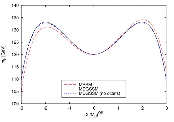
Figure 2: Mass of the SM-like Higgs boson as a function of $(X_{t}/M_{S})^{\rm OS}$, for $\tan\beta=10$, $M_{S}=1.5$ TeV and $m_{\tilde{g}}=m_{O}=2$ TeV. The dashed curve represents the MSSM result, whereas the solid (dotted) curve represents the MDGSSM result with (without) the octet-scalar contributions.

Figure 3: Different determinations of the SM-like Higgs boson mass in the MDGSSM as a function of $(X_{t}/M_{S})^{\rm OS}$, for the same choices of parameters as in figure 2. The solid curve represents the original OS calculation; the dotted curve represents the ${\overline{\rm DR}}$ calculation; the dashed and dot-dashed curves were obtained using $\hat{\alpha}_{s}(m_{t})$ and $\overline{\alpha}_{s}(m_{t})$, respectively, in the OS calculation instead of $\hat{\alpha}_{s}(M_{S})$.

A discussion of the theoretical uncertainty of our calculation is now in order. In our numerical examples we are not implementing the full one-loop corrections to the Higgs boson masses, nor the two-loop corrections beyond ${\cal O}(\alpha_{t}\alpha_{s})$ that are available in SARAH, in order to focus purely on the ${\cal O}(\alpha_{t}\alpha_{s})$ corrections. Therefore the only sources of uncertainty that we can meaningfully estimate are the uncomputed effects of ${\cal O}(\alpha_{t}\alpha_{s}^{2})$, i.e. those arising from genuine three-loop diagrams with four strong-interaction vertices and from SUSY-QCD renormalisation effects of the parameters entering the one- and two-loop corrections. A common procedure for estimating those effects consists in comparing the results of the ${\cal O}(\alpha_{t}\alpha_{s})$ calculation of $m_{h}$ in the OS scheme with the results obtained by $i)$ converting the OS input parameters – i.e., the top mass and the stop masses and mixing – to the ${\overline{\rm DR}}$ scheme by means of ${\cal O}(\alpha_{s})$ shifts, and $ii)$ computing $m_{h}$ using these ${\overline{\rm DR}}$ parameters in both the one-loop and two-loop corrections, with the appropriate ${\overline{\rm DR}}$ formulae for the ${\cal O}(\alpha_{t}\alpha_{s})$ corrections. The two sources of ${\cal O}(\alpha_{t}\alpha_{s}^{2})$ discrepancies in such a comparison are the omission of terms quadratic in $\delta x_{k}$ in the expansion of the one-loop part of the corrections, eq. (3.58), and the different definition of the top and stop parameters entering the two-loop part of the corrections. In figure 3 we illustrate the renormalisation-scheme dependence of the ${\cal O}(\alpha_{t}\alpha_{s})$ determination of $m_{h}$, in the same MDGSSM scenario as in figure 2. The solid (black) curve represents the results of the original OS calculation, whereas the dotted (blue) curve represents the results of the ${\overline{\rm DR}}$ calculation described above (note that both curves are plotted as functions of the ratio of OS parameters $X_{t}/M_{S}$). The comparison between the solid and dotted curves would suggest a rather small impact of the uncomputed ${\cal O}(\alpha_{t}\alpha_{s}^{2})$ corrections, of the order of one GeV or even less (at least for the considered scenario).

Besides the top mass and the stop masses and mixing, there are a few more parameters entering the ${\cal O}(\alpha_{t}\alpha_{s})$ corrections to the Higgs boson masses whose ${\cal O}(\alpha_{s})$ definition amounts to a three-loop ${\cal O}(\alpha_{t}\alpha_{s}^{2})$ effect, namely the gluino and octet-scalar masses and the strong gauge coupling itself. Concerning the masses, in an OS calculation it seems natural to interpret them as pole ones. For $\alpha_{s}$, on the other hand, there is no obvious “on-shell” definition available, and different choices of scheme, scale and even underlying theory – while all formally equivalent at ${\cal O}(\alpha_{t}\alpha_{s})$ for the Higgs-mass calculation – can lead to significant variations in the numerical results. As mentioned earlier, the solid curve in figure 3 was obtained with top/stop parameters in the OS scheme, but with $\alpha_{s}$ defined as the ${\overline{\rm DR}}$-renormalised coupling of the MDGSSM at the stop-mass scale, i.e. $\hat{\alpha}_{s}(M_{S})$. However, since both stop squarks and top quarks enter the relevant two-loop diagrams, it would not seem unreasonable to evaluate the strong gauge coupling at the top-mass scale either. The dashed (red) and dot-dashed (green) curves in figure 3 represent the predictions for $m_{h}$ obtained with top/stop parameters still in the OS scheme, but with $\alpha_{s}$ defined as the ${\overline{\rm DR}}$-renormalised coupling of the MDGSSM at the top-mass scale, $\hat{\alpha}_{s}(m_{t})$, and as the $\overline{\rm MS}$-renormalised coupling of the SM at the same scale, $\overline{\alpha}_{s}(m_{t})$, respectively. The comparison of these two curves with the solid curve shows that a variation in the definition of the coupling $\alpha_{s}$ entering the two-loop corrections provides a less-optimistic estimate of the uncertainty associated to the ${\cal O}(\alpha_{t}\alpha_{s}^{2})$ corrections compared with the scheme variation of the top/stop parameters. In particular, for the considered scenario the use of $\overline{\alpha}_{s}(m_{t})$ would induce a negative variation with respect to the results obtained with $\hat{\alpha}_{s}(M_{S})$ of about $4$ GeV for $X_{t}\approx 0$ and about $7$ GeV for $|X_{t}/M_{S}|\approx 2$. In contrast, the use of $\hat{\alpha}_{s}(m_{t})$ would induce a positive variation of about $1$ GeV for $X_{t}\approx 0$ and about $2$ GeV for $|X_{t}/M_{S}|\approx 2$, i.e. more modest than the previous one but still larger than the one induced by a scheme change in the top/stop parameters. While remaining agnostic about the true size (and sign) of the three-loop ${\cal O}(\alpha_{t}\alpha_{s}^{2})$ corrections, we take this as a cautionary tale against putting too much stock in any single estimate of the theoretical uncertainty of a fixed-order calculation of $m_{h}$ in scenarios with TeV-scale superparticles.

4.2 An example in the MRSSM

In our second numerical example we consider the MRSSM, and illustrate the dependence of the SM-like Higgs boson mass on the gluino mass. In ref. [68] it was pointed out that, for multi-TeV values of $m_{\tilde{g}}$, the contribution of two-loop diagrams involving octet scalars can increase the prediction for $m_{h}$ by more than $10$ GeV. We will show that such large effects are related to the non-decoupling behaviour of the ${\overline{\rm DR}}$ calculation of $m_{h}$ that we discussed in section 3.7.2, and that the octet-scalar contributions are much more modest in an OS calculation.

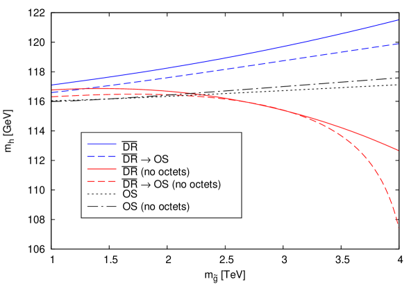
Figure 4: Mass of the SM-like Higgs boson as a function of $m_{\tilde{g}}$ in the MRSSM, for $\tan\beta=10$, $M_{S}=1$ TeV and $m_{O}=2$ TeV. The meaning of the different curves is explained in the text.

The upper (blue) and lower (red) solid curves in figure 4 represent the SM-like Higgs boson mass obtained from the ${\overline{\rm DR}}$ calculation as a function of $m_{\tilde{g}}$, with and without the octet-scalar contributions, respectively. We set $m_{O}=2$ TeV and $M_{S}=1$ TeV. The latter is interpreted as a ${\overline{\rm DR}}$-renormalised soft SUSY-breaking parameter evaluated at a scale equal to $M_{S}$ itself, which means that each point in the solid curves corresponds to a different value of the physical stop masses. Both curves show a marked dependence on $m_{\tilde{g}}$, and the comparison between them shows that, for the highest value of $m_{\tilde{g}}$ considered in the plot, the effect on $m_{h}$ of the two-loop octet-scalar contributions does indeed grow to about $9$ GeV. However, as can be seen in the explicit formulae for the two-loop corrections in the ${\overline{\rm DR}}$ scheme of eqs. (3.70) and (3.74), this marked dependence of both the gluino and octet-scalar contributions on $m_{\tilde{g}}$ is induced by terms enhanced by the ratio $m_{\tilde{g}}^{2}/M_{S}^{2}$. When that ratio becomes large, which in Dirac-gaugino models can occur naturally, the size of the two-loop ${\cal O}(\alpha_{t}\alpha_{s})$ corrections to $m_{h}$ can grow up to a point where the accuracy of the perturbative expansion is called into question. To visualise this aspect, we perform a change of renormalisation scheme for the top and stop masses that mirrors the one represented by the dotted curve in figure 3. The upper (blue) and lower (red) dashed curves in figure 4 represent the values of $m_{h}$ obtained with and without octet-scalar contributions, respectively, after converting the ${\overline{\rm DR}}$ stop masses into the physical ones and using the latter, together with the physical top mass, in both the one-loop and two-loop corrections, with the appropriate OS formulae for the ${\cal O}(\alpha_{t}\alpha_{s})$ corrections. For our choice of the ${\overline{\rm DR}}$ input parameter $M_{S}(M_{S})=1$ TeV, we find that the physical stop masses range between $1072$ GeV and $1392$ GeV for the values of $m_{\tilde{g}}$ shown in the plot. If the octet-scalar contributions to the ${\cal O}(\alpha_{s})$ stop self-energies are omitted, the stop masses range instead between $1049$ GeV and $346$ GeV, i.e. they become smaller for increasing $m_{\tilde{g}}$ (indeed, in this case $m_{\tilde{g}}$ cannot be pushed to values much larger than those shown in the plot without rendering the stop masses tachyonic). The comparison between the solid and dashed curves shows that the scheme dependence of the ${\cal O}(\alpha_{t}\alpha_{s})$ calculation of $m_{h}$ becomes increasingly worse at large values of $m_{\tilde{g}}$, especially in the lower curves where the octet-scalar contributions are omitted. Finally, the (black) dotted and dot-dashed curves in figure 4 represent the predictions for $m_{h}$ obtained directly from the OS calculation with and without octet-scalar contributions, respectively. In this case the input $M_{S}=1$ TeV is interpreted as an OS-renormalised parameter, meaning that the physical stop masses correspond to $(M_{S}^{2}+m_{t}^{2})^{1/2}\approx 1015$ GeV for all points in the curves. We stress that direct comparisons between these two curves and the solid (and dashed) ones would not be appropriate, because they refer to different points of the MRSSM parameter space. However, the dotted and dot-dashed curves show that, when the physical stop masses are taken as input, the prediction for $m_{h}$ in the MRSSM depends only mildly on the value of $m_{\tilde{g}}$, and the effect of the octet-scalar contributions is below one GeV. This is explained by the fact that, as discussed in section 3.7.2, in the OS scheme there are no terms enhanced by $m_{\tilde{g}}^{2}/M_{S}^{2}$ in either the gluino or the octet-scalar contributions to the ${\cal O}(\alpha_{t}\alpha_{s})$ corrections.

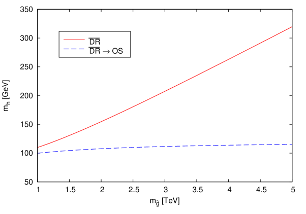
Figure 5: Mass of the SM-like Higgs boson as a function of $m_{\tilde{g}}$ in the supersoft limit of the MRSSM, for $\tan\beta=10$. The solid curve represents the results of the ${\overline{\rm DR}}$ calculation, in which the two-loop ${\cal O}(\alpha_{t}\alpha_{s})$ corrections become unphysically large. The dashed curve was obtained by converting the top and stop masses to the OS scheme and using the corresponding formulae for the ${\cal O}(\alpha_{t}\alpha_{s})$ corrections.

Before concluding, we note that there are extreme situations in which a ${\overline{\rm DR}}$ calculation of $m_{h}$ is not workable at all, and a conversion to the OS scheme such as the one represented by the dashed lines in figure 4 is necessary. In the so-called supersoft scenario, all soft SUSY-breaking masses vanish, and sizeable sfermion masses – proportional to the Dirac-gaugino masses – are induced only by radiative corrections. Such a scenario can be realised e.g. in the MRSSM by setting $m_{O}=0$ and $M_{S}=0$, where the latter is interpreted as a ${\overline{\rm DR}}$-renormalised parameter. At the scale where this condition is imposed, the ${\overline{\rm DR}}$ stop masses coincide with the top mass, with the result that, in the ${\overline{\rm DR}}$ calculation, the one-loop correction in the first term of eq. (3.69) vanishes, while the two-loop corrections in eqs. (3.70) and (3.74) contain terms enhanced by $m_{\tilde{g}}^{2}/m_{t}^{2}$ (concerning the octet-scalar contributions, we recall that $m_{O_{1}}=2\,m_{\tilde{g}}$ in this scenario). Since the Dirac-gluino mass needs to be in the multi-TeV range to generate realistic values for the physical stop masses, the non-decoupling terms in the two-loop corrections can become unphysically large. This is illustrated by the solid (red) curve in figure 5, which represents the SM-like Higgs boson mass obtained with the ${\overline{\rm DR}}$ calculation as a function of the gluino mass (here we fix the renormalisation scale as $Q=m_{t}$ and use $\overline{\alpha}_{s}(m_{t})$ in the two-loop corrections). It appears that the ${\overline{\rm DR}}$ prediction for $m_{h}$ becomes essentially proportional to $m_{\tilde{g}}$, and quickly grows to nonsensical values as the latter increases. In contrast, the dashed (blue) curve is obtained with the same procedure as the dashed curves in figure 4, i.e. by computing the physical stop masses at ${\cal O}(\alpha_{s})$ as a function of $m_{\tilde{g}}$ and using them in conjunction with the appropriate OS formulae for the ${\cal O}(\alpha_{t}\alpha_{s})$ corrections to $m_{h}$. In our example the stop masses range between $302$ GeV and $1272$ GeV, while the SM-like Higgs boson mass shows only a mild dependence on $m_{\tilde{g}}$ and remains confined to values well below the observed one.

5 Conclusions

Supersymmetric models with Dirac gaugino masses have attracted considerable attention in the past few years, because they are subject to looser experimental constraints and require less fine-tuning than the MSSM. Besides the extended gaugino sector, such models feature additional colourless scalars which mix with the usual Higgs doublets of the MSSM, as well as additional coloured scalars in the octet representation of $SU(3)$ which contribute to the Higgs boson masses at the two-loop level. In this paper we presented a computation of the dominant two-loop corrections to the Higgs boson masses in Dirac-gaugino models, relying on effective-potential techniques that had previously been applied to the MSSM [36] and to the NMSSM [49]. We obtained analytic formulae for the ${\cal O}(\alpha_{t}\alpha_{s})$ corrections to the scalar and pseudoscalar Higgs mass matrices valid for arbitrary choices of parameters in the squark and gaugino sectors, both in the ${\overline{\rm DR}}$ and in the OS renormalisation schemes, which we make available upon request as a fortran code. We also presented compact approximate formulae for the dominant corrections to the mass of the SM-like Higgs boson, valid under a number of simplifying assumptions for the SUSY parameters. Finally, we studied the numerical impact of the newly-computed corrections on the predictions for the SM-like Higgs boson mass in some representative scenarios. In particular, we elucidated the differences between the predictions for $m_{h}$ in the MSSM and those in its Dirac-gaugino extensions; we discussed the theoretical uncertainty of our predictions stemming from uncomputed higher-order corrections; we stressed that a judicious choice of renormalisation scheme is required to obtain reliable predictions in scenarios where the gluinos are much heavier than the squarks, which can occur naturally in Dirac-gaugino models. If our community’s hopes are fulfilled and the run II of the LHC brings on a wealth of new discoveries, our results will contribute to their accurate interpretation in the framework of a well-motivated SUSY extension of the SM.

Appendix A Derivatives of the two-loop effective potential

We present here the derivatives of the two-loop effective potential used to calculate the Higgs masses in section 3. We recall that the effective potential and its derivatives are expressed in units of $\alpha_{s}\,C_{F}N_{c}/(4\pi)^{3}$. The derivatives of the first term in eq. (3.19) can be trivially obtained by multiplying the formulae in appendix C of ref. [49] by $R_{1i}^{2}$ and summing over the two gluino masses $m_{\tilde{g}_{i}}\,$, hence we do not repeat them here. The only exception is the single derivative of $\Delta V^{\,\alpha_{s}}_{{\rm{\scriptscriptstyle MSSM}}}$ with respect to $m_{t}^{2}$, which was not needed in ref. [49]. Adapted to the Dirac-gaugino case, it reads

$$\frac{~{}\,\partial\Delta V^{\,\alpha_{s}}}{\partial m_{t}^{2}}~{}=~{}\sum_{i=1}^{2}\,R_{1i}^{2}\,\frac{~{}\partial\Delta V_{\tilde{g}_{i}}}{\partial m_{t}^{2}}~{},$$ (A.1)

with

$$\frac{\partial\Delta V_{\tilde{g}_{i}}}{\partial m_{t}^{2}}\!\! = 2\,m_{t}^{2}\left(3-4\,\ln\frac{m_{t}^{2}}{Q^{2}}+3\,\ln^{2}\frac{m_{t}^{2}}{Q^{2}}\right)~{}+~{}2\,\left[m_{t}^{2}\,\ln\frac{m_{\tilde{g}_{i}}^{2}}{m_{t}^{2}}+m_{\tilde{t}_{1}}^{2}\biggr{(}2-\ln\frac{m_{t}^{2}}{Q^{2}}-\ln\frac{m_{\tilde{g}_{i}}^{2}}{Q^{2}}\biggr{)}\right]\,\ln\frac{m_{\tilde{t}_{1}}^{2}}{Q^{2}}$$ (A.2)

$$+ \!\!\!\left[2\,(m_{\tilde{t}_{1}}^{2}-m_{t}^{2})-\frac{m_{\tilde{g}_{i}}\,m_{\tilde{t}_{1}}^{2}s_{2\theta_{t}}}{m_{t}}\right]\ln\frac{m_{t}^{2}}{Q^{2}}\ln\frac{m_{\tilde{g}_{i}}^{2}}{Q^{2}}-2\,m_{\tilde{g}_{i}}^{2}\biggr{(}3-2\,\ln\frac{m_{\tilde{g}_{i}}^{2}}{Q^{2}}\biggr{)}-m_{\tilde{t}_{1}}^{2}\!\left(4-\frac{5\,m_{\tilde{g}_{i}}s_{2\theta_{t}}}{m_{t}}\right)$$

$$- \frac{m_{\tilde{g}_{i}}\,s_{2\theta_{t}}}{m_{t}}\,\left[\left(3\,m_{t}^{2}-m_{\tilde{g}_{i}}^{2}\right)\,\ln\frac{m_{\tilde{g}_{i}}^{2}}{m_{t}^{2}}\,+\,m_{\tilde{t}_{1}}^{2}\biggr{(}4-\ln\frac{m_{t}^{2}}{Q^{2}}-\ln\frac{m_{\tilde{g}_{i}}^{2}}{Q^{2}}\biggr{)}\right]\,\ln\frac{m_{\tilde{t}_{1}}^{2}}{Q^{2}}$$

$$+ \!2\left[\frac{m_{\tilde{g}_{i}}^{2}}{m_{t}^{2}}\,(m_{\tilde{g}_{i}}^{2}-m_{t}^{2}-m_{\tilde{t}_{1}}^{2})-\frac{\Delta_{\tilde{g}_{i}}}{m_{t}^{2}}\,+\,\frac{m_{\tilde{g}_{i}}\,s_{2\theta_{t}}}{m_{t}}\,\biggr{(}m_{t}^{2}-m_{\tilde{g}_{i}}^{2}-m_{\tilde{t}_{1}}^{2}+\frac{\Delta_{\tilde{g}_{i}}}{2\,m_{t}^{2}}\biggr{)}\right]\,\Phi(m_{\tilde{t}_{1}}^{2},m_{\tilde{g}_{i}}^{2},m_{t}^{2})$$

$$+ ~{}\biggr{[}m_{\tilde{t}_{1}}^{2}\,\rightarrow\,m_{\tilde{t}_{2}}^{2}~{},~{}~{}~{}~{}s_{2\theta_{t}}\,\rightarrow\,-s_{2\theta_{t}}\biggr{]}~{},$$

where $Q$ is the renormalisation scale, the function $\Phi(x,y,z)$ is defined in appendix D of ref. [49], and we used the shortcut

$$\Delta_{\tilde{g}_{i}}~{}\equiv~{}(m_{\tilde{g}_{i}}^{2}-m_{t}^{2}-m_{\tilde{t}_{1}}^{2})^{2}-4\,m_{t}^{2}m_{\tilde{t}_{1}}^{2}~{}.$$ (A.3)

The derivatives of the octet-scalar contribution $\Delta V_{O_{i}}$, computed at the minimum of the potential, are

$$\frac{\partial\Delta V_{O_{i}}}{\partial c_{2\bar{\theta}_{t}}^{2}} = -2\bigg{[}I(m_{\tilde{t}_{1}}^{2},m_{\tilde{t}_{1}}^{2},m_{O_{i}}^{2})+I(m_{\tilde{t}_{2}}^{2},m_{\tilde{t}_{2}}^{2},m_{O_{i}}^{2})-2I(m_{\tilde{t}_{1}}^{2},m_{\tilde{t}_{2}}^{2},m_{O_{i}}^{2})\bigg{]}~{},$$ (A.4)

$$\frac{\partial\Delta V_{O_{i}}}{\partial m_{\tilde{t}_{1}}^{2}} = 2\,\Big{(}\ln\frac{m_{\tilde{t}_{1}}^{2}}{Q^{2}}-1\Big{)}^{2}+2\,s_{2\theta_{t}}^{2}\ln\frac{m_{O_{i}}^{2}}{m_{\tilde{t}_{1}}^{2}}\ln\frac{m_{\tilde{t}_{1}}^{2}}{m_{\tilde{t}_{2}}^{2}}$$ (A.5)

$$-2\,\bigg{[}c_{2\theta_{t}}^{2}\Phi(m_{\tilde{t}_{1}}^{2},m_{\tilde{t}_{1}}^{2},m_{O_{i}}^{2})+s_{2\theta_{t}}^{2}\frac{m_{O_{i}}^{2}-m_{\tilde{t}_{1}}^{2}+m_{\tilde{t}_{2}}^{2}}{m_{O_{i}}^{2}}\Phi(m_{\tilde{t}_{1}}^{2},m_{\tilde{t}_{2}}^{2},m_{O_{i}}^{2})\bigg{]}~{},$$

$$\frac{\partial^{2}\Delta V_{O_{i}}}{(\partial m_{\tilde{t}_{1}}^{2})^{2}} = -\frac{4\,s_{2\theta_{t}}^{2}}{m_{\tilde{t}_{1}}^{2}}+\frac{4\,c_{2\theta_{t}}^{2}}{m_{O_{i}}^{2}-4m_{\tilde{t}_{1}}^{2}}\bigg{[}\frac{m_{O_{i}}^{2}}{m_{\tilde{t}_{1}}^{2}}\Big{(}\ln\frac{m_{O_{i}}^{2}}{Q^{2}}-1\Big{)}-4\Big{(}\ln\frac{m_{\tilde{t}_{1}}^{2}}{Q^{2}}-1\Big{)}-\Phi(m_{\tilde{t}_{1}}^{2},m_{\tilde{t}_{1}}^{2},m_{O_{i}}^{2})\bigg{]}$$ (A.6)

$$+\frac{4\,s_{2\theta_{t}}^{2}}{\Delta_{O_{i}}}\,\bigg{[}\frac{m_{O_{i}}^{2}}{m_{\tilde{t}_{1}}^{2}}(m_{O_{i}}^{2}-m_{\tilde{t}_{1}}^{2}-m_{\tilde{t}_{2}}^{2})\ln\frac{m_{O_{i}}^{2}}{Q^{2}}-(m_{O_{i}}^{2}-m_{\tilde{t}_{1}}^{2}+m_{\tilde{t}_{2}}^{2})\ln\frac{m_{\tilde{t}_{1}}^{2}}{Q^{2}}$$

$$~{}~{}~{}~{}~{}~{}~{}~{}~{}~{}~{}~{}-\frac{m_{\tilde{t}_{2}}^{2}}{m_{\tilde{t}_{1}}^{2}}(m_{O_{i}}^{2}+m_{\tilde{t}_{1}}^{2}-m_{\tilde{t}_{2}}^{2})\ln\frac{m_{\tilde{t}_{2}}^{2}}{Q^{2}}-2\,m_{\tilde{t}_{2}}^{2}\,\Phi(m_{\tilde{t}_{1}}^{2},m_{\tilde{t}_{2}}^{2},m_{O_{i}}^{2})\bigg{]}~{},$$

$$\frac{\partial^{2}\Delta V_{O_{i}}}{\partial m_{\tilde{t}_{1}}^{2}\partial c_{2\bar{\theta}_{t}}^{2}} = -2\bigg{[}\ln\frac{m_{O_{i}}^{2}}{m_{\tilde{t}_{1}}^{2}}\ln\frac{m_{\tilde{t}_{1}}^{2}}{m_{\tilde{t}_{2}}^{2}}+\Phi(m_{\tilde{t}_{1}}^{2},m_{\tilde{t}_{1}}^{2},m_{O_{i}}^{2})-\frac{m_{O_{i}}^{2}-m_{\tilde{t}_{1}}^{2}+m_{\tilde{t}_{2}}^{2}}{m_{O_{i}}^{2}}\,\Phi(m_{\tilde{t}_{1}}^{2},m_{\tilde{t}_{2}}^{2},m_{O_{i}}^{2})\bigg{]}~{},$$ (A.7)

$$\frac{\partial^{2}\Delta V_{O_{i}}}{\partial m_{\tilde{t}_{1}}^{2}\partial m_{\tilde{t}_{2}}^{2}} = \frac{4\,s_{2\theta_{t}}^{2}}{\Delta_{O_{i}}}\,\bigg{[}m_{O_{i}}^{2}\ln\frac{m_{O_{i}}^{4}}{m_{\tilde{t}_{1}}^{2}m_{\tilde{t}_{2}}^{2}}-(m_{\tilde{t}_{1}}^{2}-m_{\tilde{t}_{2}}^{2})\ln\frac{m_{\tilde{t}_{1}}^{2}}{m_{\tilde{t}_{2}}^{2}}-(m_{O_{i}}^{2}-m_{\tilde{t}_{1}}^{2}-m_{\tilde{t}_{2}}^{2})\Phi(m_{\tilde{t}_{1}}^{2},m_{\tilde{t}_{2}}^{2},m_{O_{i}}^{2})\bigg{]}~{},$$

where we used the shortcut

$$\Delta_{O_{i}}~{}\equiv~{}(m_{O_{i}}^{2}-m_{\tilde{t}_{1}}^{2}-m_{\tilde{t}_{2}}^{2})^{2}-4\,m_{\tilde{t}_{1}}^{2}m_{\tilde{t}_{2}}^{2}~{}.$$ (A.9)

The derivatives of $\Delta V_{O_{i}}$ that involve $m_{\tilde{t}_{2}}^{2}$ can be trivially obtained from the ones in eqs. (A.5)–(A.7) by means of the replacement $m_{\tilde{t}_{1}}^{2}\!\leftrightarrow m_{\tilde{t}_{2}}^{2}$, while the derivatives with respect to all other combinations of field-dependent parameters vanish.

References

• [1] P. Fayet, Massive Gluinos. Phys. Lett. B78 (1978) 417–420.
• [2] J. Polchinski and L. Susskind, Breaking of Supersymmetry at Intermediate-Energy. Phys. Rev. D26 (1982) 3661.
• [3] L. J. Hall and L. Randall, U(1)-R symmetric supersymmetry. Nucl. Phys. B352 (1991) 289–308.
• [4] P. J. Fox, A. E. Nelson, and N. Weiner, Dirac gaugino masses and supersoft supersymmetry breaking. JHEP 08 (2002) 035, arXiv:hep-ph/0206096 [hep-ph].
• [5] A. E. Nelson, N. Rius, V. Sanz, and M. Unsal, The Minimal supersymmetric model without a mu term. JHEP 08 (2002) 039, arXiv:hep-ph/0206102 [hep-ph].
• [6] I. Antoniadis, K. Benakli, A. Delgado, and M. Quiros, A New gauge mediation theory. Adv. Stud. Theor. Phys. 2 (2008) 645–672, arXiv:hep-ph/0610265 [hep-ph].
• [7] M. Heikinheimo, M. Kellerstein, and V. Sanz, How Many Supersymmetries? JHEP 04 (2012) 043, arXiv:1111.4322 [hep-ph].
• [8] G. D. Kribs and A. Martin, Supersoft Supersymmetry is Super-Safe. Phys. Rev. D85 (2012) 115014, arXiv:1203.4821 [hep-ph].
• [9] G. D. Kribs and A. Martin, Dirac Gauginos in Supersymmetry – Suppressed Jets + MET Signals: A Snowmass Whitepaper. arXiv:1308.3468 [hep-ph].
• [10] G. D. Kribs, E. Poppitz, and N. Weiner, Flavor in supersymmetry with an extended R-symmetry. Phys. Rev. D78 (2008) 055010, arXiv:0712.2039 [hep-ph].
• [11] R. Fok and G. D. Kribs, $\mu$ to e in R-symmetric Supersymmetry. Phys. Rev. D82 (2010) 035010, arXiv:1004.0556 [hep-ph].
• [12] E. Dudas, M. Goodsell, L. Heurtier, and P. Tziveloglou, Flavour models with Dirac and fake gluinos. Nucl. Phys. B884 (2014) 632–671, arXiv:1312.2011 [hep-ph].
• [13] G. Belanger, K. Benakli, M. Goodsell, C. Moura, and A. Pukhov, Dark Matter with Dirac and Majorana Gaugino Masses. JCAP 0908 (2009) 027, arXiv:0905.1043 [hep-ph].
• [14] K. Benakli, M. D. Goodsell, and A.-K. Maier, Generating mu and Bmu in models with Dirac Gauginos. Nucl. Phys. B851 (2011) 445–461, arXiv:1104.2695 [hep-ph].
• [15] K. Benakli, M. Goodsell, F. Staub, and W. Porod, Constrained minimal Dirac gaugino supersymmetric standard model. Phys. Rev. D90 (2014) no. 4, 045017, arXiv:1403.5122 [hep-ph].
• [16] M. D. Goodsell, M. E. Krauss, T. Müller, W. Porod, and F. Staub, Dark matter scenarios in a constrained model with Dirac gauginos. JHEP 10 (2015) 132, arXiv:1507.01010 [hep-ph].
• [17] K. Benakli, L. Darmé, M. D. Goodsell, and J. Harz, The Di-Photon Excess in a Perturbative SUSY Model. arXiv:1605.05313 [hep-ph].
• [18] A. E. Nelson and N. Seiberg, R symmetry breaking versus supersymmetry breaking. Nucl. Phys. B416 (1994) 46–62, arXiv:hep-ph/9309299 [hep-ph].
• [19] S. D. L. Amigo, A. E. Blechman, P. J. Fox, and E. Poppitz, R-symmetric gauge mediation. JHEP 01 (2009) 018, arXiv:0809.1112 [hep-ph].
• [20] K. Benakli and M. D. Goodsell, Dirac Gauginos in General Gauge Mediation. Nucl. Phys. B816 (2009) 185–203, arXiv:0811.4409 [hep-ph].
• [21] K. Benakli and M. D. Goodsell, Dirac Gauginos, Gauge Mediation and Unification. Nucl. Phys. B840 (2010) 1–28, arXiv:1003.4957 [hep-ph].
• [22] L. M. Carpenter, Dirac Gauginos, Negative Supertraces and Gauge Mediation. JHEP 09 (2012) 102, arXiv:1007.0017 [hep-th].
• [23] S. Abel and M. Goodsell, Easy Dirac Gauginos. JHEP 06 (2011) 064, arXiv:1102.0014 [hep-th].
• [24] C. Csaki, J. Goodman, R. Pavesi, and Y. Shirman, The $m_{D}-b_{M}$ problem of Dirac gauginos and its solutions. Phys. Rev. D89 (2014) no. 5, 055005, arXiv:1310.4504 [hep-ph].
• [25] K. Benakli, M. D. Goodsell, and F. Staub, Dirac Gauginos and the 125 GeV Higgs. JHEP 06 (2013) 073, arXiv:1211.0552 [hep-ph].
• [26] C. Frugiuele and T. Gregoire, Making the Sneutrino a Higgs with a $U(1)_{R}$ Lepton Number. Phys. Rev. D85 (2012) 015016, arXiv:1107.4634 [hep-ph].
• [27] E. Bertuzzo, C. Frugiuele, T. Gregoire, and E. Ponton, Dirac gauginos, R symmetry and the 125 GeV Higgs. JHEP 04 (2015) 089, arXiv:1402.5432 [hep-ph].
• [28] R. Davies, J. March-Russell, and M. McCullough, A Supersymmetric One Higgs Doublet Model. JHEP 04 (2011) 108, arXiv:1103.1647 [hep-ph].
• [29] R. Hempfling and A. H. Hoang, Two loop radiative corrections to the upper limit of the lightest Higgs boson mass in the minimal supersymmetric model. Phys. Lett. B331 (1994) 99–106, arXiv:hep-ph/9401219 [hep-ph].
• [30] S. Heinemeyer, W. Hollik, and G. Weiglein, QCD corrections to the masses of the neutral CP - even Higgs bosons in the MSSM. Phys. Rev. D58 (1998) 091701, arXiv:hep-ph/9803277 [hep-ph].
• [31] S. Heinemeyer, W. Hollik, and G. Weiglein, Precise prediction for the mass of the lightest Higgs boson in the MSSM. Phys. Lett. B440 (1998) 296–304, arXiv:hep-ph/9807423 [hep-ph].
• [32] R.-J. Zhang, Two loop effective potential calculation of the lightest CP even Higgs boson mass in the MSSM. Phys. Lett. B447 (1999) 89–97, arXiv:hep-ph/9808299 [hep-ph].
• [33] S. Heinemeyer, W. Hollik, and G. Weiglein, The Masses of the neutral CP - even Higgs bosons in the MSSM: Accurate analysis at the two loop level. Eur. Phys. J. C9 (1999) 343–366, arXiv:hep-ph/9812472 [hep-ph].
• [34] J. R. Espinosa and R.-J. Zhang, MSSM lightest CP even Higgs boson mass to O(alpha(s) alpha(t)): The Effective potential approach. JHEP 03 (2000) 026, arXiv:hep-ph/9912236 [hep-ph].
• [35] J. R. Espinosa and R.-J. Zhang, Complete two loop dominant corrections to the mass of the lightest CP even Higgs boson in the minimal supersymmetric standard model. Nucl. Phys. B586 (2000) 3–38, arXiv:hep-ph/0003246 [hep-ph].
• [36] G. Degrassi, P. Slavich, and F. Zwirner, On the neutral Higgs boson masses in the MSSM for arbitrary stop mixing. Nucl. Phys. B611 (2001) 403–422, arXiv:hep-ph/0105096 [hep-ph].
• [37] A. Brignole, G. Degrassi, P. Slavich, and F. Zwirner, On the O(alpha(t)**2) two loop corrections to the neutral Higgs boson masses in the MSSM. Nucl. Phys. B631 (2002) 195–218, arXiv:hep-ph/0112177 [hep-ph].
• [38] A. Brignole, G. Degrassi, P. Slavich, and F. Zwirner, On the two loop sbottom corrections to the neutral Higgs boson masses in the MSSM. Nucl. Phys. B643 (2002) 79–92, arXiv:hep-ph/0206101 [hep-ph].
• [39] S. P. Martin, Two loop effective potential for the minimal supersymmetric standard model. Phys. Rev. D66 (2002) 096001, arXiv:hep-ph/0206136 [hep-ph].
• [40] S. P. Martin, Complete two loop effective potential approximation to the lightest Higgs scalar boson mass in supersymmetry. Phys. Rev. D67 (2003) 095012, arXiv:hep-ph/0211366 [hep-ph].
• [41] A. Dedes, G. Degrassi, and P. Slavich, On the two loop Yukawa corrections to the MSSM Higgs boson masses at large tan beta. Nucl. Phys. B672 (2003) 144–162, arXiv:hep-ph/0305127 [hep-ph].
• [42] S. Heinemeyer, W. Hollik, H. Rzehak, and G. Weiglein, High-precision predictions for the MSSM Higgs sector at O(alpha(b) alpha(s)). Eur. Phys. J. C39 (2005) 465–481, arXiv:hep-ph/0411114 [hep-ph].
• [43] S. P. Martin, Strong and Yukawa two-loop contributions to Higgs scalar boson self-energies and pole masses in supersymmetry. Phys. Rev. D71 (2005) 016012, arXiv:hep-ph/0405022 [hep-ph].
• [44] S. Borowka, T. Hahn, S. Heinemeyer, G. Heinrich, and W. Hollik, Momentum-dependent two-loop QCD corrections to the neutral Higgs-boson masses in the MSSM. Eur. Phys. J. C74 (2014) no. 8, 2994, arXiv:1404.7074 [hep-ph].
• [45] G. Degrassi, S. Di Vita, and P. Slavich, Two-loop QCD corrections to the MSSM Higgs masses beyond the effective-potential approximation. Eur. Phys. J. C75 (2015) no. 2, 61, arXiv:1410.3432 [hep-ph].
• [46] S. P. Martin, Three-loop corrections to the lightest Higgs scalar boson mass in supersymmetry. Phys. Rev. D75 (2007) 055005, arXiv:hep-ph/0701051 [hep-ph].
• [47] R. V. Harlander, P. Kant, L. Mihaila, and M. Steinhauser, Higgs boson mass in supersymmetry to three loops. Phys. Rev. Lett. 100 (2008) 191602, arXiv:0803.0672 [hep-ph]. [Phys. Rev. Lett.101,039901(2008)].
• [48] P. Kant, R. V. Harlander, L. Mihaila, and M. Steinhauser, Light MSSM Higgs boson mass to three-loop accuracy. JHEP 08 (2010) 104, arXiv:1005.5709 [hep-ph].
• [49] G. Degrassi and P. Slavich, On the radiative corrections to the neutral Higgs boson masses in the NMSSM. Nucl. Phys. B825 (2010) 119–150, arXiv:0907.4682 [hep-ph].
• [50] M. Mühlleitner, D. T. Nhung, H. Rzehak, and K. Walz, Two-loop contributions of the order $\mathcal{O}\left({\alpha}_{t}{\alpha}_{s}\right)$ to the masses of the Higgs bosons in the CP-violating NMSSM. JHEP 05 (2015) 128, arXiv:1412.0918 [hep-ph].
• [51] F. Staub, SARAH. arXiv:0806.0538 [hep-ph].
• [52] F. Staub, From Superpotential to Model Files for FeynArts and CalcHep/CompHep. Comput. Phys. Commun. 181 (2010) 1077–1086, arXiv:0909.2863 [hep-ph].
• [53] F. Staub, Automatic Calculation of supersymmetric Renormalization Group Equations and Self Energies. Comput. Phys. Commun. 182 (2011) 808–833, arXiv:1002.0840 [hep-ph].
• [54] F. Staub, SARAH 3.2: Dirac Gauginos, UFO output, and more. Comput. Phys. Commun. 184 (2013) 1792–1809, arXiv:1207.0906 [hep-ph].
• [55] F. Staub, SARAH 4 : A tool for (not only SUSY) model builders. Comput. Phys. Commun. 185 (2014) 1773–1790, arXiv:1309.7223 [hep-ph].
• [56] F. Staub, Exploring new models in all detail with SARAH. Adv. High Energy Phys. 2015 (2015) 840780, arXiv:1503.04200 [hep-ph].
• [57] M. D. Goodsell, K. Nickel, and F. Staub, Two-Loop Higgs mass calculations in supersymmetric models beyond the MSSM with SARAH and SPheno. Eur. Phys. J. C75 (2015) no. 1, 32, arXiv:1411.0675 [hep-ph].
• [58] M. Goodsell, K. Nickel, and F. Staub, Generic two-loop Higgs mass calculation from a diagrammatic approach. Eur. Phys. J. C75 (2015) no. 6, 290, arXiv:1503.03098 [hep-ph].
• [59] S. P. Martin, Two loop effective potential for a general renormalizable theory and softly broken supersymmetry. Phys. Rev. D65 (2002) 116003, arXiv:hep-ph/0111209 [hep-ph].
• [60] S. P. Martin, Two loop scalar self energies in a general renormalizable theory at leading order in gauge couplings. Phys. Rev. D70 (2004) 016005, arXiv:hep-ph/0312092 [hep-ph].
• [61] M. D. Goodsell, K. Nickel, and F. Staub, Two-loop corrections to the Higgs masses in the NMSSM. Phys. Rev. D91 (2015) 035021, arXiv:1411.4665 [hep-ph].
• [62] H. K. Dreiner, K. Nickel, and F. Staub, On the two-loop corrections to the Higgs mass in trilinear R-parity violation. Phys. Lett. B742 (2015) 261–265, arXiv:1411.3731 [hep-ph].
• [63] K. Nickel and F. Staub, Precise determination of the Higgs mass in supersymmetric models with vectorlike tops and the impact on naturalness in minimal GMSB. JHEP 07 (2015) 139, arXiv:1505.06077 [hep-ph].
• [64] M. D. Goodsell, K. Nickel, and F. Staub, The Higgs Mass in the MSSM at two-loop order beyond minimal flavour violation. Phys. Lett. B758 (2016) 18–25, arXiv:1511.01904 [hep-ph].
• [65] M. D. Goodsell and F. Staub, The Higgs mass in the CP violating MSSM, NMSSM, and beyond. arXiv:1604.05335 [hep-ph].
• [66] M. D. Goodsell, Two-loop RGEs with Dirac gaugino masses. JHEP 01 (2013) 066, arXiv:1206.6697 [hep-ph].
• [67] P. Dießner, J. Kalinowski, W. Kotlarski, and D. Stöckinger, Higgs boson mass and electroweak observables in the MRSSM. JHEP 12 (2014) 124, arXiv:1410.4791 [hep-ph].
• [68] P. Diessner, J. Kalinowski, W. Kotlarski, and D. Stöckinger, Two-loop correction to the Higgs boson mass in the MRSSM. Adv. High Energy Phys. 2015 (2015) 760729, arXiv:1504.05386 [hep-ph].
• [69] P. Diessner, J. Kalinowski, W. Kotlarski, and D. Stöckinger, Exploring the Higgs sector of the MRSSM with a light scalar. JHEP 03 (2016) 007, arXiv:1511.09334 [hep-ph].
• [70] S. P. Martin, Nonstandard supersymmetry breaking and Dirac gaugino masses without supersoftness. Phys. Rev. D92 (2015) no. 3, 035004, arXiv:1506.02105 [hep-ph].
• [71] T. Cohen, G. D. Kribs, A. E. Nelson, and B. Ostdiek, 750 GeV Diphotons from Supersymmetry with Dirac Gauginos. arXiv:1605.04308 [hep-ph].
• [72] T. Ibrahim and P. Nath, The Neutron and the electron electric dipole moment in N=1 supergravity unification. Phys. Rev. D57 (1998) 478–488, arXiv:hep-ph/9708456 [hep-ph]. [Erratum: Phys. Rev.D60,119901(1999)].
• [73] T. Ibrahim and P. Nath, The Neutron and the lepton EDMs in MSSM, large CP violating phases, and the cancellation mechanism. Phys. Rev. D58 (1998) 111301, arXiv:hep-ph/9807501 [hep-ph]. [Erratum: Phys. Rev.D60,099902(1999)].
• [74] S. Abel, S. Khalil, and O. Lebedev, EDM constraints in supersymmetric theories. Nucl. Phys. B606 (2001) 151–182, arXiv:hep-ph/0103320 [hep-ph].
• [75] M. Pospelov and A. Ritz, Electric dipole moments as probes of new physics. Annals Phys. 318 (2005) 119–169, arXiv:hep-ph/0504231 [hep-ph].
• [76] C. Ford, I. Jack, and D. R. T. Jones, The Standard model effective potential at two loops. Nucl. Phys. B387 (1992) 373–390, arXiv:hep-ph/0111190 [hep-ph]. [Erratum: Nucl. Phys.B504,551(1997)].
• [77] Particle Data Group Collaboration, K. A. Olive et al., Review of Particle Physics. Chin. Phys. C38 (2014) 090001.