Optimal control of a Tuberculosis model
with state and control delays

Abstract.

We introduce delays in a tuberculosis (TB) model, representing the time delay on the diagnosis and commencement of treatment of individuals with active TB infection. The stability of the disease free and endemic equilibriums is investigated for any time delay. Corresponding optimal control problems, with time delays in both state and control variables, are formulated and studied. Although it is well-known that there is a delay between two to eight weeks between TB infection and reaction of body’s immune system to tuberculin, delays for the active infected to be detected and treated, and delays on the treatment of persistent latent individuals due to clinical and patient reasons, which clearly justifies the introduction of time delays on state and control measures, our work seems to be the first to consider such time-delays for TB and apply time-delay optimal control to carry out the optimality analysis.

Cristiana J. Silva

Center for Research and Development in Mathematics and Applications (CIDMA)

Department of Mathematics, University of Aveiro, 3810–193 Aveiro, Portugal

Helmut Maurer^∗

Institute of Computational and Applied Mathematics

University of Münster, D-48149 Münster, Germany

Delfim F. M. Torres

Center for Research and Development in Mathematics and Applications (CIDMA)

Department of Mathematics, University of Aveiro, 3810–193 Aveiro, Portugal

1. Introduction

Tuberculosis (TB) is the second leading cause of death from an infectious disease worldwide [32]. Active TB refers to disease that occurs in someone infected with Mycobacterium tuberculosis. It is characterized by signs or symptoms of active disease, or both, and is distinct from latent tuberculosis infection, which occurs without signs or symptoms of active disease. Only individuals with active TB can transmit the infection. Many people with active TB do not experience typical TB symptoms in the early stages of the disease. These individuals are unlikely to seek care early, and may not be properly diagnosed when seeking care [31].

Delays to diagnosis of active TB present a major obstacle to the control of a TB epidemic [27], it may worsen the disease, increase the risk of death and enhance tuberculosis transmission to the community [24, 26]. Both patient and the health system may be responsible for the diagnosis delay [24]. Efforts should be done in patient knowledge/awareness about TB, and health care systems should improve case finding strategies to reduce the delay in diagnosis of active TB [15, 24, 25].

Mathematical models are an important tool in analyzing the spread and control of infectious diseases [13]. There are several mathematical dynamic models for TB, see, e.g., [5, 6, 11, 18]. In this paper we consider the mathematical model for TB proposed in [11]. We introduce a discrete time delay which represents the delay on the diagnosis of individuals with active TB and commencement of treatment. The stability of the disease free and endemic equilibriums is analyzed for any time delay.

Optimal control theory has been successfully applied to TB mathematical models (see, e.g., [19, 22, 23] and references cited therein). We propose and analyze an optimal control problem where the control system is the mathematical model from [11], but with a time delay in the state variable that represents individuals with active TB, and introduce two control functions. The control functions represent the fraction of early and persistent latent individuals that are treated for TB. Treatment of latent TB infection greatly reduces the risk that TB infection will progress to active TB disease. Certain groups are at very high risk of developing active TB disease once infected. Every effort should be made to begin appropriate treatment and to ensure completion of the entire course of treatment for latent TB infection [33]. Treatment of latent TB infection should be initiated after the possibility of TB disease has been excluded. It can take 2 to 8 weeks after TB infection for the body’s immune system to react to tuberculin and for the infected to be detected, which justifies the introduction of a time delay on the control associated to treatment of early latent individuals. On the other hand, delays in the treatment of latent TB may also occur due to clinical and demographic patient and health care services characteristics. For these reasons, we consider discrete time delays in both control functions. To our knowledge, this work is the first to apply optimal control theory to a TB model with time delay in state and control variables.

The paper is organized as follows. In Section 2 we formulate the TB model with state delay. The stability of the disease free equilibrium is analyzed in Section 3 while stability of the endemic equilibrium is investigated in Section 4. Optimal control of TB with state and control delays is carried out in Section 5 and some numerical results given in Section 6. We end with Section 7 of conclusions.

2. TB model with state delay

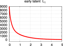
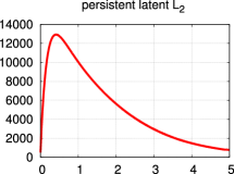
In this section we consider a TB mathematical model proposed in [11], where reinfection and post-exposure interventions for tuberculosis are considered. The model divides the total population into five categories: susceptible ($S$); early latent ($L_{1}$), i.e., individuals recently infected (less than two years) but not infectious; infected ($I$), i.e., individuals who have active TB and are infectious; persistent latent ($L_{2}$), i.e., individuals who were infected and remain latent; and recovered ($R$), i.e., individuals who were previously infected and have been treated. As in [11], we assume that the total population, $N$, with $N=S(t)+L_{1}(t)+I(t)+L_{2}(t)+R(t)$, is constant in time. In other words, we assume that the birth and death rates are equal and there are no TB-related deaths. We introduce a discrete time-delay in the state variable $I$, denoted by $d_{I}$, that represents the delay to diagnosis and commencement of treatment of active TB infection,

$$\begin{cases}\dot{S}(t)=\mu N-\frac{\beta}{N}I(t)S(t)-\mu S(t),\\ \dot{L_{1}}(t)=\frac{\beta}{N}I(t)\left(S(t)+\sigma L_{2}(t)+\sigma_{R}R(t)\right)-\left(\delta+\tau_{1}+\mu\right)L_{1}(t),\\ \dot{I}(t)=\phi\delta L_{1}(t)+\omega L_{2}(t)+\omega_{R}R(t)-\tau_{0}I(t-d_{I})-\mu I(t),\\ \dot{L_{2}}(t)=(1-\phi)\delta L_{1}(t)-\sigma\frac{\beta}{N}I(t)L_{2}(t)-(\omega+\tau_{2}+\mu)L_{2}(t),\\ \dot{R}(t)=\tau_{0}I(t-d_{I})+\tau_{1}L_{1}(t)+\tau_{2}L_{2}(t)-\sigma_{R}\frac{\beta}{N}I(t)R(t)-(\omega_{R}+\mu)R(t)\,.\end{cases}$$ (1)

The initial conditions for system (1) are

$$S(\theta)=\varphi_{1}(\theta),\,L_{1}(\theta)=\varphi_{2}(\theta),\,I(\theta)=\varphi_{3}(\theta),\,L_{2}(\theta)=\varphi_{4}(\theta),\,R(\theta)=\varphi_{5}(\theta),$$ (2)

$-d_{I}\leq\theta\leq 0$, where $\varphi=\left(\varphi_{1},\varphi_{2},\varphi_{3},\varphi_{4},\varphi_{5}\right)^{T}\in C$ with $C$ the Banach space $C\left([-d_{I},0],{\mathbb{R}}^{5}\right)$ of continuous functions mapping the interval $[-d_{I},0]$ into ${\mathbb{R}}^{5}$. From biological meaning, we further assume that $\varphi_{i}(0)>0$ for $i=1,\ldots,5$.

Throughout this paper, we focus on the dynamics of the solutions of (1) in the restricted region

$$\Omega=\left\{(S,L_{1},I,L_{2},R)\in{\mathbb{R}}^{5}_{+0}\,|\,0\leq S+L_{1}+I+L_{2}+R=N\right\}.$$

In this region, the usual local existence, uniqueness and continuation results apply [12, 14]. Hence, a unique solution $\left(S(t),L_{1}(t),I(t),L_{2}(t),R(t)\right)$ of (1) with initial condition (2) exists for all time $t\geq 0$. Consider the solutions of (1) with $(\varphi_{1}(\theta),\ldots,\varphi_{5}(\theta))\in Int\,\Omega$, $i=1,\ldots,5$, for all $\theta\in[-d_{I},0]$. Then the solutions stay in the interior of the region $\Omega$ for all time $t\geq 0$, i.e., the region $\Omega$ is positively invariant with respect to system (1) (see, e.g., [14]).

A mathematical model has a disease free equilibrium if it has an equilibrium point at which the population remains in the absence of the disease [28]. The model (1) has a disease free equilibrium given by $E_{0}=(N,0,0,0,0)$.

The basic reproduction number $R_{0}$ represents the expected average number of new TB infections produced by a single TB active infected individual when in contact with a completely susceptible population [28]. For model (1) it is given by

$$R_{0}=\frac{\beta}{\mu}\frac{\omega_{R}\left(\omega+\tau_{2}+\mu\right)\tau_{1}+\delta\left[\left(\omega_{R}+\mu\right)\left(\phi\mu+\omega\right)+\left(\omega_{R}+\phi\mu\right)\tau_{2}\right]}{\left(\tau_{0}+\mu+\omega_{R}\right)\left(\omega+\tau_{2}+\mu\right)\left(\delta+\tau_{1}+\mu\right)}=\frac{\mathcal{N}}{\mathcal{D}}\,.$$ (3)

Note that in [11] the basic reproduction number is deduced under the assumption that $\tau_{1}=\tau_{2}=0$. The expression (3) generalizes the one given in [11].

3. Stability of the disease free equilibrium

It is important to analyze the stability of the disease free equilibrium, as it indicates whether the population will remain in the absence of the disease, or the disease will persist for all time [28, 29]. System (1) is equivalent to

$$\begin{cases}\dot{S}(t)=\mu N-\frac{\beta}{N}I(t)S(t)-\mu S(t),\\ \dot{L_{1}}(t)=\frac{\beta}{N}I(t)\left(S(t)+\sigma L_{2}(t)+\sigma_{R}(N-S(t)-L_{1}(t)-I(t)-L_{2}(t))\right)\\ \quad\quad-\left(\delta+\tau_{1}+\mu\right)L_{1}(t),\\ \dot{I}(t)=\phi\delta L_{1}(t)+\omega L_{2}(t)+\omega_{R}(N-S(t)-L_{1}(t)-I(t)-L_{2}(t))\\ \quad\quad-\tau_{0}I(t-d_{I})-\mu I(t),\\ \dot{L_{2}}(t)=(1-\phi)\delta L_{1}(t)-\sigma\frac{\beta}{N}I(t)L_{2}(t)-(\omega+\tau_{2}+\mu)L_{2}(t)\,,\end{cases}$$ (4)

where the equation for $R(t)$ is derived from $R(t)=N-S(t)-L_{1}(t)-I(t)-L_{2}(t)$. The disease free equilibrium of system (4) is given by $(S_{0},L_{10},I_{0},L_{20})=(N,0,0,0)$. To discuss its local asymptotic stability, let us consider the coordinate transformation $s(t)=S(t)-\overline{S}$, $l_{1}(t)=L_{1}(t)-\overline{L}_{1}$, $i(t)=I(t)-\overline{I}$, $l_{2}(t)=L_{2}(t)-\overline{L}_{2}$, where $(\overline{S},\overline{L}_{1},\overline{I},\overline{L}_{2})$ denotes any equilibrium of (4). Hence, we have that the corresponding linearized system of (4) is of the form

$$\begin{cases}\dot{s}(t)=-{\frac{\beta\,\overline{I}+\mu\,N}{N}}\,s(t)-\frac{\beta}{N}\,\overline{S}\,i(t)\\[5.69046pt] \dot{l}_{1}(t)=-\frac{\beta}{N}\,\overline{I}\,\left(\sigma_{R}-1\right)\,s(t)-\frac{\beta}{N}\left(\sigma_{R}\,\overline{I}+(\delta+\tau_{1}+\mu)N\right)\,l_{1}(t)\\ \quad\quad\quad-\frac{\beta}{N}\left(-\overline{S}-\sigma\,\overline{L}_{2}-\sigma_{R}(N+\overline{S}+\overline{L}_{1}+2\,\overline{I}+\overline{L}_{2})\right)\,i(t)+{\frac{\beta\,\overline{I}\,\left(\sigma-\sigma_{R}\right)}{N}}\,l_{2}(t)\\[5.69046pt] \dot{i}(t)=-\omega_{R}\,s(t)+\left(\phi\,\delta-\omega_{R}\right)l_{1}(t)-\left(\omega_{R}-\mu\right)i(t)+\left(\omega-\omega_{R}\right)l_{2}(t)-\tau_{0}\,i(t-d_{I})\\[5.69046pt] \dot{l}_{2}(t)=\left(1-\phi\right)\delta\,l_{1}(t)-\frac{\beta}{N}\sigma\,\overline{L}_{2}\,i(t)-\frac{\beta}{N}\left(\sigma\overline{I}+(\omega+\tau_{2}+\mu)N\right)\,l_{2}(t)\,.\end{cases}$$ (5)

We then express system (5) in matrix form as follows:

$$\frac{d}{dt}\left(\begin{array}[]{c}s(t)\\ l_{1}(t)\\ i(t)\\ l_{2}(t)\end{array}\right)=A_{1}\left(\begin{array}[]{c}s(t)\\ l_{1}(t)\\ i(t)\\ l_{2}(t)\end{array}\right)+A_{2}\left(\begin{array}[]{c}s(t-d_{I})\\ l_{1}(t-d_{I})\\ i(t-d_{I}))\\ l_{2}(t-d_{I})\end{array}\right)$$

with $A_{1}$ the $4\times 4$ matrix

$$A_{1}=\left[\begin{array}[]{cccc}-{\frac{\beta\,\overline{I}+\mu\,N}{N}}&0&-{\frac{\beta\,\overline{S}}{N}}&0\\ \vskip 6.0pt plus 2.0pt minus 2.0pt\cr{\frac{\beta\,\overline{I}\,\left(1-\sigma_{R}\right)}{N}}&-{\frac{\beta\,\overline{I}\,\sigma_{R}+c_{1}N}{N}}&{\frac{\beta\,\left(\overline{S}+\sigma\,\overline{L}_{2}+\sigma_{R}(N+\overline{S}+\overline{L}_{1}+2\,\overline{I}+\overline{L}_{2})\right)}{N}}&{\frac{\beta\,\overline{I}\,\left(\sigma-\sigma_{R}\right)}{N}}\\ \vskip 6.0pt plus 2.0pt minus 2.0pt\cr-\omega_{R}&\phi\,\delta-\omega_{R}&-\omega_{R}-\mu&\omega-\omega_{R}\\ \vskip 6.0pt plus 2.0pt minus 2.0pt\cr 0&-\left(-1+\phi\right)\delta&-{\frac{\sigma\,\beta\,\overline{L}_{2}}{N}}&-{\frac{\beta\,\overline{I}\,\sigma+c_{2}N}{N}}\end{array}\right],$$

where $c_{1}=\delta+\tau_{1}+\mu$ and $c_{2}=\omega+\tau_{2}+\mu$, and $A_{2}$ the $4\times 4$ diagonal matrix $A_{2}=\textrm{diag}(0,0,-\tau_{0},0)$. The transcendental characteristic equation of system (5) is defined by $\Delta(\lambda)=\det\left(\lambda I-A_{1}-{\rm e}^{-\lambda d_{I}}A_{2}\right)=0$ and is given by

$$\Delta(\lambda)=P(\lambda)+Q(\lambda)=0,$$ (6)

where

$$\begin{split}P(\lambda)&=\lambda^{4}+a_{3}\lambda^{3}+a_{2}\lambda^{2}+a_{1}\lambda+a_{0},\\ Q(\lambda)&=\tau_{0}\left(\lambda+\mu\right)\left(\lambda+c_{1}\right)\left(\lambda+c_{2}\right)\left({\rm e}^{-\lambda d_{I}}-1\right),\end{split}$$

with $a_{0}=\mathcal{D}-\mathcal{N}$,

$$\begin{split}a_{1}&=\frac{2}{\mu}\,\mathcal{D}+\mu^{2}(c_{1}+c_{2}+c_{4})-c_{4}c_{5}c_{6}-\beta(\tau_{1}\omega_{R}+\omega\delta+\delta\phi(\omega_{R}+\tau_{2}+2\mu)),\\ a_{2}&=c_{4}c_{5}+3\,\mu(c_{1}+c_{2}+c_{4})+c_{6}(c_{4}+c_{5})-\beta\,\phi\,\delta\,,\\ a_{3}&=c_{1}+c_{2}+c_{3}+\mu,\end{split}$$

and $c_{3}=\omega_{R}+\tau_{0}+\mu$, $c_{4}=\tau_{0}+\omega_{R}$, $c_{5}=\tau_{2}+\omega$, $c_{6}=\delta+\tau_{1}$.

Remark 1.

For any $d_{I}\geq 0$ and $a_{3}>0$, if $R_{0}<1$, then $a_{0}>0$.

Recall that an equilibrium point is asymptotically stable if all roots of the corresponding characteristic equation have negative real parts [1].

Lemma 3.1.

If $R_{0}>1$, then the disease free equilibrium $E_{0}$ is unstable for any $d_{I}\geq 0$.

Proof.

The characteristic equation (6) satisfies $\Delta(0)=\mathcal{D}-\mathcal{N}$. Assuming $R_{0}>1$, then $\Delta(0)<0$. Since $\lim_{\lambda\to+\infty}\Delta(\lambda)=+\infty$, there exists at least one positive root of (6). ∎

Lemma 3.2.

If (i) $R_{0}<1$, (ii) $a_{1}>0$, (iii) $a_{2}>0$, (iv) $a_{3}a_{2}>a_{1}$, and (v) $a_{3}a_{2}a_{1}>a_{1}^{2}+a_{3}^{2}a_{0}$, then the disease free equilibrium $E_{0}$ is locally asymptotically stable for $d_{I}=0$.

Proof.

When $d_{I}=0$, the associated transcendental characteristic equation (6) of system (5) at $(N,0,0,0)=(\overline{S},\overline{L}_{1},\overline{I},\overline{L}_{2})$ becomes $\Delta(\lambda)=P(\lambda)=0$. Using the Routh–Hurwitz criterion for fourth-order polynomials, all the roots of $P(\lambda)$ have negative real part if all coefficients satisfy $a_{n}>0$ for $n=0,\ldots,3$, $a_{3}a_{2}>a_{1}$, and $a_{3}a_{2}a_{1}>a_{1}^{2}+a_{3}^{2}a_{0}$. ∎

In the case $d_{I}>0$, by Rouché’s theorem [8], if instability occurs for a particular value of the delay $d_{I}$, then a characteristic root of (6) must intersect the imaginary axis. Our aim is to prove that the polynomial (6) does not have purely imaginary roots for all positive delays (see, e.g., [2, 7]). The complex $i\,b$, $b>0$, is a root of (6) if and only if ${b}^{4}-ia_{3}{b}^{3}-a_{2}{b}^{2}+ia_{1}b+a_{0}+\tau_{0}\left(ib+\mu\right)\left(ib+c_{1}\right)\left(ib+c_{2}\right)\left({{\rm e}^{-ib\,d_{I}}}-1\right)=0$. By using Euler’s formula $\exp^{-ibd_{I}}=\cos(bd_{I})-i\sin(bd_{I})$, and by separating real and imaginary parts, we have

$$a_{3}{b}^{3}+\tau_{0}bc_{1}c_{2}-a_{1}b-\tau_{0}{b}^{3}+\tau_{0}\mu c_{1}b+\tau_{0}\mu bc_{2}=A\cos(bd_{I})-B\sin(bd_{I})\\ -{b}^{4}+a_{2}{b}^{2}-\tau_{0}{b}^{2}c_{1}-a_{0}-\tau_{0}{b}^{2}c_{2}-\mu\tau_{0}{b}^{2}+\tau_{0}\mu c_{1}c_{2}=A\sin(bd_{I})+B(\cos(bd_{I}))$$

with $A=\tau_{0}b(c_{1}c_{2}-{b}^{2}+\mu(c_{1}+c_{2}))$ and $B=\tau_{0}(\mu c_{1}c_{2}-{b}^{2}(\mu+c_{1}+c_{2}))$. Adding up the squares of both equations, we obtain that

$${b}^{8}+\alpha_{3}{b}^{6}+\alpha_{2}{b}^{4}+\alpha_{1}{b}^{2}+\alpha_{0}=0,$$ (7)

where $\alpha_{0}=a_{0}(a_{0}-2\,\mu\,\tau_{0}\,c_{1}\,c_{2})$,

$$\begin{split}\alpha_{1}&=2\tau_{0}(\mu(a_{0}+a_{2}c_{1}\,c_{2}-a_{1}(c_{1}+c_{2}))+a_{0}(c_{1}+c_{2})-a_{1}c_{1}c_{2})-2a_{2}a_{0}+a_{1}^{2},\\ \alpha_{2}&=2\tau_{0}\left(\mu(a_{3}(c_{1}+c_{2})-a_{2}-c_{1}c_{2})-a_{2}(c_{1}+c_{2})+a_{3}c_{1}c_{2}+a_{1}\right)+2a_{0}+a_{2}^{2}\\ &\hskip 11.38109pt-2a_{3}a_{1},\\[-0.56905pt] \alpha_{3}&=2\tau_{0}(\mu+c_{1}+c_{2})+{a_{3}}^{2}-2(a_{3}\tau_{0}+a_{2}).\end{split}$$

Let $z=b^{2}$. Then (7) becomes

$${z}^{4}+\alpha_{3}{z}^{3}+\alpha_{2}{z}^{2}+\alpha_{1}{z}+\alpha_{0}=0.$$ (8)

By the Routh–Hurwitz criterion, (8) has no positive real roots if $\alpha_{i}>0$, $i=0,\ldots,3$, $\alpha_{3}\alpha_{2}>\alpha_{1}$, and $\alpha_{3}\alpha_{2}\alpha_{1}>\alpha_{1}^{2}+\alpha_{3}^{2}\alpha_{0}$.

For the parameter values of Table 1 and $\beta=40$ ($R_{0}=0.880827$), the Routh–Hurwitz criterion does not hold. In fact, equation (8) takes the form

$${z}^{4}+241.429794{z}^{3}+31.065028{z}^{2}-221.270089{z}-0.037233=0$$ (9)

and we immediately see that the coefficient $\alpha_{1}=-221.270089$ is not positive. Moreover, the roots of equation (9) are approximately $0.89$, $-0.00017$, $-1.03$, $-241.30$, therefore there exists a positive imaginary root given by $0.89i$. Thus, there exists at least one time delay such that the disease free equilibrium is unstable. We have just proved the following result.

Lemma 3.3.

Let $R_{0}<1$. Then there exists at least one positive time delay $d_{I}>0$ such that the disease free equilibrium $(N,0,0,0)$ is unstable.

Remark 2.

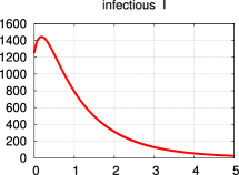
Observe that there may exist specific time delays for which the disease free equilibrium $(N,0,0,0)$ is locally asymptotically stable when $R_{0}<1$. As we show next, this is the case for the time delay $d_{I}=0.1$. Indeed, consider the parameter values of Table 1 and $\beta$ such that $R_{0}<1$. For example, let $\beta=40$, for which $R_{0}=0.880827$. The results are given in Figure 1, where to compute the trajectories we have used the Matlab routine dde23, which solves delay differential equations with constant delays. For the theoretical results that underlie this solver we refer to [21].

(a) State variables

(b) Infected active TB ($T=100$)

Figure 1. Disease free equilibrium with basic reproduction number $R_{0}=0.88$ ($\beta=40$, $d_{I}=0.1$ and the other values from Table 1).

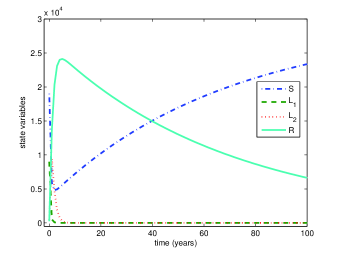
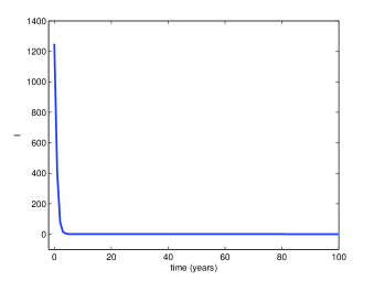
The characteristic equation (6) takes the form $\chi(\lambda)=0$ with

$$\begin{split}\chi(\lambda)={\lambda}^{4}&+17.057363\,{\lambda}^{3}+20.733305\,{\lambda}^{2}+4.489748\,\lambda+0.048755\\ &+2\,\left(\lambda+{\frac{1}{70}}\right)\left(\lambda+{\frac{981}{70}}\right)\left(\lambda+1.014486\right)\left({{\rm e}^{-\lambda\,0.1}}-1\right)\,.\end{split}$$

The derivative $\chi^{\prime}(\lambda)$ has exactly four zeros: $\bar{\lambda}_{1}=-21.408183$, $\bar{\lambda}_{2}=-12.680307$, $\bar{\lambda}_{3}=-0.748206$, and $\bar{\lambda}_{4}=-0.151719$. For all $\lambda\in]-\infty,\bar{\lambda}_{1}[$ one has $\chi^{\prime}(\lambda)>0$ and since $\lim_{\lambda\rightarrow-\infty}\chi(\lambda)=-\infty$ and $\chi(\bar{\lambda}_{1})>0$, we conclude that there exists a unique $\lambda_{1}$ in the interval $]-\infty,\bar{\lambda}_{1}[$ such that $\chi(\lambda_{1})=0$. Analogously, we prove that there exists exactly five roots of $\chi(\lambda)=0$: $\lambda_{1}=-23.481727$, $\lambda_{2}=-18.106597$, $\lambda_{3}=-1.024343$, $\lambda_{4}=-0.320880$, $\lambda_{5}=-0.011482$. We conclude that there are no positive real roots and that the disease free equilibrium $(N,0,0,0)$ is locally asymptotically stable for $d_{I}=0.1$ and the considered parameter values.

In this paper we assume that the time delay $d_{I}$ associated to the diagnosis of active TB is equal to 0.1, that is, 36.5 days. This value makes sense from the epidemiological point of view, since it fits in the intervals available in the literature for the delay in the diagnosis of active TB. For instance, in [24] the reported overall patient delay is similar to the health system delay for diagnosis of active TB, 31.03 and 27.2 days, respectively. The average (median or mean) patient delay and health system delay range from 4.9 to 162 days and 2 to 87 days, respectively, in both low and middle income countries and high income countries.

4. Stability of the endemic equilibrium

System (1) has an unique endemic equilibrium such that $I(t)>0$ for any $t>0$. The analytic expression is cumbersome and not useful for our purposes. Consider the parameter values from Table 1 with $\beta=100$. Then the basic reproduction number is $R_{0}=2.202067$. The endemic equilibrium $E^{*}$ is given by $I=11.006448$, $L_{1}=36.111397$, $L_{2}=402.155827$, $S=8407.668384$. The matrices $A_{1}$ and $A_{2}$ associated to the linearized system (5) at the endemic equilibrium $E^{*}$ are computed as

$$A_{1}=\left[\begin{array}[]{cccc}-0.050974&0&-28.025561&0\\ \vskip 6.0pt plus 2.0pt minus 2.0pt\cr 0.027516&-14.023458&45.970734&0\\ \vskip 6.0pt plus 2.0pt minus 2.0pt\cr-0.000020&0.599980&-0.014306&0.000180\\ \vskip 6.0pt plus 2.0pt minus 2.0pt\cr 0&11.400000&-0.335130&-1.023658\end{array}\right]$$

and $A_{2}=\textrm{diag}(0,0,-2,0)$. The transcendental characteristic equation is given by

$${\lambda}^{4}+15.112395\,{\lambda}^{3}-12.243801\,{\lambda}^{2}-28.331139\,\lambda-0.966336\\ +\left(30.196179\,{\lambda}^{2}+30.244462\,\lambda+2\,{\lambda}^{3}+1.463482\right){{\rm e}^{-\lambda\,{\it d_{I}}}}=0\,.$$ (10)

When $d_{I}=0$, we have the following characteristic equation:

$${\lambda}^{4}+17.112395\,{\lambda}^{3}+17.952378\,{\lambda}^{2}+1.913323\,\lambda+0.497146=0\,.$$ (11)

The roots of (11) are $-1.029896$, $-15.997555$, $-0.042472-0.168435\,i$, $-0.042472+0.168435\,i$. All the roots of (11) have negative real part, thus the endemic equilibrium $E^{*}$ is asymptotical stable. Consider now the case $d_{I}>0$ and suppose that (10) has a purely imaginary root $b\,i$, with $b>0$. Separating the real and imaginary parts in (10), we have

$${b}^{8}+281.828573\,{b}^{6}-51.906667\,{b}^{4}-1.236501\,{b}^{2}-0.000246=0\,.$$ (12)

It is easy to verify that $b=0.453220$ is a root of equation (12). Thus, by Rouché’s theorem, there exists at least a time delay $d_{I}>0$ such that the endemic equilibrium $E^{*}$ is unstable. In the specific case $d_{I}=0.1$, the characteristic equation is given by

$${\lambda}^{4}+15.112395\,{\lambda}^{3}-12.243801\,{\lambda}^{2}-28.331139\,\lambda-0.966336\\ +\left(2\,{\lambda}^{3}+30.196179\,{\lambda}^{2}+30.244462\,\lambda+1.463482\right){{\rm e}^{-0.1\,\lambda}}=0\,.$$ (13)

Similarly to Remark 2, it follows from Bolzano’s theorem and the monotonicity of the characteristic function associated to (13) that all roots of equation (13) have a negative real part. Therefore, the endemic equilibrium $E^{*}$ is locally asymptotically stable for $d_{I}=0.1$ and $R_{0}>1$.

Symbol	Description	Value
$\beta$	Transmission coefficient	$\in[50,150]$
$\mu$	Death and birth rate	$1/70\,yr^{-1}$
$\delta$	Rate at which individuals leave $L_{1}$	$12\,yr^{-1}$
$\phi$	Proportion of individuals going to $I$	$0.05$
$\omega$	Endogenous reactivation rate for persistent latent infections	$0.0002\,yr^{-1}$
$\omega_{R}$	Endogenous reactivation rate for treated individuals	$0.00002\,yr^{-1}$
$\sigma$	Factor reducing the risk of infection as a result of acquired
	immunity to a previous infection for $L_{2}$	$0.25$
$\sigma_{R}$	Rate of exogenous reinfection of treated patients	0.25
$\tau_{0}$	Rate of recovery under treatment of active TB	$2\,yr^{-1}$
$\tau_{1}$	Rate of recovery under treatment of early latent individuals $L_{1}$	$2\,yr^{-1}$
$\tau_{2}$	Rate of recovery under treatment of persistent latent individuals $L_{2}$	$1\,yr^{-1}$
$N$	Total population	$30,000$
$T$	Total simulation duration	$5$ $yr$
$\epsilon_{1}$	Efficacy of treatment of early latent $L_{1}$	$0.5$
$\epsilon_{2}$	Efficacy of treatment of persistent latent TB $L_{2}$	$0.5$

Table 1. Parameter values.

5. Optimal control of a tuberculosis model with state and control delays

We now consider the TB model (1) with a time delay in the state variable $I(t)$ and introduce two control functions $u_{1}(\cdot)$ and $u_{2}(\cdot)$ and two real positive model constants $\epsilon_{1}$ and $\epsilon_{2}$. The control $u_{1}$ represents the effort on early detection and treatment of recently infected individuals $L_{1}$ and the control $u_{2}$ represents the application of chemotherapy or post-exposure vaccine to persistent latent individuals $L_{2}$. The parameters $\epsilon_{i}\in(0,1)$, $i=1,2$, measure the effectiveness of the controls $u_{i}$, $i=1,2$, respectively, i.e., these parameters measure the efficacy of post-exposure interventions for early and persistent latent TB individuals, respectively. Since after TB infection the human immune system can take from 2 to 8 weeks to react, it takes at least the same time to detect the infection by the medical test [33]. Hence, we introduce a time delay $d_{u_{1}}$ in the control $u_{1}$ which represents the delay in the diagnosis of latent TB and commencement of latent TB treatment. The prophylactic treatment of persistent latent individuals may also suffer from a delay due to personal reasons of the patient, who may be resistant to treatment having spent more than two years with latent infection without passing to active disease, or the delay may be caused by priorities given to early latent and active infectious individuals from the health care system. Based on these facts, for numerical simulations we shall consider the following delays with bounds on the control delays:

$$d_{I}=0.1,\quad d_{u_{1}},\,d_{u_{2}}\in[0.05,0.2]\,.$$ (14)

The resulting model is given by the following system of nonlinear ordinary delay differential equations:

$$\begin{cases}\dot{S}(t)=\mu N-\frac{\beta}{N}I(t)S(t)-\mu S(t),\\[0.85358pt] \dot{L_{1}}(t)=\frac{\beta}{N}I(t)\left(S(t)+\sigma L_{2}(t)+\sigma_{R}R(t)\right)-\left(\delta+\tau_{1}+\epsilon_{1}u_{1}(t-d_{u_{1}})+\mu\right)L_{1}(t),\\[0.85358pt] \dot{I}(t)=\phi\delta L_{1}(t)+\omega L_{2}(t)+\omega_{R}R(t)-\tau_{0}I(t-d_{I})-\mu I(t),\\[0.85358pt] \dot{L_{2}}(t)=(1-\phi)\delta L_{1}(t)-\sigma\frac{\beta}{N}I(t)L_{2}(t)-(\omega+\epsilon_{2}u_{2}(t-d_{u_{2}})+\tau_{2}+\mu)L_{2}(t).\end{cases}$$ (15)

Recall that the recovered population is determined by $R(t)=N-(S(t)+L_{1}(t)+I(t)+L_{2}(t))$, which formally gives the equation

$$\dot{R}(t) = \tau_{0}I(t-d_{I})+(\tau_{1}+\epsilon_{1}u_{1}(t-d_{u_{1}}))L_{1}(t)+(\tau_{2}+\epsilon_{2}u_{2}(t-d_{u_{2}}))L_{2}(t)$$

$$-\sigma_{R}\frac{\beta}{N}I(t)R(t)-(\omega_{R}+\mu)R(t)\,.$$

Note, however, that this equation is not needed in the subsequent optimal control computations. We prescribe the following initial conditions for the state variables $(S,L_{1},L_{2})$ and, due to the delays, initial functions for the state variable $I$ and controls $u_{1}$ and $u_{2}$:

$$\begin{array}[]{l}S(0)=(76/120)N,\;L_{1}(0)=(36/120)N,\;L_{2}(0)=(2/120)N,\;R(0)=(1/120)N,\\[1.42262pt] I(t)=(5/120)N\;\;\mbox{for}\;-d_{I}\leq t\leq 0,\;u_{k}(t)=0\;\;\mbox{for}\;-d_{u_{k}}\leq t<0\;\;(k=1,2).\end{array}$$ (16)

In the case $d_{u_{1}}=d_{u_{2}}=0$ of no control delays, the last condition is void. The following box constraints are imposed on the control variables:

$$0\leq u_{k}(t)\leq 1\quad\forall\;t\in[0,T]\quad(k=1,2).$$ (17)

Let us denote the state and control variable of the control system (15), respectively, by $x=(S,L_{1},I,L_{2})\in\mathbb{R}^{4}$ and $u=(u_{1},u_{2})\in\mathbb{R}^{2}$. We shall consider two types of objectives: either the $L^{1}$–type objective

$$J_{1}(x,u)=\int_{0}^{T}(I(t)+L_{2}(t)+W_{1}\,u_{1}(t)+W_{2}\,u_{2}(t))\,dt\,,$$ (18)

which is linear in the control variable $u$, or the $L^{2}$–type objective

$$J_{2}(x,u)=\int_{0}^{T}(I(t)+L_{2}(t)+W_{1}\,u_{1}^{2}(t)+W_{2}\,u_{2}^{2}(t))\,dt\,,$$ (19)

which is quadratic in the control variable. In both objectives, $W_{1}>0$, $W_{2}>0$ are appropriate weights to be chosen later. $L^{2}$-type functionals like (19) are often used in economics to describe, e.g., productions costs, but are not appropriate in a biological framework; cf. the remarks in [20]. The $L^{1}$ functional $J_{1}(x,u)$ incorporates the total amount of drug used as a penalty and thus appears to be more realistic. For that reason, we shall mainly focus on the functional $J_{1}(x,u)$.

The optimal control problem then is defined as follows: determine a control function $u=(u_{1},u_{2})\in L^{1}([0,T],\mathbb{R}^{2})$ that minimizes either the cost functional $J_{1}(x,u)$ in (18) or $J_{2}(x,u)$ in (19) subject to the dynamic constraints (15), initial conditions (16) and control constraints (17). Necessary optimality conditions for optimal control problems with multiple time delays in control and state variables may be found, e.g., in [10]. Here, we discuss the Maximum Principle in order to display the controls and the switching functions in a convenient way. To define the Hamiltonian for the delayed control problem, we introduce the delayed state variable $y_{3}(t)=x_{3}(t-d_{I})=I(t-d_{I})$ and the delayed control variables $v_{k}(t)=u_{k}(t-d_{u_{1}})$, $k=1,2$. Using the adjoint variable $\lambda=(\lambda_{S},\lambda_{L_{1}},\lambda_{I},\lambda_{L_{2}})\in\mathbb{R}^{4}$, the Hamiltonian for the objective $J_{1}$ and the control system (15) is given by

$$\begin{array}[]{l}H(x,y_{3},\lambda,u_{1},u_{2},v_{1},v_{2})=-(I+L_{2}+W_{1}u_{1}+W_{2}u_{2})+\lambda_{S}(\mu N-\frac{\beta}{N}IS-\mu S)\\[2.84526pt] \quad+\lambda_{L_{1}}(\frac{\beta}{N}(S+\sigma L_{2}+\sigma_{R}R)-(\delta+\tau_{1}+\epsilon_{1}v_{1}+\mu)L_{1})\\[2.84526pt] \quad+\lambda_{I}(\phi\delta L_{1}+\omega L_{2}+\omega_{R}R-\tau_{0}y_{3}-\mu I)\\[2.84526pt] \quad+\lambda_{L_{2}}((1-\phi)\delta L_{1}-\sigma\frac{\beta}{N}IL_{2}-(\omega+\epsilon_{2}v_{2}+\tau_{2}+\mu)L_{2}).\end{array}$$

We obtain the adjoint equations $\dot{\lambda}_{S}(t)=-H_{S}[t]$, $\dot{\lambda}_{L_{1}}(t)=-H_{L_{1}}[t]$, $\dot{\lambda}_{L_{2}}(t)=-H_{L_{2}}[t]$, and $\dot{\lambda}_{I}(t)=-H_{I}[t]+\chi_{\,[0,T-d_{I}]}\,H_{y_{3}}[t+d_{I}]$, where subscripts denote partial derivatives and $\chi_{\,[0,T-d_{I}]}$ is the characteristic function in the interval $[0,T-d_{I}]$ [10]. Note that only the equation for $\dot{\lambda}_{I}(t)$ contains the advanced time $t+d_{I}$. Since the terminal state $x(T)$ is free, the transversality conditions are

$$\lambda_{S}(T)=\lambda_{L_{1}}(T)=\lambda_{I}(T)=\lambda_{L_{2}}(T)=0.$$ (20)

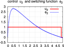
To characterize the optimal controls $u_{1}$ and $u_{2}$, we introduce the following switching functions for $k=1,2$:

$$\begin{array}[]{rl}\phi_{k}(t)&=\;H_{u_{k}}[t]+\chi_{\,[0,T-d_{u_{k}}]}(t+d_{u_{k}})\,H_{v_{k}}[t+d_{u_{k}}]\\[2.84526pt] &=\;\left\{\begin{array}[]{lcl}-W_{k}-\epsilon_{k}\lambda_{L_{k}}(t+d_{u_{k}})L_{k}(t+d_{u_{k}})&\mbox{for}&0\leq t\leq T-d_{u_{k}},\\[2.84526pt] -W_{k}&\mbox{for}&T-d_{u_{k}}\leq t\leq T.\end{array}\right.\end{array}$$ (21)

Then the maximum condition for the optimal controls $u_{1}(t)$, $u_{2}(t)$ is equivalent to the maximization $\,\phi_{k}(t)u_{k}(t)=\max_{\,0\leq u_{k}\leq 1}\;\phi_{k}(t)u_{k}$, $k=1,2$, which gives the control law

$$u_{k}(t)=\left\{\begin{array}[]{rcl}1&&\mbox{if}\quad\phi_{k}(t)>0,\\[2.84526pt] 0&&\mbox{if}\quad\phi_{k}(t)<0,\\[2.84526pt] {\rm singular}&&\mbox{if}\quad\phi_{k}(t)=0\;\;\mbox{on}\;I_{s}\subset[0,T],\end{array}\right.\quad k=1,2.$$ (22)

We do not discuss singular controls further, since both in the non-delayed and the delayed control problem we did not find singular arcs. In view of the transversality conditions (20), the terminal value of the switching function is $\phi_{k}(T)=-W_{k}$ for $k=1,2$. Hence, we may conclude from the control law (22) that $u_{1}(t)=u_{2}(t)=0$ holds on a terminal interval.

6. Numerical results for the non-delayed and the delayed optimal control problem

We choose the numerical approach “First Discretize then Optimize” to solve both the non-delayed and delayed optimal control problem. The discretization of the control problem on a fine grid leads to a large-scale nonlinear programming problem (NLP) that can be conveniently formulated with the help of the Applied Modeling Programming Language AMPL [9]. AMPL can be linked to several powerful optimization solvers. We use the Interior-Point optimization solver IPOPT developed by Wächter and Biegler [30]. Details of discretization methods for delayed control problems may be found in [10]. The subsequent computations for the terminal time $t_{f}=5$ have been performed with $N=2500$ to $N=5000$ grid points using the trapezoidal rule as integration method. Choosing the error tolerance $tol=10^{-10}$ in IPOPT, we can expect that the state variables are correct up to $7$ or $8$ decimal digits. Since Lagrange multipliers are computed a posteriori in IPOPT, we cannot expect more than 6 correct decimal digits in the adjoint variables.

Also, the control package NUDOCCCS developed by Büskens [3] (cf. also [4]) provides a highly efficient method for solving the discretized control problem, because it allows to implement higher order integration methods. However, so far NUDOCCCS can only be implemented for non-delayed control problems. For the non-delayed TB control problem, we obtained only bang-bang controls. An important feature of NUDOCCCS is the fact that it provides an efficient method for optimizing the switching times of bang-bang controls using the arc-parametrization method [16]. This approach is called the Induced Optimization Problem (IOP) for bang-bang controls. NUDOCCCS then allows for a check of second-order sufficient conditions of the IOP, whereby the second-order sufficient conditions for bang-bang controls can be verified with high accuracy; cf. [16, 17].

6.1. Optimal control solution of the non-delayed TB model

First, we consider the optimal control of non-delayed TB model, where formally we put $d_{I}=d_{u_{1}}=d_{u_{2}}=0$. The numerical solutions serve as reference solutions, which later will be compared with the solutions to the delayed control problem. We choose the weights $W_{1}=W_{2}=50$ in the objective (18) and the parameter $\beta=100$ ($R_{0}=2.2$) in Table 1. The discretization approach shows that controls $u_{k}(t)$ are bang-bang and with only one switch at $t_{k}$, $k=1,2$:

$$u_{k}(t)=\left\{\begin{array}[]{rcl}1&\quad\mbox{for}&0\leq t\leq t_{k},\\ 0&\quad\mbox{for}&t_{k}<t\leq T,\end{array}\right.\quad k=1,2.$$ (23)

To obtain a refined solution, we solve the IOP with respect to the switching times $t_{1}$ and $t_{2}$ using the arc-parametrization method [16] and the code NUDOCCCS [3]. We get the following numerical results:

$$\begin{array}[]{rclrclrcl}J_{1}(x,u)&=&28390.73,&\quad t_{1}&=&3.677250,&\quad t_{2}&=&4.866993,\\ S(T)&=&1034.634,&\quad L_{1}(T)&=&53.59586,&\quad I(T)&=&25.89556,\\ L_{2}(T)&=&780.7667,&\quad R(T)&=&28105.11.\end{array}$$ (24)

The initial value of the adjoint variable $\lambda=(\lambda_{s},\lambda_{L_{1}},\lambda_{I},\lambda_{L_{2}})$ is computed as

$$\lambda(0)=(0.376159,0.452761,4.03059,0.394839).$$

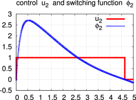
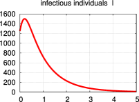
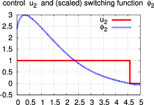
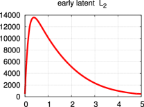
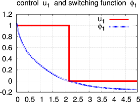
The control and state trajectories are displayed in Figure 2.

Figure 2. Optimal control and state variables of the non-delayed TB model with $L^{1}$ objective (18) and weights $W_{1}=W_{2}=50$. Top row: (a) control $u_{1}$ (23) and (scaled) switching function $\phi_{1}$ (21) satisfying the control law (22) for $k=1$, (b) susceptible individuals $S$ and recovered individuals $R$, (c) infectious individuals $I$. Bottom row: (a) control $u_{2}$ (23) and (scaled) switching function $\phi_{2}$ (21) satisfying the control law (22) for $k=2$, (b) early latent $L_{1}$, (c) persistent latent $L_{2}$.

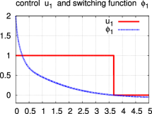
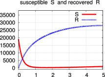
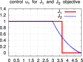
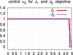
The Hessian $HessL$ of the Lagrangian for the IOP is positive definite: $HessL=\left(\begin{array}[]{ll}453.98&387.42\\ 387.42&385.69\end{array}\right)>0$. It can be seen from Figure 2, top row (a) and bottom row (a), that the switching functions satisfy the strict bang-bang property (cf. [16, 17]) corresponding to the Maximum Principle: $\phi_{k}(t)>0$ for $0\leq t<t_{k}$, $\dot{\phi}_{k}(t_{k})<0$, $\phi_{k}(t)<0$ for $t_{k}<t\leq T\,(k=1,2)$. Hence, the bang-bang controls (23) characterized by the data (24) satisfies the second-order sufficient conditions in [17, Chap. 7] and thus provides a strict strong minimum. Figure 3 displays the comparison of the optimal controls for the functionals $J_{1}(x,u)$ (18) and $J_{2}(x,u)$ (19). The state variables are nearly identical, since the control variables differ only a terminal interval. Also the objective values are very close: $J_{1}(x,u)=28390.73$, $J_{2}(x,u)=28382.37$. Note that the controls for $J_{2}(x,u)$ are continuous, since the strict Legendre–Clebsch condition holds and the Hamiltonian has a unique minimum. The proof, that second-order sufficient conditions (SSC) are satisfied for the controls corresponding to $J_{2}(x,u)$, is quite elaborated since it requires to test whether an associated matrix Riccati equation has a bounded solution; cf. [17].

Figure 3. Comparison of controls $u_{1}$ and $u_{2}$ for the $L^{1}$-type objective (18) and $L^{2}$-type objective (19) with weights $W_{1}=W_{2}=50$.

When we increase the weights $W_{1}$ and $W_{2}$, the control $u_{1}$ stays to be bang-bang with only one switching time which gets smaller, whereas the control $u_{2}$ may have an additional zero arc at the beginning. E.g., for $W_{1}=W_{2}=150$ we obtain the controls

$$(u_{1}(t),u_{2}(t))=\left\{\begin{array}[]{rcl}(1,0)&\quad\mbox{for}&0\leq t\leq t_{1},\\ (1,1)&\quad\mbox{for}&t_{1}<t\leq t_{2},\\ (0,1)&\quad\mbox{for}&t_{2}<t\leq t_{3},\\ (0,0)&\quad\mbox{for}&t_{3}<t\leq T,\end{array}\right.\quad k=1,2.$$

The objective value and the switching times are computed as $J_{1}(x,u)=29175.97$, $t_{1}=0.00260$, $t_{2}=2.662$, and $t_{3}=4.633$. The optimal controls are shown in Figure 4.

Figure 4. Optimal controls $u_{1}$ and $u_{2}$ for the $L^{1}$-type objective (18) with weights $W_{1}=W_{2}=150$.

6.2. Optimal control solution of the TB model with control and state delays

To see more distinctively the difference between delayed and non-delayed solutions, we consider state and control delays with values at their upper bounds in (14), that is, $d_{I}=0.1$, $d_{u_{1}}=0.2$, and $d_{u_{2}}=0.2$. Again, we choose the weights $W_{1}=W_{2}=50$ in the objective (18) and the parameter $\beta=100$ in Table 1, for which $R_{0}=2.2$. The discretization approach with $N=5000$ grid points and the trapezoidal rule as integration method yields the following bang-bang controls with only one switch as in the non-delayed case:

$$u_{k}(t)=\left\{\begin{array}[]{rcl}1&\mbox{for}&0\leq t\leq t_{k},\\ 0&\mbox{for}&t_{k}<t\leq T,\end{array}\right.\quad k=1,2.$$ (25)

We obtain the numerical results $J_{1}(x,u)=26784.60$, $t_{1}=3.108$, $t_{2}=4.581$, $S(T)=1234.598$, $L_{1}(T)=24.93928$, $I(T)=11.71451$, $L_{2}(T)=469.8865$, and $R(T)=28258.86$. However, in contrast to the non-delayed case, we are not able to optimize the switching times directly because the time-transformation in the arc-parametrization method [16] cannot be applied to the delayed problem. The initial value of the adjoint variable is computed as $\lambda(0)=(0.3789,0.4682,3.6412,0.4263)$. When comparing the results for the delayed problem with those in (24) for the non-delayed problem, we notice the surprising fact that the terminal values $L_{1}(T)$, $I(T)$, $L_{2}(T)$ and the switching times $t_{1}$, $t_{2}$ are significantly smaller in the delayed problem on the expense that the terminal value $S(T)$ is significantly higher.

Figure 5. Optimal control and state variables of the delayed TB model with $L^{1}$-objective (18), $W_{1}=W_{2}=50$ and delays $d_{I}=0.1,d_{u_{1}}=d_{u_{2}}=0.2$. Top row: (a) control $u_{1}$ (25) and (scaled) switching function $\phi_{1}$ (21) satisfying the control law (22) for $k=1$, (b) susceptible individuals $S$ and recovered individuals $R$, (c) infectious individuals $I$. Bottom row: (a) control $u_{2}$ (25) and (scaled) switching function $\phi_{2}$ (21) satisfying the control law (22) for $k=2$, (b) early latent $L_{1}$, (c) persistent latent $L_{2}$.

As in the non-delayed problem, the switching functions satisfy the strict bang-bang property related to the Maximum Principle:

$$\phi_{k}(t)>0\quad\mbox{for}\;\;0\leq t<t_{k}\,,\quad\dot{\phi}_{k}(t_{k})<0\,,\quad\phi_{k}(t)<0\quad\mbox{for}\;\;t_{k}<t\leq T\;\;(k=1,2).$$

However, we are not aware in the literature of any type of sufficient conditions which could be applied to the extremal solution shown in Figure 5.

We also compared the extremal solutions for the $L^{1}$-type objective (18) and the $L^{2}$-type objective (19). Since the controls are very similar to those in Figure 3, they are not displayed here. Figure 6 shows the extremal controls for the $L^{1}$-objective (18) for the increased weights $W_{1}=W_{2}=150$.

Figure 6. Extremal controls for the delayed TB model with $L^{1}$ objective (18), $W_{1}=W_{2}=150$ and delays $d_{I}=0.1$, $d_{u_{1}}=d_{u_{2}}=0.2$. (a) control $u_{1}$ (25) and (scaled) switching function $\phi_{1}$ (21) satisfying the control law (22) for $k=1$, (b) control $u_{2}$ (25) and (scaled) switching function $\phi_{2}$ (21) satisfying the control law (22) for $k=2$.

The most significant influence on the optimal controls is exerted by the transmission coefficient $\beta$.

Figure 7. Comparison of extremal controls for parameters $\beta=50$ and $\beta=150$ in the delayed TB model with $L^{1}$ objective (18), weights $W_{1}=W_{2}=150$ and delays $d_{I}=0.1,d_{u_{1}}=d_{u_{2}}=0.2$.

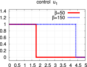
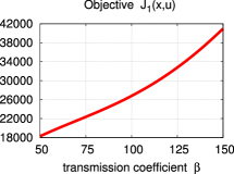
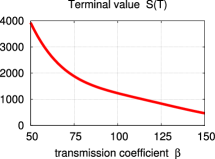
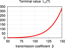
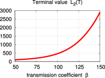
It can be clearly seen that the increase of the transmission coefficient $\beta$ triggers a substantial increase in the switching times $t_{k}$ of the bang-bang controls $u_{k}$ for $k=1,2$ (cf. Figure 7) as could be expected from the equation for $\dot{S}$. Let us perform in this case a more detailed sensitivity analysis of the trajectories with respect to the parameter $\beta\in[50,150]$. We compute the extremal solutions for a sufficiently fine grid of parameters $\beta\in[50,150]$ by a homotopy method and plot the objective $J_{1}(x,u)$ and the terminal state $(S(T),L_{1}(T),I(T),L_{2}(T),R(T))$ as a function of $\beta$. The numerical results are shown in Figure 8.

Figure 8. Homotopic solutions of the delayed TB model with $L^{1}$ objective (18) and weights $W_{1}=W_{2}=50$ for parameters $\beta\in[50,150]$. Displayed are the objective value $J_{1}(x,u)$ and the terminal states $S(T)$, $R(T)$, $I(T)$, $L_{1}(T)$, $L_{2}(T)$.

7. Conclusions

We introduced a discrete time delay $d_{I}$ in a mathematical model for tuberculosis (TB), which represents the delay on the diagnosis of active TB infection and commencement of treatment. The delay on the diagnosis of active TB has important negative consequences on TB control and eradication. The later the treatment of active TB starts, the more people can be infected and may die from TB. The introduction of a time delay on the state variable of active TB infected individuals $I$ is therefore justified from the epidemiological point of view.

When a time delay is introduced into a mathematical model, the stability of its disease free and endemic equilibriums may change. We proved that the disease free equilibrium (DFE) of the TB model with delay in the state variable $I$ is unstable for any time delay $d_{I}\geq 0$, whenever the basic reproduction number is greater than one. We derived conditions under which the model is locally asymptotically stable for $d_{I}=0$ and proved that there exists at least one positive time delay $d_{I}>0$ such that the DFE is unstable for $R_{0}<1$. Despite of this, we also proved that for the concrete time delay $d_{I}=0.1$, the set of parameters of Table 1, and a transmission coefficient for which $R_{0}<1$, the DFE is locally asymptotically stable. The value $d_{I}=0.1$ (36.5 days) fits the data reported in the literature for the delay in the diagnosis of active TB. For the endemic equilibrium (EE), we considered that the transmission coefficient $\beta$ is such that $R_{0}>1$ and proved the local stability of the specific EE associated to our set of parameters and discrete time delay $d_{I}=0.1$.

We proposed an optimal control problem where the control system is the mathematical model for TB with time delay in the state variable $I$ and where the control functions $u_{1}$ and $u_{2}$ represent, respectively, the effort on early detection and treatment of recently infected individuals $L_{1}$, and the application of prophylactic treatment to persistent latent individuals $L_{2}$. The objective is to minimize the number of individuals with active and persistent latent TB as well as the cost associated to the implementation of the control measures. Human immune system can take from two to eight weeks to react to TB infection and detection. Moreover, prophylactic treatment of early and persistent latent individuals may face resistance from patients and health care services. Based on these facts, we introduced discrete time delays in the controls $u_{1}$ and $u_{2}$. To our knowledge, this is the first time an optimal control problem for TB with delays in the state and control variables is investigated.

Firstly, we considered the non-delayed case ($d_{I}=d_{u1}=d_{u2}=0$) and compared the solutions for $L^{1}$ and $L^{2}$ objectives. Our results show that the optimal state variables are nearly identical for both objectives, the control variables differing only on a terminal interval. The optimal values of the objective functionals are also very close. We observed that for the $L^{1}$ objective the optimal control $u_{2}$ may have an additional zero arc at the beginning if the weight constants associated to the implementation of the control policies $u_{1}$ and $u_{2}$ are big enough. For the delayed optimal control problem, our focus was on the $L^{1}$ objective since it seems to be the more realistic and, comparing the extremal solutions of $L^{1}$ and $L^{2}$ objectives, the differences are similar to the non-delayed case. In the delayed case, the switching times $t_{1}$ and $t_{2}$ are significantly smaller and the costs are also smaller, when compared to the non-delayed case. From an epidemiological point of view, when we introduce delays in the TB model, the optimal solutions for the reduction of the number of individuals with active and persistent latent TB infection are associated to control policies that are less costly and can be implemented in a shorter period of time. Associated to these positive facts, we observed that if a delay is introduced in the state variable $I$ and in the controls, the number of individuals with active TB infection at the end of five years is reduced in approximately 45.2 per cent, when compared to the non-delayed case. Similarly, the number of persistent latent individuals at the end of five years is also reduced in approximately 60.1 per cent. Moreover, the terminal number of susceptible and recovered individuals is bigger in the delayed case. Through a sensitivity analysis, we observed that the transmission coefficient $\beta$ has a significant influence on the optimal controls and the cost functional, and that the number of active infected individuals and the number of early and persistent latent individuals also increase with $\beta$. The number of recovered individuals increases for $\beta\in[50,100]$ and decreases for $\beta\in[100,150]$, which means that for $R_{0}>3.1$ the control measures are no longer effective and should be rethought.

Received October 30, 2015; revised May 24, 2016; accepted June 26, 2016.

References

- [1] (MR0147745) R. Bellmann and K. L. Cooke, Differential-Difference Equations, Academic Press, New York, 1963.
- [2] (MR3311719) [10.3934/mbe.2015.12.473] B. Buonomo and M. Cerasuolo, The effect of time delay in plant-pathogen interactions with host demography, Math. Biosci. Eng. , 12 (2015), 473–490.
- [3] C. Büskens, Optimierungsmethoden und Sensitivitätsanalyse für optimale Steuerprozesse mit Steuer- und Zustands-Beschränkungen, PhD thesis, Institut für Numerische Mathematik, Universität Münster, Germany, 1998.
- [4] (MR1781710) [10.1016/S0377-0427(00)00305-8] C. Büskens and H. Maurer, SQP methods for solving optimal control problems with control and state constraints: adjoint variables, sensitivity analysis and real-time control, J. Comput. Appl. Math., 120 (2000), 85–108.
- [5] (MR1479331) [10.1007/s002850050069] C. Castillo-Chavez and Z. Feng, To treat or not to treat: the case of tuberculosis, J. Math. Biol., 35 (1997), 629–656.
- [6] [10.1038/nm1110] T. Cohen and M. Murray, Modeling epidemics of multidrug-resistant M. tuberculosis of heterogeneous fitness, Nat. Med., 10 (2004), 1117–1121.
- [7] [10.1016/S0025-5564(00)00006-7] R.V. Culshaw and S. Ruan, A delay-differential equation model of HIV infection of T-cells, Math. Biosci., 165 (2000), 27–39.
- [8] (MR0120319) J. Dieudonné, Foundations of Modern Analysis, Academic Press, New York, 1960.
- [9] R. Fourer, D.M. Gay and B.W. Kernighan, AMPL: A Modeling Language for Mathematical Programming, Duxbury Press, Brooks–Cole Publishing Company, 1993.
- [10] (MR3124697) [10.3934/jimo.2014.10.413] L. Göllmann and H. Maurer, Theory and applications of optimal control problems with multiple time-delays, Special Issue on Computational Methods for Optimization and Control, J. Ind. Manag. Optim., 10 (2014), 413–441.
- [11] (MR2899084) [10.1016/j.jtbi.2007.06.005] M. G. M. Gomes, P. Rodrigues, F. M. Hilker, N. B. Mantilla-Beniers, M. Muehlen, A. C. Paulo and G. F. Medley, Implications of partial immunity on the prospects for tuberculosis control by post-exposure interventions, J. Theoret. Biol., 248 (2007) 608–617.
- [12] (MR1243878) [10.1007/978-1-4612-4342-7] J. K. Hale and S. M. V. Lunel, Introduction to Functional Differential Equations, Springer-Verlag, New York, 1993.
- [13] (MR1814049) [10.1137/S0036144500371907] H. Hethcote, The mathematics of infectious diseases, SIAM Rev., 42 (2000), 599–653.
- [14] (MR1218880) Y. Kuang, Delay Differential Equations with Applications in Population Dynamics, Academic Press, San Diego, 1993.
- [15] [10.1111/j.1365-3156.2005.01485.x] M. L. Lambert and P. Van der Stuyft, Delays to tuberculosis treatment: shall we continue to blame the victim?, Trop. Med. Int. Health, 10 (2005), 945–946.
- [16] (MR2150512) [10.1002/oca.756] H. Maurer, C. Büskens, J.-H.R. Kim and Y. Kaya, Optimization methods for the verification of second order sufficient conditions for bang-bang controls, Optimal Control Appl. Methods, 26 (2005), 129–156.
- [17] (MR3012263) [10.1137/1.9781611972368] N. P. Osmolovskii and H. Maurer, Applications to Regular and Bang-Bang Control: Second-Order Necessary and Sufficient Optimality Conditions in Calculus of Variations and Optimal Control, SIAM Advances in Design and Control, Vol. DC 24, SIAM Publications, Philadelphia, 2012.
- [18] [10.1016/j.tpb.2006.10.004] P. Rodrigues, C. Rebelo and M.G.M. Gomes, Drug resistance in tuberculosis: a reinfection model, Theor. Popul. Biol., 71 (2007), 196–212.
- [19] (MR3266821) [10.1007/s11538-014-0028-6] P. Rodrigues, C. J. Silva and D. F. M. Torres, Cost-effectiveness analysis of optimal control measures for tuberculosis, Bull. Math. Biol., 76 (2014), 2627–2645. arXiv:1409.3496
- [20] (MR3275020) [10.3934/dcdsb.2014.19.2657] H. Schättler, U. Ledzewicz and H. Maurer, Sufficient conditions for strong local optimality in optimal control problems with -type objectives and control constraints, Discrete Contin. Dyn. Syst. Ser. B, 19 (2014), 2657–2679.
- [21] (MR1831793) [10.1016/S0168-9274(00)00055-6] L. F. Shampine and S. Thompson, Solving DDEs in MATLAB, Appl. Numer. Math., 37 (2001), 441–458.
- [22] (MR2970904) [10.3934/naco.2012.2.601] C. J. Silva and D. F. M. Torres, Optimal control strategies for tuberculosis treatment: a case study in Angola, Numer. Algebra Control Optim., 2 (2012), 601–617. arXiv:1203.3255
- [23] [10.1007/978-3-319-16118-1_37] C. J. Silva and D. F. M. Torres, Optimal Control of Tuberculosis: A Review, Dynamics, Games and Science, CIM Series in Mathematical Sciences 1 (2015), 701–722. arXiv:1406.3456
- [24] [10.1186/1471-2334-9-91] C. T. Sreeramareddy, K. V. Panduru, J. Menten and J. Van den Ende, Time delays in diagnosis of pulmonary tuberculosis: a systematic review of literature, BMC Infectious Diseases, 9 (91) (2009), 10 pp.
- [25] [10.1186/1471-2458-8-15] D. G. Storla, S. Yimer and G. A. Bjune, A systematic review of delay in the diagnosis and treatment of tuberculosis, BMC Public Health, 8 (15) (2008), 9 pp.
- [26] K. Toman, Tuberculosis case-finding and chemotherapy: Questions and answers, WHO Geneva (1979).
- [27] [10.1371/journal.pone.0000757] P. W. Uys, M. Warren and P. D. van Helden, A threshold value for the time delay to TB diagnosis, PLoS ONE, 2 (2007), e757.
- [28] (MR1950747) [10.1016/S0025-5564(02)00108-6] P. van den Driessche and J. Watmough, Reproduction numbers and subthreshold endemic equilibria for compartmental models of disease transmission, Math. Biosc., 180 (2002), 29–48.
- [29] (MR3356544) [10.3934/dcdsb.2015.20.1573] H. Yang and J. Wei, Global behaviour of a delayed viral kinetic model with general incidence rate, Discrete Contin. Dyn. Syst. Ser. B, 20 (2015), 1573–1582.
- [30] (MR2195616) [10.1007/s10107-004-0559-y] A. Wächter and L. T. Biegler, On the implementation of an interior-point filter line-search algorithm for large-scale nonlinear programming, Math. Program., 106 (2006), 25–57.
- [31] Systematic screening for active tuberculosis – Principles and recommendations, Geneva, World Health Organization, 2013, http://www.who.int/tb/tbscreening/en/.
- [32] Global tuberculosis report 2014, Geneva, World Health Organization, 2014, http://www.who.int/tb/publications/global_report/en/.
- [33] Centers for Disease and Control Prevention, http://www.cdc.gov/tb/topic/treatment/ltbi.htm