Irreversible Brownian heat engine

Abstract

We model a Brownian heat engine as a Brownian particle that hops in a periodic ratchet potential where the ratchet potential is coupled with a linearly decreasing background temperature. It is shown that the efficiency of such Brownian heat engine is far from Carnot efficiency even at quaistatic limit. At quasistatic limit, the efficiency of the heat engine approaches the efficiency of endoreversible engine $\eta=1-\sqrt{{T_{c}/T_{h}}}$ c18 . On the other hand, the maximum power efficiency of the engine approaches $\eta^{MAX}=1-({T_{c}/T_{h}})^{1\over 4}$. Moreover, the dependence of the current as well as the efficiency on the model parameters is explored analytically by omitting the heat exchange via the kinetic energy. In this case we show that the optimized efficiency always lies between the efficiently at quaistatic limit and the efficiency at maximum power. On the other hand, the efficiency at maximum power is always less than the optimized efficiency since the fast motion of the particle comes at the expense of the energy cost. If one includes the heat exchange at the boundary of the heat baths, the efficiency of the engine becomes much smaller than the Carnot efficiency. In addition, the dependence for the coefficient of performance of the refrigerator on the model parameters is explored by including the heat exchange via the potential and kinetic energy. We show that such a Brownian heat engine has a higher performance when acting as a refrigerator than when operating as a device subjected to a piecewise constant temperature. The role of time on the performance of the motor is also explored via numerical simulations. Our numerical results depict that the time $t$ as well as the external load dictate the direction of the particle velocity. Moreover the performance of the heat engine improves with time. At large $t$ (steady state),the velocity, the efficiency and the coefficient of performance of the refrigerator attain their maximum value.

I Introduction

The study of noise-induced transport feature of micron and nanometer sized particles is vital for a better understanding of the nonequilibrium statistical physics c8 ; cc8 . These micron and nanometer sized particles attain a unidirectional motion when they are exposed to a potential where the potential itself is subjected to spatial or temporal symmetry breaking fields such as nonhomogeneous temperature c1 ; c2 ; cc10 ; cc11 ; cc12 ; c3 ; c4 ; c5 ; c6 ; c7 . Earlier, considering a Brownian particle arranged to move along a flashing or rocking ratchet, the dependence of the unidirectional current on model parameters is studied by P. Reimann, R. Bartussek, R. Häussler, and P. Hänggi am7 . On the other hand, several studies have been also conducted to understand the factors that affect the performance of the Brownian engine that is driven by a spatially varying temperature c9 ; c10 ; c11 ; c12 ; c13 ; c14 ; c15 ; c16 ; c17 ; c18 ; c19 . More recently, the effect of temperature on the performance of the heat engine as well as on its mobility was studied by us considering a viscous friction that has an exponential temperature dependence as proposed by Reynolds c20 . It is shown that for isothermal case the particle undergoes a unidirectional motion as long as a non-zero load is exerted. As one increases the thermal energy of the medium, the particle mobility steps up considerably. For nonhomogeneous temperature case, the direction of the velocity is dictated by the load. We showed that the speed of the particle steps up when the temperature difference between the hot and cold reservoirs increases cc20 .

Previous studies have also indicate that when these microscopic devices operate at two thermal reservoirs $T_{h}$ and $T_{c}$, their efficiencies and coefficient of performance of the refrigerator approach Carnot efficiency $\eta_{CAR}=1-{T_{c}\over T_{h}}$ and Carnot refrigerator $P_{ref}^{CAR}={T_{c}\over T_{h}-T_{c}}$ at quasistatic limit as long as the heat exchange via the kinetic energy is excluded. When the heat exchange via the kinetic energy is included, Carnot efficiency and Carnot refrigerator are unattainable even at a quaistatic limit revealing that Brownian heat engines are inherently irreversible. The operation regime at quasistatic limit is the least desirable one since one should wait an infinite time for the engine to accomplish its task although the efficiency at this operation regime is the maximum one. Hence the efficiency or the coefficient of performance of the refrigerator evaluated at this regime serves as upper bound and has theoretical significance. However, it is irrelevant from a practical point of view since real heat engines operate at finite time periods and they are subjected to irreversibility as depicted in the works c9 ; c10 ; c11 . On other hand, previous study based on finite time thermodynamics uncovered that for endoreversible engine the efficiency at maximum power reduces to $\eta=1-\sqrt{{T_{c}/T_{h}}}$.

Most of the previous works have focused on a Brownian heat engine that operates between two thermal reservoirs $T_{h}$ and $T_{c}$. It is also crucial to study the role of thermal inhomogeneity on the performance of a Brownian heat engine. In order to fill that gap, recently we modeled a Brownian heat engine as a Brownian particle that hops in a periodic ratchet potential where the ratchet potential is coupled with a linearly decreasing background temperature c17 . We explored the thermodynamic properties of such a heat engine not only at a quasistatic limit but also when it operates at finite time.

In this work, we extend (reconsider) the previous work c17 and uncover far more results. We first explore how the velocity, the efficiency and performance of the refrigerator behave as a function of the model parameters by excluding the heat exchange via the kinetic energy. It is shown that the efficiency of such Brownian heat engine is far from Carnot efficiency even at quaistatic limit. At quasistatic limit, the efficiency of the heat engine approaches the efficiency of endoreversible engine $\eta=1-\sqrt{{T_{c}/T_{h}}}$ c18 . On the other hand, the maximum power efficiency of the engine approaches $\eta^{MAX}=1-({T_{c}/T_{h}})^{1\over 4}$. Moreover we show that the optimized efficiency always lies between the efficiently at quaistatic limit and the efficiency at maximum power. On the other hand, the efficiency at maximum power is always less than the optimized efficiency since the fast motion of the particle comes at the expense of the energy cost. If one includes the heat exchange at the boundary of the heat baths, the efficiency as well as the coefficient performance of the engine becomes much smaller than the Carnot efficiency or refrigerator. In addition, the dependence for the coefficient of performance of the refrigerator on the model parameters is explored. We show that such a Brownian heat engine has a higher performance when acting as a refrigerator than when operating as a device subjected to a piecewise constant temperature.

The role of time on the performance of the motor is also explored via numerical simulations. Our numerical results depict that the velocity of the particle increases with time. The external load as well as the rescaled time $t$ detects the direction of the particle velocity. When $t$ is small, the net particle flow is towards the left direction. For large time, current reversal occurs and the particle flow towards the right direction. The efficiency of the engine explicitly relies on time. As time increases, the efficiency increases. At steady state, it saturates to a constant value. At small time $t$, the efficiency is much less than Carnot efficiency showing that the system exhibits irreversibility at small $t$. The coefficient of performance of the refrigerator also steps up as time increases. As $t$ further steps up, it converges to a constant value.

The rest of the paper is organized as follows. In section II, we present the model and the derivation for the stead state current. In section III, we explore the dependence for the velocity on model parameters. The dependence for the efficiency and coefficient of performance of the refrigerator on the model parameters is discussed in section IV. The short time behavior of the system is discussed in Section V. Section VI deals with summary and conclusion.

II Model and steady state current

Figure 1: Schematic diagram for a Brownian particle in a piecewise linear potential in the absence of external load. Due to the thermal background kicks, the particle ultimately attains a steady state current (velocity) as long a distinct temperature difference between the hot and the cold reservoirs is retained.

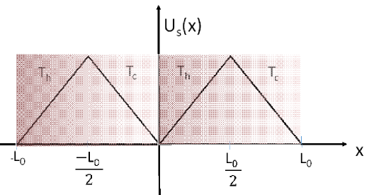
We consider a Brownian particle that moves along the potential $U(x)=U_{s}(x)+fx$ where $f$ and $U_{s}(x)$ denote the load and ratchet potential, respectively. The ratchet potential $U_{s}(x)$

$$U_{s}(x)=\left\{\begin{array}[]{cl}2U_{0}[{x\over L_{0}}],&if~{}0<x\leq L_{0}/2;\\ 2U_{0}[{-x\over L_{0}}+1],&if~{}L_{0}/2<x\leq L_{0};\end{array}\right.$$ (1)

is coupled with a heat bath that decreases from $T_{h}$ at $x=0$ to $T_{c}$ at $x=L_{0}$ along the reaction coordinate in the manner

$$T(x)=\left\{{x(T_{c}-T_{h})\over L_{0}}+T_{h}\right\}.$$ (2)

Here $U_{0}$ and $L_{0}$ denote the barrier height and the width of the ratchet potential, respectively. The ratchet potential has a potential maxima at $x=L_{0}/2$ and potential minima at $x=0$ and $x=L_{0}$. The potential profile repeats itself such that $U_{s}(x+L_{0})=U_{s}(x)$.

In the high friction limit, the dynamics of the particle is governed by the Langevin equation. The general stochastic Langevin equation which derived in the pioneering work of Petter Hänggi am1 ; am2 can be written as

$$\gamma(x){dx\over dt} = -{\partial U(x)\over\partial x}-{(1-\epsilon)\over\gamma(x)}{\partial\over\partial x}(\gamma(x)T(x))+$$

$$\sqrt{2k_{B}\gamma(x)T(x)}\xi(t)$$

following the approach stated in the work am3 . The Ito and Stratonovich interpretations correspond to the case where $\epsilon=1$ and $\epsilon=1/2$, respectively while the case $\epsilon=0$ is known as the Hänggi a post-point or transform-form interpretation. Here after we adapt the Langevin equation

$$\gamma(x){dx\over dt} = -{\partial U(x)\over\partial x}+\sqrt{2k_{B}\gamma(x)T(x)}\xi(t).$$ (4)

$\gamma(x)$ is the viscous friction, and $k_{B}$ is the Boltzmann’s constant. The random force $\xi(t)$ is considered to be Gaussian and white noise satisfying

$$\left\langle\xi(t)\right\rangle=0,~{}~{}~{}\left\langle\xi(t)\xi(t+\tau)\right\rangle=\delta(\tau).$$ (5)

The corresponding Fokker Planck equation is given by

$${\partial P(x,t)\over\partial t} = {\partial\over\partial x}({1\over\gamma}[U^{\prime}(x)P(x,t)+{\partial\over\partial x}(k_{B}T(x)P(x,t))])$$ (6)

$$= -{\partial J(x,t)\over\partial x}$$

where $P(x,t)$ is the probability density of finding the particle at position $x$ and time $t$, $J(x,t)$ denotes the current. Hereafter, the Boltzmann constant $k_{B}$ and $\gamma$ are taken to be unity.

We are interested in the long time behavior of the system. In this limit, the expression for the constant current, $J$, is given by

$${1\over\gamma}\left[-U^{\prime}(x)P^{s}(x)+{d\over dx}(T(x)P^{s}(x))\right]=J.$$ (7)

It is important to note that in the absence of symmetry breaking fields, no net flow of particles is obtained. Only in the presence of externally acting load or inhomogeneous temperature distribution, a unidirectional motion of particle is attainable. Hereafter, for sake of simplicity, we introduce dimensionless rescaled temperature $\tau=T_{h}/T_{c}$, rescaled barrier height ${\bar{U}_{0}}=U_{0}/T_{c}$ and rescaled length ${\bar{x}}=x/L_{0}$. Hereafter for simplicity the bar will be neglected.

The general expression for the steady state current $J$ in any periodic potential with or without load is reported in the works c9 ; c11 . Following the same approach, we find the steady state current J as

$$J={-F\over G_{1}G_{2}+HF}.$$ (8)

where the expressions for F, G1, G2, and H are given as

$$F = -1+e^{-\frac{2U_{2}\text{ln}\left[\frac{2}{1+\tau}\right]}{1-\tau}+\frac{2U_{1}\text{ln}\left[\frac{1+\tau}{2\tau}\right]}{1-\tau}},$$ (9)

$$G_{1} = \frac{1-4^{\frac{U_{1}}{1-\tau}}\left(\frac{\tau}{1+\tau}\right)^{\frac{2U_{1}}{1-\tau}}}{2U_{1}}+$$ (10)

$$\frac{2^{-1+\frac{2U_{1}}{1-\tau}}\left(\frac{1+\tau}{\tau}\right)^{-\frac{2U_{1}}{1-\tau}}\left(-1+4^{\frac{U_{2}}{1-\tau}}\left(\frac{1}{1+\tau}\right)^{\frac{2U_{2}}{1-\tau}}\right)}{U_{2}},$$

$$G_{2} = \frac{1}{2}\left(\frac{2\tau}{-1+\tau-2U_{1}}-\frac{4^{\frac{U_{1}}{-1+\tau}}\left(1+\frac{1}{\tau}\right)^{-\frac{2U_{1}}{-1+\tau}}(1+\tau)}{-1+\tau-2U_{1}}\right)+$$ (11)

$${1\over 2}\left(\frac{4^{\frac{U_{1}}{-1+\tau}}\left(1+\frac{1}{\tau}\right)^{-\frac{2U_{1}}{-1+\tau}}\left(1+\tau-2^{1+\frac{2U_{2}}{-1+\tau}}\left(\frac{1}{1+\tau}\right)^{\frac{2U_{2}}{-1+\tau}}\right)}{-1+\tau+2U_{2}}\right),$$

$$H = T_{1}+T_{2}(T_{3}+T_{4}+T_{5}),$$ (12)

$$T_{1} = \frac{\tau\left(-1+4^{\frac{U_{1}}{1-\tau}}\left(\frac{\tau}{1+\tau}\right)^{\frac{2U_{1}}{1-\tau}}\right)+U_{1}}{2U_{1}(1-\tau+2U_{1})},$$ (13)

$$T_{2} = 2^{-2+\frac{2(U_{1}+U_{2})}{1-\tau}}\left(\frac{1+\tau}{\tau}\right)^{-\frac{2U_{1}}{1-\tau}},$$ (14)

$$T_{3} = \frac{2^{\frac{1-\tau-2(U_{1}+U_{2})}{1-\tau}}\left(\frac{1+\tau}{\tau}\right)^{\frac{2U_{1}}{1-\tau}}}{1-\tau-2U_{2}}+\frac{2\tau\left(-4^{-\frac{U_{2}}{1-\tau}}+\left(\frac{1}{1+\tau}\right)^{\frac{2U_{2}}{1-\tau}}\right)}{(-1+\tau-2U_{1})U_{2}},$$ (15)

$$T_{4} = \frac{2^{-\frac{2U_{1}}{1-\tau}}(1+\tau)\left(\frac{1+\tau}{\tau}\right)^{\frac{2U_{1}}{1-\tau}}\left(-2^{-\frac{2U_{2}}{1-\tau}}+\left(\frac{1}{1+\tau}\right)^{\frac{2U_{2}}{1-\tau}}\right)}{(1-\tau+2U_{1})U_{2}},$$ (16)

$$T_{5} = -\frac{2^{-\frac{2U_{1}}{1-\tau}}(1+\tau)\left(\frac{1+\tau}{\tau}\right)^{\frac{2U_{1}}{1-\tau}}\left(-2^{-\frac{2U_{2}}{1-\tau}}+\left(\frac{1}{1+\tau}\right)^{\frac{2U_{2}}{1-\tau}}\right)}{(1-\tau-2U_{2})U_{2}}.$$ (17)

Here $U_{1}=U_{0}+f/2$ and $U_{2}=U_{0}-f/2$. The expression for the velocity is then given by $V=LJ$.

III The mobility of the particle

Figure 2: (Color online)(a) The velocity $V$ as a function of $U_{0}$ for the parameter value of $\tau=2.0$. The parameter $\lambda$ is fixed as $\lambda=0.5$, $\lambda=0.8$ and $\lambda=1.1$ from top to bottom, respectively. (b) The velocity $V$ as a function of $\lambda$ for the parameter value of $\tau=2.0$. The parameter $U_{0}$ fixed as $U_{0}=4.0$, $U_{0}=2.0$ and $U_{0}=1.0$ from top to bottom, respectively.

Figure 3: (Color online)(a) $V$ as a function of $\tau$ for the parameter value of $\lambda=1.0$. The parameter $U_{0}$ fixed as $U_{0}=4.0$, $U_{0}=2.0$ and $U_{0}=1.0$ from top to bottom, respectively. (b) $V$ as a function of $\tau$ for the parameter value of $U_{0}=2.0$. The parameter $\lambda$ fixed as $\lambda=0.0$, $\lambda=0.5$ and $\lambda=1.0$ from top to bottom, respectively.

Various studies on Brownian heat engine that operates on the reaction coordinate that coupled with a spatially varying temperature have depicted that the motor attains a unidirectional motion as long as a distinct temperature difference is retained along the potential. The dependence of the steady state current or the velocity on the barrier height $U_{0}$ can be explored by exploiting Eq. (8). One can see that in the absence of the ratchet potential, the average velocity of the particle is zero, i.e.; the velocity $V$ vanishes when $U_{0}\to 0$. In the limit $U\to\infty$, $V\to 0$ which is expected because in the high barrier limit, the particle encounters a difficulty of surmounting the high potential barrier. In the presence of a load, the engine exhibits an intriguing dynamics where the magnitude of the load dictates the direction of the particle flow. The steady state current is zero at stall load

$$f_{s}={2U_{0}\over L}{\ln\left[{4\tau\over(1+\tau)^{2}}\right]\over\ln\left[{1\over\tau}\right]}.$$ (18)

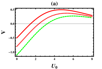
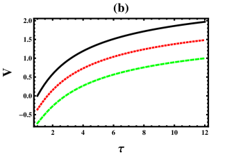
The velocity $V$ as a function of $U_{0}$ for the parameter value of $\tau=2.0$ is plotted in Fig. 2a for fixed $\lambda=0.5$, $\lambda=0.8$ and $\lambda=1.1$ from top to bottom, respectively. The figure depicts that the velocity steps up as $U_{0}$ increases and at a certain potential height, the velocity attains its maximum value and it decreases as the potential further increases. The velocity $V$ as a function of $\lambda$ for the parameter value of $\tau=2.0$, $U_{0}=4.0$, $U_{0}=2.0$ and $U_{0}=1.0$ is shown in Fig. 2b. when $f<f_{s}$, $V>0$ in this regime the model acts as a heat engine while $f>f_{s}$, $V<0$ in this case the model function as a refrigerator. The magnitude of the steady state current also strictly relies on the rescaled temperature $\tau$. When $\tau$ steps up, the tendency of the particle in the hotter bath to reach the top of the ratchet potential hill increases than the particle in the colder reservoir. This leads to an increase in the current $J$ or the drift velocity $V$ as shown in Figs. 3a and 3b. In Fig. 3a, we plot $V$ as a function of $\tau$ for the parameter value of $\lambda=1.0$. The parameter $U_{0}$ is fixed as $U_{0}=4.0$, $U_{0}=2.0$ and $U_{0}=1.0$ from top to bottom, respectively. The figure depicts that the velocity increases as $\tau$ and $U_{0}$ increase. The dependence for the velocity on $\tau$ is also explored in Fig. 3b for the parameter value of $U_{0}=2.0$. The parameter $\lambda$ is fixed as $\lambda=0.0$, $\lambda=0.5$ and $\lambda=1.0$ from top to bottom, respectively. The figure exhibits that the velocity increases with $\tau$ and it decreases as the load increases.

IV The performance of the motor

IV.1 Energetics of the motor

The expressions for the work done by the Brownian particle as well as the amount heat taken from the hot bath and the amount of heat given to the cold reservoir can be derived in terms of the stochastic energetics discussed in the works am4 ; am5 ; am6 . Let us first omit the heat dissipation via friction. The heat taken from any heat bath can be evaluated via am4 ; am5 ${\dot{Q}}=\left\langle\left(-\gamma(x){\dot{x}}+\sqrt{2k_{B}\gamma(x)T(x)}\right).{\dot{x}}\right\rangle$ while the work done by the Brownian particle against the load is given by ${\dot{W}}=\left\langle f{\dot{x}}\right\rangle.$ We can also find the expression for the input heat $Q_{in}^{s}$ and $W^{s}$ am6 as

$$Q_{in}^{s} = \int_{0}^{L_{0}/2}\left(-\gamma(x){\dot{x}}+\sqrt{2k_{B}\gamma(x)T(x)}\right)dx$$

$$= \int_{0}^{L_{0}/2}\left[\left({2U_{0}\over L_{0}}\right)+f\right]dx$$

$$= U_{0}+{fL_{0}\over 2}.$$

Here the integral is evaluated in the interval of $(0,L_{0}/2)$ since the particle has to get a minimal amount of heat input from the heat bath located in the left side of the ratchet potential to surmount the potential barrier. The work done is also given by

$$W^{s} = \int_{0}^{L_{0}}fdx=fL_{0}.$$ (20)

The first law of thermodynamics states that $Q_{in}^{s}-Q_{out}^{s}=W^{s}$ where $Q_{out}^{s}$ is the heat given to the colder heat bath. Thus $Q_{out}^{s}=Q_{in}^{s}-W^{s}=U_{0}-{fL_{0}\over 2}.$

If one includes the heat dissipation via the viscous friction, the minimum heat dissipation occurs when the motor hops with a constant velocity ${\dot{x}}=V$ c14 . In this case, an extra amount of heat $Q_{in}^{*}$ has to be taken from the hotter bath to overcome the friction. The average work done against the viscous friction is given by

$$W^{*} = \int_{0}^{L_{0}}\gamma(x){\dot{x}}dx$$

$$= \gamma({VL_{0}})=\gamma({JL_{0}^{2}})$$

$$= F_{av}L_{0}$$

where the average force $F_{av}=\gamma({JL_{0}})$. On the other hand on average the heat taken from the hotter bath to overcome the frictional force is given as

$$Q_{in}^{*} = \int_{0}^{L_{0}/2}F_{av}dx$$

$$= \gamma({VL_{0}\over 2})=\gamma({JL_{0}^{2}\over 2}).$$

Since $Q_{in}^{*}-Q_{out}^{*}=W^{*}$ and one finds

$$Q_{out}^{*} = Q_{in}^{*}-W^{*}=-\gamma({JL_{0}^{2}\over 2}).$$ (23)

In addition, ${1\over 2}{k_{B}(T_{h}-T_{c})}$ amount of heat per cycle is transferred from the hotter to the colder heat baths via the kinetic energy in one cycle. Thus for single Brownian particle crossing over the potential barrier, the amount of heat energy taken from the hot reservoir in one cycle is given by $Q_{in}=Q_{in}^{s}+Q_{in}^{*}+{1\over 2}k_{B}(T_{h}-T_{c})=\left(U_{0}+\gamma J{L_{0}^{2}\over 2}+f{L_{0}\over 2}+{1\over 2}k_{B}(T_{h}-T_{c})\right).$ This does make sense since in one cycle, a minimum $(U_{0}+\gamma J{L_{0}^{2}\over 2}+f{L_{0}\over 2})$ amount of heat is needed to overcome the viscous drag force $\gamma V/2$, the potential barrier $U_{0}$ and the external load $f$. In addition, ${1\over 2}{k_{B}(T_{h}-T_{c})}$ amount of heat per cycle is transferred from the hotter to the colder heat baths. The heat given to the cold reservoir takes a form $Q_{out}=Q_{out}^{s}+Q_{out}^{*}+{1\over 2}k_{B}(T_{h}-T_{c})=\left(U_{0}-\gamma J{L_{0}^{2}\over 2}-f{L_{0}\over 2}+{1\over 2}k_{B}(T_{h}-T_{c})\right).$ The work done against the load and the viscous friction is given by $W=Q_{in}-Q_{out}=W^{s}+W^{*}=\gamma({JL_{0}^{2}})+fL_{0}.$ If the motor acts as a refrigerator, the net heat flow to the cold heat bath is given by c10 $Q_{c}=\left(U_{0}-\gamma J{L_{0}^{2}\over 2}-f{L_{0}\over 2}-{1\over 2}k_{B}(T_{h}-T_{c})\right).$ Moreover the efficiency is given as

$$\eta=W/Q_{in}.$$ (24)

The performance of the refrigerator is also given by

$$P_{ref}=Q_{out}/W^{L}$$ (25)

where $W^{L}=fL_{0}$.

IV.2 The efficiency of the heat engine

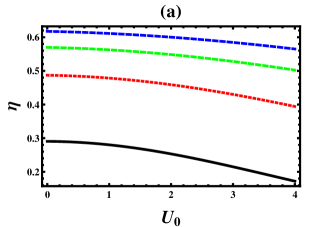
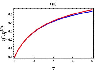
The heat exchange via the potential.— We now explore the dependence of the efficiency $\eta$ on the model parameters. To start with we first look at how $\eta$ depends on the barrier height and the rescaled temperature $\tau$ by omitting the heat exchange via kinetic energy. The efficiency $\eta$ as a function of $U_{0}$ is depicted in Fig. 4a for the parameter values of $\lambda=0.0$, $\tau=8.0$, $\tau=6.0$, $\tau=4.0$ and $\tau=2.0$ from top to bottom, respectively. The figure exhibits that $\eta$ decreases from its maximum (quasistatic ) value as $U_{0}$ and $\tau$ increases. In the quasistatic limit $U_{0}\to 0$ ($J\to 0$), we find

$$\eta^{*}=1-{ln\left[{1+\tau\over 2\tau}\right]\over ln\left[{2\over\tau+1}\right]}$$ (26)

which is approximately equal to the efficiency of the endorevesible heat engine $\eta_{CA}$

$$\eta_{CA}=1-\sqrt{1/\tau}$$ (27)

as long as the temperature difference between the hot and the cold reservoirs is not large. In order to appreciate this let us Taylor expand Eqs. (26) and (27) around $\tau=1$ and after some algebra one gets

$$\eta^{*} = \eta_{CA}={\tau-1\over 2}-{3\over 8}(\tau-1)^{2}+\ldots$$ (28)

$$= {\eta_{CAR}\over 2}+{\eta_{CAR}^{2}\over 8}+{\eta_{CAR}^{3}\over 96}+\ldots$$

which exhibits that both efficiencies are equivalent in this regime. Here $\eta_{CAR}$ is the Carnot efficiency $\eta_{CAR}=1-\sqrt{1/\tau}$. As discussed in the work mu25 , it is still unknown why different model systems approach the Taylor expression shown above. Indeed $\eta_{C}$ and $\eta_{CA}$ still precisely agree even at higher temperature difference as shown in Fig. 6a.

The efficiency $\eta$ as a function of $U_{0}$ is plotted in Fig. 4a for the parameter values of $\lambda=0.0$, $\tau=8.0$, $\tau=6.0$, $\tau=4.0$ and $\tau=2.0$. The efficiency decreases as the barrier height increases. When the magnitude of the rescaled temperature steps up, the efficiency of the motor monotonously increases. The dependence of $\eta$ on the rescaled temperature $\tau$ is depicted in Fig. 4b for the parameter values of $\lambda=0.0$, $U_{0}=1.0$, $U_{0}=2.0$, $U_{0}=4.0$ and $U_{0}=8.0$. The figure exhibits that the efficiency steps up with $\tau$ and it decreases as the barrier height decreases.

Figure 4: (Color online)(a) The efficiency $\eta$ as a function of $U_{0}$ for the parameter values of $\lambda=0.0$, $\tau=8.0$, $\tau=6.0$, $\tau=4.0$ and $\tau=2.0$ from top to bottom, respectively. (b) $\eta$ as a function of $\tau$ for the parameter values of $\lambda=0.0$, $U_{0}=1.0$, $U_{0}=2.0$, $U_{0}=4.0$ and $U_{0}=8.0$ from top to bottom, respectively.

In the presence of load, the quasistatic limit of the engine corresponds to the case where the current approaches zero either from the heat engine side or from the refrigerator. The steady state current is zero at stall load (see Eq. 18). This stall force serves as a boundary that demarcating the domain of operation of the engine. When $f<f_{s}$ the model acts as a heat engine while as long as $f>f_{s}$ the model behaves as refrigerator. In quasistatic limit $J\to 0$, once again we find $\eta_{CA}\approx\eta_{C}=1-{ln\left[{1+\tau\over 2\tau}\right]\over ln\left[{2\over\tau+1}\right]}$.

Figure 5: (Color online)(a) The efficiency $\eta$ as a function of $U_{0}$ that plotted by considering the heat exchange via the kinetic energy. The parameters are fixed as $\lambda=0.0$, $\tau=4.0$ and $\tau=2.0$ from top to bottom, respectively. (b) $\eta$ as a function of $\tau$ for the parameter values of $\lambda=0.0$, $U_{0}=2.0$ and $U_{0}=6.0$ from top to bottom, respectively.

The heat exchange via kinetic energy .— Let us now examine the thermodynamic property of the engine by including the heat exchange via the kinetic energy. When the heat exchange via the kinetic energy is included Carnot efficiency will not be obtained even at the quasistatic limit. This is due to the fact that the heat flow via kinetic energy is irreversible.

The dependence of the efficiency on the model parameters is also examined by including the heat exchange via kinetic energy. At quasistatic limit, the steady state efficiency takes a form

$$\eta={\eta^{*}\over\Omega}$$ (29)

where $\Omega$ is given by

$$\Omega=\tau+{((-1+\tau)Log[\tau])\over(Log[4]-2Log[1+\tau])}$$ (30)

Here $0<{1\over\Omega}<1$, revealing that the efficiency can never approaches the quasistatic efficiency $\eta^{*}$ that evaluated by omitting the heat exchange via kinetic energy.

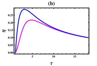
The dependence of $\eta$ on the barrier height is explored in Fig. 5a. In the figure, the parameters are fixed as $\lambda=0.0$, $\tau=4.0$ and $\tau=2.0$ from top to bottom, respectively. The figure depicts that the efficiency decreases as the barrier height $U_{0}$ decreases. As shown in the same figure, the efficiency decreases as $\tau$ decreases. In Fig. 5b, we plot $\eta$ as a function of $\tau$ for the parameter values of $\lambda=0.0$, $U_{0}=2.0$ and $U_{0}=6.0$ from top to bottom, respectively. The same figure depicts that $\eta=0$ when $\tau=1$ and it increases with $\tau$. The efficiency attains an optimal value at a certain $\tau$ and it then decreases as $\tau$ further increases. $\eta$ also decreases as $U_{0}$ increases.

IV.3 Optimal and maximum power efficiency

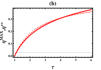
The efficiency of the engine at maximum power $\eta^{MAX}$ is analyzed by substituting the values of $U_{0}$ and $\tau$ at which $J$ is maximum. Fig. 6b (dotted line) depicts $\eta^{MAX}$ as a function of $\tau$ for fixed $U_{0}=2$. As it can be seen clearly $\eta^{MAX}$ is approximately the same as the efficiency

$$\eta^{**}=1-(1/\tau)^{(}1/4)$$ (31)

at least in the small $\tau$ region. In fact $\eta^{MAX}$ and $\eta^{**}$ still precisely agree even at higher temperature difference as shown in Fig. 6b.

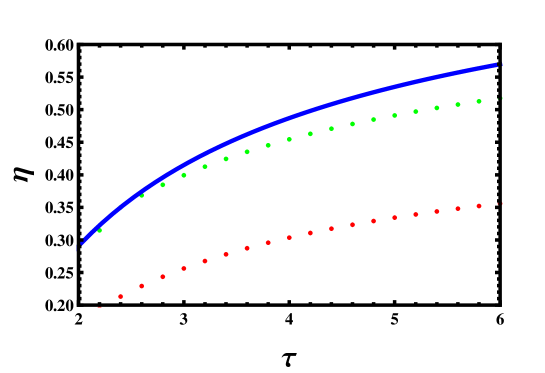
On the other hand, the optimized efficiency (OPT) is the efficiency where the competition between energy cost and fast transport is compromised c9 . Following the same approach as the work c9 ; cc20 , we optimize the function $\Omega=2W-{\tau-1\over\tau}Q_{in}$. In Fig. 7, we plot the optimal efficiency as a function of $\tau$ (see the intermediate line). We want to stress that when the engine operates at quasistatic limit, the efficiency approaches $\eta^{*}$ (see the top line of Figs. 7) which is the maximum possible efficiency. At this operation regime, the particle velocity is zero (zero energy cost). On the other hand, when the engine operates at maximum power, the velocity of the motor is maximum implies that the energy cost is higher and as a result, it becomes less efficient. However, the optimal efficiency (green dotted line) lies between $\eta^{8}$ and maximum power efficiency (red dotted line) as it can be seen in Fig. 7.

The main message here is that by selecting proper parameter space, we can control the operation as well as its task. The operation regime at quasistatic limit is the least desirable one since one should wait an infinite time for the engine to accomplish its task although the efficiency at this operation regime is the maximum one; in other words, the system delivers a zero power. If one needs a motor that moves fast along the reaction coordinate, a proper value of $U_{0}$ that maximize the velocity can be selected as a possible model ingredient. A compromised effect can be seen at optimal power efficiency regime.

Figure 6: (Color online)(a) The quasistatic efficiency $\eta^{*}$ (red line) and the efficiency $\eta^{CA}$ (blue line) as a function of $\tau$. (b) The maximum efficiency $\eta^{MAX}$ (dotted line) and $\eta^{**}$ (solid line) as a function of $\tau$.

Figure 7: The efficiency $\eta$ as a function of $\tau$ for the parameter values of $\lambda=0.5$ and $U_{0}=8.0$. In the figure the top line stands for quasistatic efficiency $\eta^{*}$, the intermediate and the bottom line stand for optimum (OPT) and maximum power (MP) efficiencies, respectively.

Figure 8: (Color online)(a) The $P_{ref}$ as a function of $\lambda$. (b) The $P_{ref}$ as a function of $\lambda$ plotted considering the heat exchange via the kinetic energy. In both figures the parameters are fixed as $U_{0}$ and $\tau=6.0$

Figure 9: (Color online)(a) Phase diagram in $\tau$ and $U_{0}$ space for a given $\lambda=2.0$. (b) Phase diagram in $\tau$ and $\lambda$ space for a given $U_{0}=2.0$.

IV.4 Coefficient of performance of the refrigerator

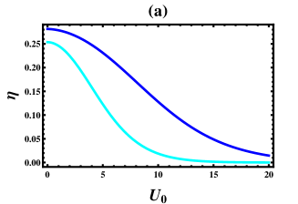
The coefficient performance of the refrigerator $P_{ref}$ is also explored as a function of the determinant model parameters. At quasistatic limit, $P_{ref}$ always approaches

$$P_{ref}^{*}={\ln\left[{1\over 2}\left[{1\over\tau}+1\right]\right]\over\ln\left[{4\tau\over(1+\tau)^{2}}\right]}$$ (32)

which is much less than Carnot refrigerator. As it can be readily seen that $P_{ref}^{*}$ decreases as $\tau$ increases.

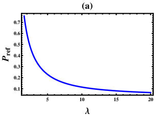
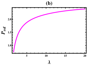
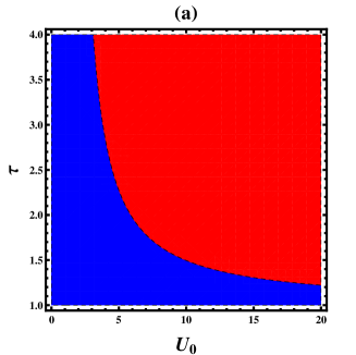
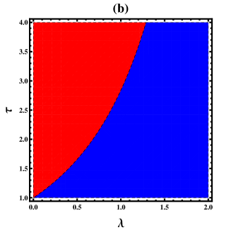
The plot for $P_{ref}$ as a function of $\lambda$ is depicted in Fig. 8a for fixed $U_{0}=2.0$ and $\tau=6.0$. $P_{ref}$ decreases as the load increases. The heat exchange between the heat baths via the kinetic energy has also influence on $P_{ref}$. Figure 8b shows that the coefficient of performance of the refrigerator increases as the load increases. Omitting the heat exchange via the kinetic energy, a complete picture for the operation regions of the heat engine is obtained by plotting the phase diagram in parameter space of $\tau$ and $U_{0}$ as shown in Fig. 9a. On the other hand, the phase diagram in parameter space of $\tau$ and $\lambda$ is plotted in Fig. 9b. In both figures, the region that marked red, the model works as a heat engine while in the region that marked in blue the model acts as a refrigerator.

V Short time case

In this work, we study the thermodynamic features of the engine via numerical simulations. The numerical results reveal the sensitivity of the performance of the thermal engine to the time $t$. The operation regimes of the engine are dictated by the operation time $t$. In the early particle relaxation period (small $t$), the engine neither acts as a heat engine nor as a refrigerator. This is because, when the system relaxation time is less than the time that the engine needs to perform work, the energy taken from the hot bath dissipates without doing any work. When $t$ further increases, depending on the parameter choice, the motor may work as a heat engine or as a refrigerator. Its performance is also an increasing function of $t$. Furthermore the engine depicts a higher efficiency or performance as a refrigerator at steady state regime. Moreover, we show that, when one omits the heat exchange via the kinetic energy, Carnot refrigerator and Carnot efficiency are unattainable even when the system operates quasistatically at the steady state regime. The magnitude and the direction of the velocity are also controlled by $t$.

Figure 10: (Color online)(a) The velocity $V$ as a function of $t$ for parameter choice of $U_{0}=3.0$, $\lambda=0.2$. The rescaled temperature is fixed as $\tau=8.0$ and $\tau=2.0$ from top to bottom. (b) The efficiency $\eta$ as a function of $t$ for parameter choice of $U_{0}=3.0$ and $\lambda=0.2$. The rescaled temperature is fixed as $\tau=8.0$, $\tau=6.0$, $\tau=4.0$ and $\tau=2.0$ from top to bottom.

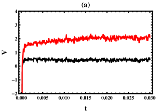
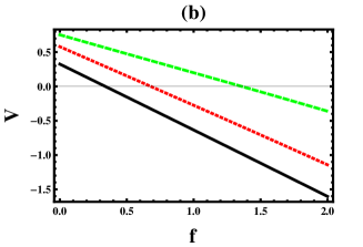
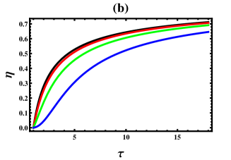
The short time behavior of the velocity is quite sensitive to time $t$. In this case the magnitude and the direction of the velocity are dictated by $t$. This can be notably appreciated by looking at Fig. 10a. The figure depicts that, for very small $t$, the net particle flow is from the colder to the hotter regions. As time increases,the magnitude of $V$ increases and stalls at certain time $t$. As time further steps up, the particle current gets reversed and the particle moves from the hotter to the colder reservoirs until its velocity saturates to a constant value. The results obtained in this work also agrees with our previous work c19 . The exact analytical work shown in the work c19 also uncovers current reversal due to time $t$. The efficiency $\eta$ as a function of time is also shown in Fig. 10b for parameter choice of $U_{0}=3.0$ and $\lambda=0.2$. The rescaled temperature is fixed as $\tau=8.0$, $\tau=6.0$, $\tau=4.0$ and $\tau=2.0$ from top to bottom. One can see that $\eta\ll\eta^{*}$ this is because the model is operating at finite time and also $\lambda=0.2\ll f_{s}$. The same figure depicts that the efficiency steps up with time. As the rescaled temperature increases, the efficiency increases as expected.

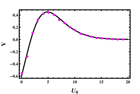
Our numerical results depict that for large time $t$ (approaching steady state), the velocity (see Fig. 11) as well as the efficiency approach their steady state value. In Fig. 11, we plot $V$ as a function of $U_{0}$ for a given rescaled $t=100$, $\lambda=0.6$ and $\tau=2$. The numerically evaluated velocity (dotted line) coincides with the velocity evaluated via Eq. (18) (exact expression). Moreover, our analysis indicates that the coefficient of performance of the heat refrigerator improves with time. At large $t$ (steady state), the velocity, efficiency and coefficient of performance of the refrigerator attain their maximum value.

Figure 11: The efficiency $\eta$ as a function of $U_{0}$ for the parameter values of $\lambda=0.6$, $t=100.0$ and $\tau=2.0$. The numerically evaluated velocity (dotted line) coincides with the velocity evaluated via Eq. (18) (solid line).

VI Summary and conclusion

In this work, we consider a Brownian heat engine that modeled as a particle hopping in a one-dimensional periodic ratchet potential that coupled with a linearly decreasing background temperature. Extending the previous work c17 , we uncover far more results. The dependence of the velocity, the efficiency and performance of the refrigerator on the model parameters is explored a by excluding the heat exchange via the kinetic energy. We show that the efficiency of such Brownian heat engine is far from Carnot efficiency even at quaistatic limit. At quasistatic limit, the efficiency of the heat engine approaches the efficiency of endoreversible engine $\eta=1-\sqrt{{T_{c}/T_{h}}}$ c18 . On the other hand, the maximum power efficiency of the engine approaches $\eta^{MAX}=1-({T_{c}/T_{h}})^{1\over 4}$. It is shown that the optimized efficiency always lies between the efficiently at quaistatic limit and the efficiency at maximum power. The efficiency at maximum power is always less than the optimized efficiency since the fast motion of the particle comes at the expense of the energy cost. If one includes the heat exchange at the boundary of the heat baths, the efficiency as well as the coefficient performance of the engine becomes much smaller than the Carnot efficiency or refrigerator. The dependence for the coefficient of performance of the refrigerator on the model parameters is also explored.

Via numerical simulations, we study the role of time on the performance of the motor. The numerical results show that the velocity of the particle increases with time. The external load detects the direction of the particle velocity. When the load is small, the net particle flow is towards the right direction and the model may act as a heat engine. For large load, current reversal occurs and the engine may work as a refrigerator. The efficiency of the engine explicitly relies on time. As time increases, the efficiency increases. At steady state, it saturates to a constant value. At small time $t$, the efficiency is much less than Carnot efficiency showing that the system exhibits irreversibility at small $t$. The coefficient of performance of the refrigerator also steps up as time increases. As $t$ further steps up, it converges to a constant value.

In conclusion, the model of Brownian heat engine which is presented in this work serves as a guide in the construction of artificial microscopic heat engine and also it is crucial for fundamental understanding of the nonequilibrium physics. We also believe that the present study serves as a basic exemplar to study the transport feature of biologically relevant systems such as polymers and membranes.

References

- (1) P. Hänggi, F. Marchesoni, and F. Nori, Ann. Phys. (Leipzig) 14, 51 (2005).
- (2) P. Hänggi and F. Marchesoni, Rev. Mod. Phys. 81, 387 (2009).
- (3) T. Hondou and K. Sekimoto, Phys. Rev. E 62, 6021 (2000).
- (4) A.G. Marin and J.M. Sancho, Phys. Rev. E 74, 062102 (2006).
- (5) N. Li, F. Zhan, P. Hänggi, and B. Li, Phys. Rev. E 80, 011125 (2009).
- (6) N. Li, P. Hänggi, and B. Li, Europhysics Letters 84, 40009 (2008).
- (7) F. Zhan, N. Li, S. Kohler, and P. Hänggi, Phys. Rev. E 80, 061115 (2009).
- (8) M. Büttiker, Z. Phys. B 68, 161 (1987).
- (9) N.G. van Kampen, IBM J. Res. Dev. 32, 107 (1988).
- (10) R. Landauer, J. Stat. Phys. 53, 233 (1988).
- (11) R. Landauer, Phys. Rev. A 12, 636 (1975).
- (12) R. Landauer, Helv. Phys. Acta 56, 847 (1983).
- (13) P. Reimann, R. Bartussek, R. Häussler, and P. Hänggi, Phys. Lett. A 215, 26 (1996).
- (14) M. Asfaw and M. Bekele, Eur. Phys. J. B 38, 457 (2004).
- (15) M. Asfaw and M. Bekele, Phys. Rev. E 72, 056109 (2005).
- (16) M. Asfaw and M. Bekele, Physica A 384, 346 (2007).
- (17) M. Matsuo and S. Sasa, Physica A 276, 188 (1999).
- (18) I. Derènyi and R.D. Astumian, Phys. Rev. E 59, R6219 (1999).
- (19) I. Derènyi, M. Bier, and R.D. Astumian, Phys. Rev. Lett 83, 903 (1999).
- (20) J.M. Sancho, M. S. Miguel, and D. Dürr, J. Stat. Phys. 28, 291 (1982).
- (21) B.Q. Ai, H.Z. Xie, D.H. Wen, X.M. Liu, and L.G. Liu, Eur. Phys. J. B 48, 101 (2005).
- (22) M. Asfaw, Eur. Phys. J. B 86, 189 (2013).
- (23) F. L. Curzon and B. Ahlborn, Am. J. Phys. 43, 22 (1975).
- (24) M. Asfaw, Phys. Rev. E 89, 012143 (2014).
- (25) O. Reynolds, Phil Trans Royal Soc London 177, 157 ((1886).
- (26) M. Asfaw and S. F. Duki, Eur. Phys. J. B 88, 322 (2015).
- (27) P. Hänggi, Helv. Phys. Acta 51, 183 (1978).
- (28) P. Hänggi, Helv. Phys. Acta 53, 491 (1980).
- (29) J. M. Sancho, M. S. Miguel and D. Duerr, J. Stat. Phys. 28, 291 (1982).
- (30) K. Sekimoto, J. Phys. Soc. Jpn. 66, 1234 (1997).
- (31) K. Sekimoto, Prog. Theor. Phys. Suppl. 130, 17 (1998).
- (32) M. Matsuo, , Shin-ichi Sasa, Physica A 276, 188 (2000).
- (33) A. Calvo Hernandez, J. M. M. Roco, and A. Medina, Revista Mexicana de Fısica 60, 384 (2014).