Abstract

For the search for additional Higgs bosons in the Minimal Supersymmetric Standard Model (MSSM) as well as for future precision analyses in the Higgs sector precise knowledge of their production properties is mandatory. We evaluate the cross sections for the charged Higgs boson production at $e^{+}e^{-}$ colliders in the MSSM with complex parameters (cMSSM). The evaluation is based on a full one-loop calculation of the production mechanism $e^{+}e^{-}\to H^{+}H^{-}$ and $e^{+}e^{-}\to H^{\pm}W^{\mp}$, including soft and hard QED radiation. The dependence of the Higgs boson production cross sections on the relevant cMSSM parameters is analyzed numerically. We find sizable contributions to many cross sections. They are, depending on the production channel, roughly of 5–10% of the tree-level results, but can go up to 20% or higher. the full one-loop contributions are important for a future linear $e^{+}e^{-}$ collider such as the ILC or CLIC.

1 Introduction

The identification of the underlying physics of the Higgs boson discovered at $\sim 125\,\,\mathrm{GeV}$ [1, 2] and the exploration of the mechanism of electroweak symmetry breaking will clearly be a top priority in the future program of particle physics. The most frequently studied realizations are the Higgs mechanism within the Standard Model (SM) [3] and within the Minimal Supersymmetric Standard Model (MSSM) [4, 5, 6]. Contrary to the case of the SM, in the MSSM two Higgs doublets are required. This results in five physical Higgs bosons instead of the single Higgs boson in the SM. In lowest order these are the light and heavy ${\cal CP}$-even Higgs bosons, $h$ and $H$, the ${\cal CP}$-odd Higgs boson, $A$, and two charged Higgs bosons, $H^{\pm}$. Within the MSSM with complex parameters (cMSSM), taking higher-order corrections into account, the three neutral Higgs bosons mix and result in the states $h_{i}$ ($i=1,2,3$) [7, 8, 9, 10]. The Higgs sector of the cMSSM is described at the tree level by two parameters: the mass of the charged Higgs boson, $M_{H^{\pm}}$, and the ratio of the two vacuum expectation values, $\tan\beta\equiv t_{\beta}=v_{2}/v_{1}$. Often the lightest Higgs boson, $h_{1}$ is identified [11] with the particle discovered at the LHC [1, 2] with a mass around $\sim 125\,\,\mathrm{GeV}$ [12]. If the mass of the charged Higgs boson is assumed to be larger than $\sim 200\,\,\mathrm{GeV}$ the four additional Higgs bosons are roughly mass degenerate, $M_{H^{\pm}}\approx m_{h_{2}}\approx m_{h_{3}}$ and referred to as the “heavy Higgs bosons”. Discovering one or more of the additional Higgs bosons would be an unambiguous sign of physics beyond the SM and could yield important information as regards their possible supersymmetric origin.

If supersymmetry (SUSY) is realized in nature and the charged Higgs boson mass is $M_{H^{\pm}}\lesssim 1.5\,\,\mathrm{TeV}$, then the additional Higgs bosons could be detectable at the LHC [13, 14] (including its high luminosity upgrade, HL-LHC; see Ref. [15] and references therein). This would yield some initial data on the extended Higgs sector. Equally important, the additional Higgs bosons could also be produced at a future linear $e^{+}e^{-}$ collider such as the ILC [16, 17, 18, 19] or CLIC [20, 19]. (Results on the combination of LHC and ILC results can be found in Ref. [21].) At an $e^{+}e^{-}$ linear collider several production modes for the cMSSM Higgs bosons are possible,

$$e^{+}e^{-} \to h_{i}Z,\,h_{i}\gamma,\,h_{i}h_{j},\,h_{i}\nu\bar{\nu},\,h_{i}e^{+}e^{-},\,h_{i}t\bar{t},\,h_{i}b\bar{b},\,\ldots\quad(i,j=1,2,3)\,,$$

$$e^{+}e^{-} \to H^{+}H^{-},\,H^{\pm}W^{\mp},\,H^{\pm}e^{\mp}\nu,\,H^{\pm}tb,\,\ldots\,.$$

In the case of a discovery of additional Higgs bosons a subsequent precision measurement of their properties will be crucial to determine their nature and the underlying (SUSY) parameters. In order to yield a sufficient accuracy, one-loop corrections to the various Higgs boson production and decay modes have to be considered. Full one-loop calculations in the cMSSM for various Higgs boson decays to SM fermions, scalar fermions and charginos/neutralinos have been presented over the last years [22, 23, 24]. For the decay to SM fermions see also Refs. [25, 26, 27]. Decays to (lighter) Higgs bosons have been evaluated at the full one-loop level in the cMSSM in Ref. [22]; see also Refs. [28, 29]. Decays to SM gauge bosons (see also Ref. [30]) can be evaluated to a very high precision using the full SM one-loop result [31] combined with the appropriate effective couplings [32]. The full one-loop corrections in the cMSSM listed here together with resummed SUSY corrections have been implemented into the code FeynHiggs [33, 34, 35, 32, 36]. Corrections at and beyond the one-loop level in the MSSM with real parameters (rMSSM) are implemented into the code HDECAY [37, 38]. Both codes were combined by the LHC Higgs Cross Section Working Group to obtain the most precise evaluation for rMSSM Higgs boson decays to SM particles and decays to lighter Higgs bosons [39].

The most advanced SUSY Higgs boson production calculations at the LHC are available via the code SusHi [40], which are, however, so far restricted to the rMSSM [41]. On the other hand, also particularly relevant are higher-order corrections also for the Higgs boson production at $e^{+}e^{-}$ colliders, where a very high accuracy in the Higgs property determination is anticipated [19]. A full one-loop calculation in the cMSSM of all neutral Higgs boson production channels with two final state particles, $e^{+}e^{-}\to h_{i}Z,h_{i}\gamma,h_{i}h_{j}$ ($i,j=1,2,3$) has recently been presented in Ref. [42]. There it was found that the one-loop corrections can change the tree-level result by roughly 10-20%, but can go up to 50% or higher. This motivates the evaluation of further Higgs boson production channels at the full one-loop level. Consequently, in this paper we take the next step and concentrate on the charged Higgs boson production at $e^{+}e^{-}$ colliders in association with a $W$ boson or second charged Higgs boson, i.e. we calculate,

$$\sigma(e^{+}e^{-}\to H^{+}H^{-})\,,$$ (1)

$$\sigma(e^{+}e^{-}\to H^{\pm}W^{\mp})\,.$$ (2)

The process $e^{+}e^{-}\to H^{\pm}W^{\mp}$ is loop-induced if the electron mass is neglected. Our evaluation of the two channels (1) and (2) is based on a full one-loop calculation, i.e. including electroweak (EW) corrections, as well as soft and hard QED radiation.

Results for the cross sections (1) and (2) at various levels of sophistication have been obtained over the last two decades. First loop corrections to the $H^{+}H^{-}$ production in the rMSSM, including third generation (s)fermion contributions were published in Refs. [43] and with (s)top/(s)bottom contributions in Ref. [44]. Loop corrections to $e^{+}e^{-}\to H^{+}H^{-}$ in the rMSSM, but restricted to the Two Higgs Doublet Model (THDM) contributions, were presented in Ref. [45]. Full one-loop calculations for $e^{+}e^{-}\to H^{+}H^{-}$ in the rMSSM were published in Ref. [46]. Similarly, loop corrections to $H^{\pm}W^{\mp}$ production in the rMSSM, but restricted to the THDM contributions, were presented in Refs. [47, 48, 49]. First full one-loop calculations for $e^{+}e^{-}\to H^{+}H^{-}$ and $e^{+}e^{-}\to H^{\pm}W^{\mp}$ in the rMSSM were published in Ref. [50] and Ref. [51], respectively. The effect of Sudakov logarithms on channel (1) were analyzed in Ref. [52]. Triple Higgs boson production at the one-loop level in the context of the THDM was published in Ref. [53], including a tree level calculation of channel (1). More phenomenological analyses on channel (2) were given in Ref. [54] and finally in Ref. [55], the latter relying on an independent re-evaluation in the rMSSM and the THDM. To our knowledge no calculation of $e^{+}e^{-}\to H^{+}H^{-},H^{\pm}W^{\mp}$ in the cMSSM has been performed so far. A numerical comparison with the literature will be given in Sect. 3.

In this paper we present for the first time a full and consistent one-loop calculation for charged cMSSM Higgs boson production at $e^{+}e^{-}$ colliders in association with a $W$ boson or a second charged Higgs boson. We take into account soft and hard QED radiation and the treatment of collinear divergences. In this way we go substantially beyond the existing calculations (see above). In Sect. 2 we very briefly review the renormalization of the relevant sectors of the cMSSM and give details as regards the calculation. In Sect. 3 various comparisons with results from other groups are given. the numerical results for the production channels (1) and (2) are presented in Sect. 4. The conclusions can be found in Sect. 5.

Prolegomena

We use the following short-hands in this paper:

• FeynTools $\equiv$ FeynArts + FormCalc + LoopTools.

• $s_{\mathrm{w}}\equiv\sin\theta_{W}$, $c_{\mathrm{w}}\equiv\cos\theta_{W}$.

• $t_{\beta}\equiv\tan\beta$.

They will be further explained in the text below.

2 Calculation of diagrams

In this section we give some details regarding the renormalization procedure and the calculation of the tree-level and higher-order corrections to the production of charged Higgs bosons in $e^{+}e^{-}$ collisions. The diagrams and corresponding amplitudes have been obtained with FeynArts (version 3.9) [56], using the MSSM model file (including the MSSM counterterms) of Ref. [57]. The further evaluation has been performed with FormCalc (version 9.3) and LoopTools (version 2.13) [58].

2.1 The complex MSSM

The cross sections (1) and (2) are calculated at the one-loop level, including soft and hard QED radiation; see the next section. This requires the simultaneous renormalization of the Higgs- and gauge-boson sector as well as the fermion sector of the cMSSM. We give a few relevant details as regards these sectors and their renormalization. More information can be found in Refs. [23, 24, 57, 59, 60, 61, 62, 63, 64, 65].

The renormalization of the fermion, Higgs and gauge-boson sector follows strictly Ref. [57] and references therein (see especially Ref. [32]). This defines in particular the counterterm $\delta t_{\beta}$, as well as the counterterms for the $Z$ boson mass, $\delta M_{Z}^{2}$, and for the sine of the weak mixing angle, $\delta s_{\mathrm{w}}$ (with $s_{\mathrm{w}}=\sqrt{1-c_{\mathrm{w}}^{2}}=\sqrt{1-M_{W}^{2}/M_{Z}^{2}}$, where $M_{W}$ and $M_{Z}$ denote the $W$ and $Z$ boson masses, respectively).

2.2 Contributing diagrams

Figure 1: Generic tree, self-energy, vertex, box, and counterterm diagrams for the process $e^{+}e^{-}\to H^{+}H^{-}$. $F$ can be a SM fermion, chargino or neutralino; $S$ can be a sfermion or a Higgs/Goldstone boson; $V$ can be a $\gamma$, $Z$ or $W^{\pm}$. It should be noted that electron–Higgs couplings are neglected.

Figure 2: Generic vertex, box, and counterterm diagrams for the (loop induced) process $e^{+}e^{-}\to H^{\pm}W^{\mp}$. $F$ can be a SM fermion, chargino or neutralino; $S$ can be a sfermion or a Higgs/Goldstone boson; $V$ can be a $\gamma$, $Z$ or $W^{\pm}$. It should be noted that electron–Higgs couplings are neglected.

Sample diagrams for the process $e^{+}e^{-}\to H^{+}H^{-}$ are shown in Fig. 1 and for the process $e^{+}e^{-}\to H^{\pm}W^{\mp}$ in Fig. 2. Not shown are the diagrams for real (hard and soft) photon radiation. They are obtained from the corresponding tree-level diagrams (i.e. only for channel (1)) by attaching a photon to the electrons/positrons and charged Higgs bosons. The internal particles in the generically depicted diagrams in Figs. 1 and 2 are labeled as follows: $F$ can be a SM fermion $f$, chargino $\tilde{\chi}_{c}^{\pm}$ or neutralino $\tilde{\chi}_{n}^{0}$; $S$ can be a sfermion ${\tilde{f}}_{s}$ or a Higgs (Goldstone) boson $h^{0},H^{0},A^{0},H^{\pm}$ ($G,G^{\pm}$); $U$ denotes the ghosts $u_{V}$; $V$ can be a photon $\gamma$ or a massive SM gauge boson, $Z$ or $W^{\pm}$. We have neglected all electron–Higgs couplings and terms proportional to the electron mass whenever this is safe, i.e. except when the electron mass appears in negative powers or in loop integrals. We have verified numerically that these contributions are indeed totally negligible. For internally appearing Higgs bosons no higher-order corrections to their masses or couplings are taken into account; these corrections would correspond to effects beyond one-loop order.

Also not shown are the diagrams with a $W^{\pm}$/$G^{\pm}$–$H^{\pm}$ boson self-energy contribution on the external charged Higgs boson leg. They appear in $e^{+}e^{-}\to H^{\pm}W^{\mp}$ and have been calculated explicitly as far as they are not proportional to the electron mass. (It should be noted that for the process $e^{+}e^{-}\to H^{+}H^{-}$ all these contributions are proportional to the electron mass and have consistently be neglected.) the corresponding self-energy diagrams belonging to the $H^{\pm}/G^{\pm}$–$W^{\pm}$ transitions, yield a vanishing contribution for external on-shell $W$ bosons due to $\varepsilon\cdot p=0$ for $p^{2}=M_{W}^{2}$, where $p$ denotes the external momentum and $\varepsilon$ the polarization vector of the gauge boson. It should furthermore be noted that the counterterm coupling appearing in the last diagram shown in Fig. 2, includes besides $\delta Z_{H^{\pm}G^{\mp}}$ and contributions stemming from $\delta t_{\beta}$, also contributions from the $W^{\pm}$/$G^{\pm}$–$H^{\pm}$ transitions.

Moreover, in general, in Figs. 1 and 2 we have omitted diagrams with self-energy type corrections of external (on-shell) particles. While the contributions from the real parts of the loop functions are taken into account via the renormalization constants defined by OS renormalization conditions, the contributions coming from the imaginary part of the loop functions can result in an additional (real) correction if multiplied by complex parameters. In the analytical and numerical evaluation, these diagrams have been taken into account via the prescription described in Ref. [57].

Within our one-loop calculation we neglect finite width effects that can help to cure threshold singularities. Consequently, in the close vicinity of those thresholds our calculation does not give a reliable result. Switching to a complex mass scheme [66] would be another possibility to cure this problem, but its application is beyond the scope of our paper.

For completeness we show here the $e^{+}e^{-}\to H^{+}H^{-}$ tree-level cross section formula:

$$\sigma_{\text{tree}}(e^{+}e^{-}\to H^{+}H^{-}) =\frac{\pi\alpha^{2}}{3s}\,\lambda^{3/2}(1,M_{H^{\pm}}^{2}/s,M_{H^{\pm}}^{2}/s)\,\times$$

$$\mathrel{\phantom{=}}\left(1+\frac{1-6s_{\mathrm{w}}^{2}+8s_{\mathrm{w}}^{4}}{4s_{\mathrm{w}}^{2}c_{\mathrm{w}}^{2}(1-M_{Z}^{2}/s)}+\frac{(1-2s_{\mathrm{w}}^{2})^{2}(1-4s_{\mathrm{w}}^{2}+8s_{\mathrm{w}}^{4})}{32s_{\mathrm{w}}^{4}c_{\mathrm{w}}^{4}(1-M_{Z}^{2}/s)^{2}}\right)\,$$ (3)

where $\lambda(x,y,z)=(x-y-z)^{2}-4yz$ denotes the two-body phase space function, $s$ is the center-of-mass energy squared, and $\alpha$ denotes the electromagnetic fine structure constant; see Sect. 4.1 below.

Concerning our evaluation of $\sigma(e^{+}e^{-}\to H^{\pm}W^{\mp})$ we define:

$$\sigma(e^{+}e^{-}\to H^{\pm}W^{\mp})\equiv\sigma(e^{+}e^{-}\to H^{+}W^{-})+\sigma(e^{+}e^{-}\to H^{-}W^{+})\,,$$ (4)

if not indicated otherwise. Differences between the two charge conjugated processes can appear at the loop level when complex parameters are taken into account, as will be discussed in Sect. 4.3.

2.3 Ultraviolet, infrared and collinear divergences

As regularization scheme for the UV divergences we have used constrained differential renormalization [67], which has been shown to be equivalent to dimensional reduction [68] at the one-loop level [58]. Thus the employed regularization scheme preserves SUSY [69, 70] and guarantees that the SUSY relations are kept intact, e.g. that the gauge couplings of the SM vertices and the Yukawa couplings of the corresponding SUSY vertices also coincide to one-loop order in the SUSY limit. Therefore no additional shifts, which might occur when using a different regularization scheme, arise. All UV divergences cancel in the final result.

Soft photon emission implies numerical problems in the phase space integration of radiative processes. the phase space integral diverges in the soft energy region where the photon momentum becomes very small, leading to infrared (IR) singularities. Therefore the IR divergences from diagrams with an internal photon have to cancel with the ones from the corresponding real soft radiation. We have included the soft photon contribution via the code already implemented in FormCalc following the description given in Ref. [71]. the IR divergences arising from the diagrams involving a photon are regularized by introducing a photon mass parameter, $\lambda$. All IR divergences, i.e. all divergences in the limit $\lambda\to 0$, cancel once virtual and real diagrams for one process are added. We have numerically checked that our results do not depend on $\lambda$ or on $\Delta E=\delta_{s}E=\delta_{s}\sqrt{s}/2$ defining the energy cut that separates the soft from the hard radiation. As one can see from the example in the upper plot of Fig. 3 this holds for several orders of magnitude. Our numerical results below have been obtained for fixed $\delta_{s}=10^{-3}$.

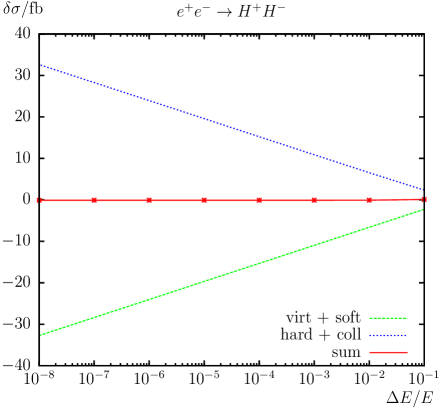
$\Delta E/E$	$\delta\sigma$/fbarn
$10^{-1}$	$0.071\pm 0.001$
$10^{-2}$	$-0.085\pm 0.005$
$10^{-3}$	$-0.099\pm 0.007$
$10^{-4}$	$-0.102\pm 0.009$
$10^{-5}$	$-0.102\pm 0.012$
$10^{-6}$	$-0.098\pm 0.013$
$10^{-7}$	$-0.103\pm 0.019$
$10^{-8}$	$-0.103\pm 0.020$

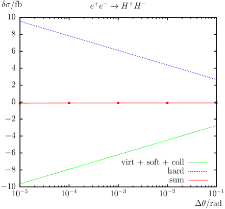
$\Delta\theta$/rad	$\delta\sigma$/fbarn
$10^{0}$	$-0.371\pm 0.008$
$10^{-1}$	$-0.102\pm 0.007$
$10^{-2}$	$-0.099\pm 0.007$
$10^{-3}$	$-0.100\pm 0.007$
$10^{-4}$	$-0.105\pm 0.008$
$10^{-5}$	$-0.116\pm 0.008$
$10^{-6}$	$-0.552\pm 0.010$

Figure 3: Phase space slicing method. the different contributions to the one-loop corrections $\delta\sigma(e^{+}e^{-}\to H^{+}H^{-})$ for our input parameter scenario S1 (see Tab. 2 below) with fixed $\Delta\theta/\text{rad}=10^{-2}$ (upper plot) and fixed $\Delta E/E=10^{-3}$ (lower plot). It should be noted that at $\sqrt{s}=1000\,\,\mathrm{GeV}$ the one-loop corrections are accidentally close to zero in scenario S1 (see Fig. 12 below).

Numerical problems in the phase space integration of the radiative process arise also through collinear photon emission. Mass singularities emerge as a consequence of the collinear photon emission off massless particles. But already very light particles (such as e.g. electrons) can produce numerical instabilities. For the treatment of collinear singularities in the photon radiation off initial state electrons and positrons we used the phase space slicing method [72], which is not (yet) implemented in FormCalc and therefore we have developed and implemented the code necessary for the evaluation of collinear contributions. We have numerically checked that our results do not depend on the angular cut-off parameter $\Delta\theta$ over several orders of magnitude; see the example in the lower plot of Fig. 3. Our numerical results below have been obtained for fixed $\Delta\theta/\text{rad}=10^{-2}$.

The one-loop corrections of the differential cross section are decomposed into the virtual, soft, hard, and collinear parts as follows:

$$\text{d}\sigma_{\text{loop}}=\text{d}\sigma_{\text{virt}}(\lambda)+\text{d}\sigma_{\text{soft}}(\lambda,\Delta E)+\text{d}\sigma_{\text{hard}}(\Delta E,\Delta\theta)+\text{d}\sigma_{\text{coll}}(\Delta E,\Delta\theta)\,.$$ (5)

The hard and collinear parts have been calculated via the Monte Carlo integration algorithm Vegas as implemented in FormCalc.

3 Comparisons

In this section we present the comparisons with results from other groups in the literature for charged Higgs boson production in $e^{+}e^{-}$ collisions. These comparisons were restricted to the MSSM with real parameters, since, to our knowledge, no results for complex parameters have been calculated so far. The level of agreement of such comparisons (at one-loop order) depends on the correct transformation of the input parameters from our renormalization scheme into the schemes used in the respective literature, as well as on the differences in the employed renormalization schemes as such. In view of the non-trivial conversions and the large number of comparisons such transformations and/or change of our renormalization prescription is beyond the scope of our paper.

• In Ref. [43] the process $e^{+}e^{-}\to H^{+}H^{-}$ has been calculated in the rMSSM with third-generation (s)fermion loop corrections. The authors also used FeynArts to generate the corresponding Feynman diagrams. As input parameters we used their parameters as far as possible. For the comparison with Ref. [43] we successfully reproduced their Fig. 1 (tree level). But we disagree with their Fig. 2b (top–bottom contributions), Fig. 3 (top–bottom contributions), Figs. 4a,b (squark, slepton contributions) and their Fig. 5 (“total” one-loop corrections). It should be noted that in Ref. [45] (see also the third item below) the authors revised some of the results of Ref. [43].

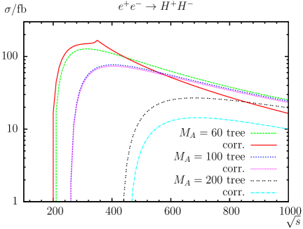
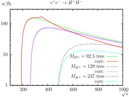
  Figure 4: Comparison with Ref. [44] for $\sigma(e^{+}e^{-}\to H^{+}H^{-})$. Tree and one-loop corrected cross sections are shown with parameters chosen according to Ref. [44] with $\sqrt{s}$ varied. the left (right) plots show cross sections for three different $M_{A}$ ($M_{H^{\pm}}$) masses in GeV.

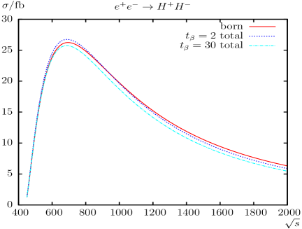
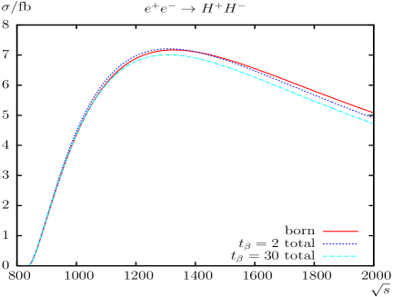
  Figure 5: Comparison with Ref. [45] for $\sigma(e^{+}e^{-}\to H^{+}H^{-})$. Tree and total one-loop cross sections are shown with parameters chosen according to Ref. [45] as a function of $\sqrt{s}$. the left (right) plot shows cross sections for $M_{H^{\pm}}=220$ ($M_{H^{\pm}}=420$) GeV and $t_{\beta}$ varied.

• In Ref. [44] the process $e^{+}e^{-}\to H^{+}H^{-}$ has been calculated in the rMSSM with (s)top/(s)bottom loop corrections. As input parameters we used their parameters as far as possible. For the comparison with Ref. [44] we successfully reproduced their Figs. 2a,b in our Fig. 4 (using also only (s)top/(s)bottom loop corrections). The expected (rather) small differences in the cross sections are likely caused by slightly different SM input parameters and the different renormalization scheme.

• A numerical comparison of $e^{+}e^{-}\to H^{+}H^{-}$ with Ref. [45] can be found in our Fig. 5. They calculated the THDM bosonic and fermionic one-loop contributions of the rMSSM (denoted as $\lambda_{3}^{\text{MSSM}}$ in their plots) including soft photon bremsstrahlung. These contributions have still been missed in their earlier paper [43] (see also the first item). But it should be noted that they finally omitted the soft photon radiation in their “total” one-loop cross sections (as we did for the comparison). Their Feynman diagrams have also been generated with FeynArts. As input we used their parameters in our calculation. In Fig. 5 we show our calculation in comparison to their Figs. 8a,b and 9a,b, where we find very good agreement with their results.

• In Ref. [50] the full one-loop corrections to the process $e^{+}e^{-}\to H^{+}H^{-}$ in the rMSSM have been calculated including hard and soft bremsstrahlung. As input we used their parameter sets A and B. We reproduced their Fig. 1 (tree level), Fig. 2 (QED corrections) and Fig. 4,5 (weak corrections) in our Fig. 6. Explicit numbers have been given in their Tab. 1 which we have reproduced in our Tab. 1. We are in rather good agreement with their results, except for the soft photon radiation. This can be explained with the fact that they have also included higher order contributions into their initial state radiation while we kept our calculation at ${\cal O}(\alpha)$.

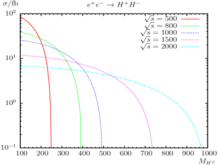
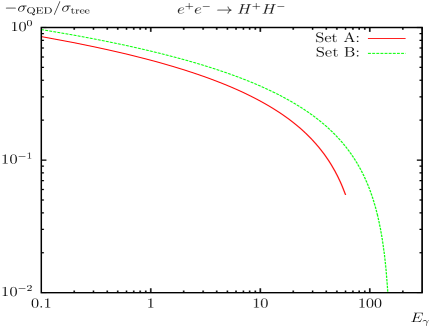
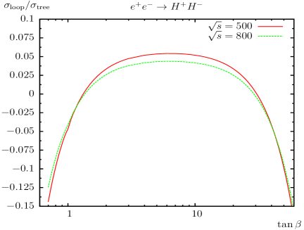
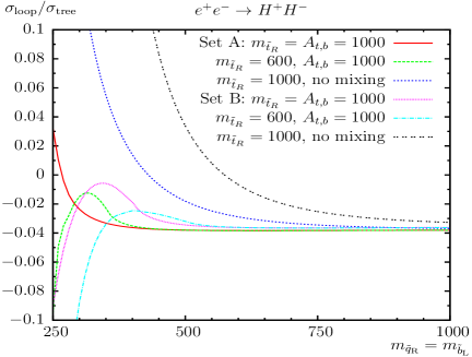
  Figure 6: Comparison with Ref. [50] for $\sigma(e^{+}e^{-}\to H^{+}H^{-})$. Tree and one-loop corrected cross sections are shown with parameters chosen according to Ref. [50]. the upper left (right) plot shows different cross sections (ratios) for $M_{H^{\pm}}$ ($E_{\gamma}$) varied. the lower left (right) plot shows different ratios for $t_{\beta}$ ($m_{\tilde{b}_{L}}$) varied. Masses and energies are in GeV.

  Table 1: Comparison of the one-loop corrected weak Higgs boson production ratios $\sigma_{\text{weak}}/\sigma_{\text{tree}}$ with Ref. [50]. All masses are in GeV.

  					$\sigma_{\text{weak}}/\sigma_{\text{tree}}$
  Set	$t_{\beta}$	$M_{1}$	$m_{{\tilde{l}}_{L}}$	$m_{\mathrm{\tilde{e}}_{R}}$	Ref. [50]	FeynTools
  	40	500	1000	1000	-4.160%	-4.191%
  A	2	1000	100	100	3.414%	3.269%
  	40	500	1000	1000	-4.290%	-4.286%
  B	2	1000	100	100	2.752%	2.716%

• The effect of Sudakov logarithms on $e^{+}e^{-}\to H^{+}H^{-}$ were analyzed in Ref. [52]. Unfortunately, they show mostly plots with $\Delta_{\text{rem}}$, the difference between the full one-loop result and its asymptotic Sudakov expansion (i.e. the next-to subleading term). Nevertheless, using their scenario L, we found rather good agreement with their Fig. 9 where they presented their full effects at $\sqrt{s}=1\,\,\mathrm{TeV}$; see our Fig. 7. The expected (rather small) difference in the ratio is likely caused by slightly different SM input parameters and the different treatment of the loop corrections.

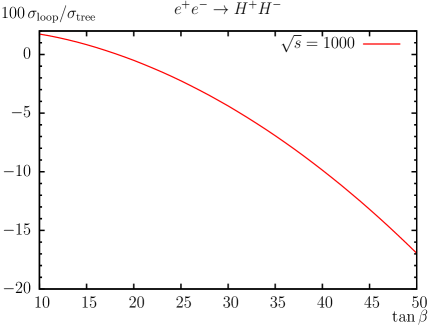
  Figure 7: Comparison with Ref. [52] for $\sigma(e^{+}e^{-}\to H^{+}H^{-})$. the ratio $\sigma_{\text{loop}}/\sigma_{\text{tree}}$ (times a factor of one hundred) is shown with parameters chosen according to Ref. [52] as a function of $t_{\beta}$.

• In Ref. [46] the process $e^{+}e^{-}\to H^{+}H^{-}$ has been calculated in the rMSSM. Unfortunately, in Ref. [46] the numerical evaluation (shown in their Fig. 2) are only tree-level results, although the paper deals with the respective one-loop corrections. For the comparison with Ref. [46] we successfully reproduced their upper Fig. 2.

• In Ref. [53] triple Higgs boson production has been computed with FeynTools. For comparison with their triple Higgs boson results they calculated also $e^{+}e^{-}\to H^{+}H^{-}$ but only at the tree level and for general THDM input parameters. Because our tree level results are already in very good agreement with other groups, we omitted an additional comparison with Ref. [53].

• In Ref. [47] the THDM one-loop contributions of the rMSSM to the process $e^{+}e^{-}\to H^{\pm}W^{\mp}$ have been calculated. We used their input parameters as far as possible and reproduced Fig. 2 and Fig. 3 of Ref. [47] in our Fig. 8, which shows that we are in rather good agreement with Ref. [47].

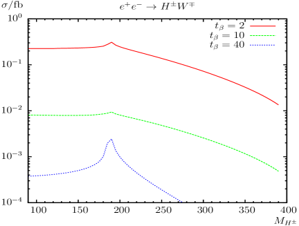
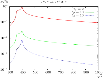
  Figure 8: Comparison with Ref. [47] for $\sigma(e^{+}e^{-}\to H^{\pm}W^{\mp})$. Loop-induced cross sections (in fb) are shown for three different values of $t_{\beta}$ with parameters chosen according to Ref. [47]. the left (right) plot shows cross sections with $M_{H^{\pm}}$ ($\sqrt{s}$) varied.

• The general THDM and the THDM one-loop contributions of the rMSSM to the $H^{\pm}W^{\mp}$ production have been calculated in Ref. [48]. We used their input parameters as far as possible and reproduced their Fig. 3 in our Fig. 9. We are in very good qualitative agreement but we differ quantitatively by a factor 1/2 for the process $e^{+}e^{-}\to H^{-}W^{+}$. Thus we can confirm what the authors of Ref. [51] noted, “that the results in Ref. [48] are the average over the spin states $e^{+}_{L}e^{-}_{R}$ and $e^{+}_{R}e^{-}_{L}$; for unpolarized beams the cross sections should be divided by two”.

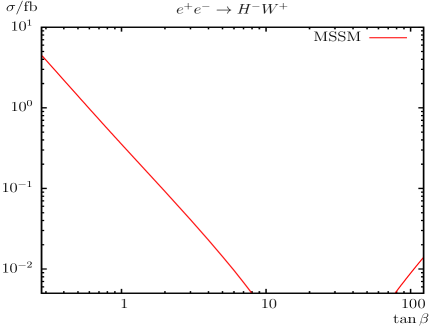
  Figure 9: Comparison with Ref. [48] for $\sigma(e^{+}e^{-}\to H^{-}W^{+})$. Loop-induced cross sections (in fb) are shown with parameters chosen according to Ref. [48] as a function of $t_{\beta}$.

• $e^{+}e^{-}\to H^{\pm}W^{\mp}$ within the general THDM has been analyzed in Ref. [49]. As input parameters they used only the general THDM parameters rendering a comparison rather difficult. In addition a general THDM calculation is beyond the scope of our paper. Consequently, we omitted a comparison with Ref. [49].

• In Ref. [51] the loop induced process $e^{+}e^{-}\to H^{\pm}W^{\mp}$ has been computed in the rMSSM. We used their input parameters as far as possible and are roughly in agreement with their Fig. 7 and Fig. 8; see our Fig. 10, where we show $\sigma(e^{+}e^{-}\to H^{-}W^{+})$. The differences in the cross sections are likely caused by the different SM input parameters and the different renormalization schemes. In addition it should be noted that the authors of Ref. [55] wrote that, “… the results agree, if in Eq. (C14) of Ref. [51] the tensor coefficient $D_{23}$ in the coefficient of ${\cal A}_{6}g^{R}_{W}g^{L}_{H}$ is replaced by $2\,D_{23}$”. Which may also explain some differences in the comparison with Ref. [51].

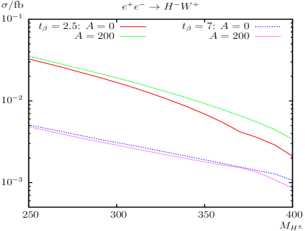
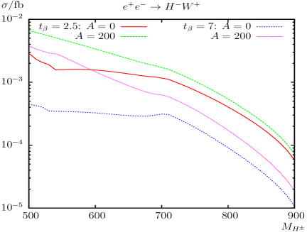
  Figure 10: Comparison with Ref. [51] for $\sigma(e^{+}e^{-}\to H^{-}W^{+})$. Loop-induced cross sections (in fb) are shown with $M_{H^{\pm}}$ varied, with parameters chosen according to Ref. [51]. the left (right) plot shows cross sections for $\sqrt{s}=500\,\,\mathrm{GeV}$ ($\sqrt{s}=1000\,\,\mathrm{GeV}$) with unpolarized beams.

• Ref. [54] is (more or less) an extension to Ref. [51] (see the previous item), dealing with two-dimensional parameter scan plots and ten event contours for $e^{+}e^{-}\to H^{\pm}W^{\mp}$, which we could not reasonably compare to our results. Anyhow, a comparison with Ref. [54] would not give more agreement/understanding as already achieved with Ref. [51]. Consequently, we omitted a comparison with Ref. [54].

• Finally we compared our results for $e^{+}e^{-}\to H^{\pm}W^{\mp}$ with Ref. [55]. They also used (older versions of) FeynTools for their calculations. We are in rather good agreement, in both cases polarized and unpolarized beams; see our Fig. 11 vs. their Figs. 5–7. We also compared successfully (i.e. better than $0.6\%$ agreement) numerical results with code from the co-author [73] of Ref. [55].

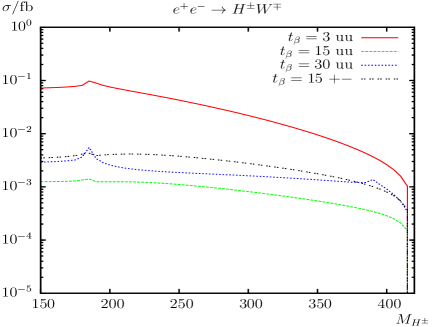
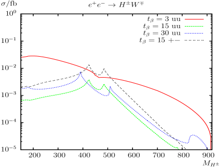
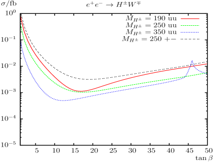
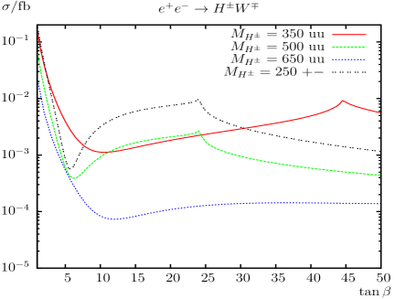
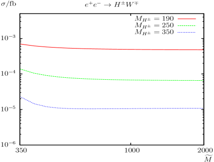
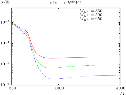
  Figure 11: Comparison with Ref. [55] for $\sigma(e^{+}e^{-}\to H^{\pm}W^{\mp})$. Loop-induced cross sections (in fb) are shown with parameters chosen according to Ref. [55] in the large stop-mixing scenario. the upper, middle, and lower plots show cross sections with $M_{H^{\pm}}$, $t_{\beta}$, and $\widetilde{M}$ varied. the left (right) plots show cross sections at $\sqrt{s}=500\,(1000)\,\,\mathrm{GeV}$.

4 Numerical analysis

In this section we present our numerical analysis of charged Higgs boson production at $e^{+}e^{-}$ colliders in the cMSSM. In the figures below we show the cross sections at the tree level (“tree”) and at the full one-loop level (“full”), which is the cross section including all one-loop corrections as described in Sect. 2. In the case of vanishing tree-level production cross sections we show the purely loop-induced results (“loop”) $\propto|{\cal M}_{\text{1-loop}}|^{2}$, where ${\cal M}_{\text{1-loop}}$ denotes the one-loop matrix element of the appropriate process.

We begin the numerical analysis with the cross sections of $e^{+}e^{-}\to H^{+}H^{-}$ in Sect. 4.2, evaluated as a function of $\sqrt{s}$ (up to $3\,\,\mathrm{TeV}$, shown in the upper left plot of the respective figures), $M_{H^{\pm}}$ (starting at $M_{H^{\pm}}=100\,\,\mathrm{GeV}$ up to $M_{H^{\pm}}=500\,\,\mathrm{GeV}$, shown in the upper right plots), $t_{\beta}$ (from 2 to 50, lower left plots) and $\varphi_{A_{t}}$ (between $0^{\circ}$ and $360^{\circ}$, lower right plots). Then we turn to the processes $e^{+}e^{-}\to H^{\pm}W^{\mp}$ in Sect. 4.3. All these processes are of particular interest for ILC and CLIC analyses [16, 17, 18, 20] (as emphasized in Sect. 1).

4.1 Parameter settings

The renormalization scale $\mu_{R}$ has been set to the center-of-mass energy, $\sqrt{s}$. the SM parameters are chosen as follows; see also [74]:

• Fermion masses (on-shell masses, if not indicated differently):

  $$m_{e} =0.510998928\,\,\mathrm{MeV}\,, m_{\nu_{e}} =0\,,$$

  $$m_{\mu} =105.65837515\,\,\mathrm{MeV}\,, m_{\nu_{\mu}} =0\,,$$

  $$m_{\tau} =1776.82\,\,\mathrm{MeV}\,, m_{\nu_{\tau}} =0\,,$$

  $$m_{u} =73.56\,\,\mathrm{MeV}\,, m_{d} =73.56\,\,\mathrm{MeV}\,,$$

  $$m_{c} =1.275\,\,\mathrm{GeV}\,, m_{s} =95.0\,\,\mathrm{MeV}\,,$$

  $$m_{t} =173.21\,\,\mathrm{GeV}\,, m_{b} =4.66\,\,\mathrm{GeV}\,.$$ (6)

  According to Ref. [74], $m_{s}$ is an estimate of a so-called ”current quark mass” in the $\overline{\mathrm{MS}}$ scheme at the scale $\mu\approx 2\,\,\mathrm{GeV}$. $m_{c}\equiv m_{c}(m_{c})$ is the ”running” mass in the $\overline{\mathrm{MS}}$ scheme and $m_{b}$ is the $\Upsilon(1S)$ bottom quark mass. $m_{u}$ and $m_{d}$ are effective parameters, calculated through the hadronic contributions to

  $$\Delta\alpha_{\text{had}}^{(5)}(M_{Z}) =\frac{\alpha}{\pi}\sum_{f=u,c,d,s,b}Q_{f}^{2}\Bigl{(}\ln\frac{M_{Z}^{2}}{m_{f}^{2}}-\frac{5}{3}\Bigr{)}\approx 0.027547\,.$$ (7)

• Gauge-boson masses:

  $$M_{Z}=91.1876\,\,\mathrm{GeV}\,,\qquad M_{W}=80.385\,\,\mathrm{GeV}\,.$$ (8)

• Coupling constant:

  $$\alpha(0)=1/137.0359895\,.$$ (9)

Table 2: MSSM default parameters for the numerical investigation; all parameters (except of $t_{\beta}$) are in GeV. the values for the trilinear sfermion Higgs couplings, $A_{t,b,\tau}$ are chosen such that charge- and/or color-breaking minima are avoided [75], and $A_{b,\tau}$ are chosen to be real. It should be noted that for the first and second generation of sfermions we chose instead $A_{f}=0$, $M_{\tilde{Q},\tilde{U},\tilde{D}}=1500\,\,\mathrm{GeV}$ and $M_{\tilde{L},\tilde{E}}=500\,\,\mathrm{GeV}$.

Scen.	$\sqrt{s}$	$t_{\beta}$	$\mu$	$M_{H^{\pm}}$	$M_{\tilde{Q},\tilde{U},\tilde{D}}$	$M_{\tilde{L},\tilde{E}}$	$|A_{t,b,\tau}|$	$M_{1}$	$M_{2}$	$M_{3}$
S1	1000	7	200	300	1000	500	$1500+\mu/t_{\beta}$	100	200	1500
S2	800	4	200	300	1000	500	$1500+\mu/t_{\beta}$	100	200	1500

The SUSY parameters are chosen according to the scenarios S1 and S2, shown in Tab. 2. These scenarios are viable for the various cMSSM Higgs boson production modes, i.e. not picking specific parameters for each cross section. They are in particular in agreement with the searches for charged Higgs bosons of ATLAS [76] and CMS [77]. It should be noted that higher-order corrected Higgs boson masses do not enter our calculation. However, we ensured that over larger parts of the parameter space the lightest Higgs boson mass is around $\sim 125\pm 3\,\,\mathrm{GeV}$ to indicate the phenomenological validity of our scenarios. In our numerical evaluation we will show the variation with $\sqrt{s}$, $M_{H^{\pm}}$, $t_{\beta}$, and $\varphi_{A_{t}}$, the phase of $A_{t}$.

Concerning the complex parameters, some more comments are in order. No complex parameter enters into the tree-level production cross sections. Therefore, the largest effects are expected from the complex phases entering via the Higgs sector, i.e. from $\varphi_{A_{t}}$, motivating our choice of $\varphi_{A_{t}}$ as parameter to be varied. Here the following should be kept in mind. When performing an analysis involving complex parameters it should be noted that the results for physical observables are affected only by certain combinations of the complex phases of the parameters $\mu$, the trilinear couplings $A_{f}$ and the gaugino mass parameters $M_{1,2,3}$ [79, 80]. It is possible, for instance, to rotate the phase $\varphi_{M_{2}}$ away. Experimental constraints on the (combinations of) complex phases arise, in particular, from their contributions to electric dipole moments of the electron and the neutron (see Refs. [81, 82] and references therein), of the deuteron [83] and of heavy quarks [84]. While SM contributions enter only at the three-loop level, due to its complex phases the MSSM can contribute already at one-loop order. Large phases in the first two generations of sfermions can only be accommodated if these generations are assumed to be very heavy [85] or large cancellations occur [86]; see, however, the discussion in Ref. [87]. A review can be found in Ref. [88]. Accordingly (using the convention that $\varphi_{M_{2}}=0$, as done in this paper), in particular, the phase $\varphi_{\mu}$ is tightly constrained [89], while the bounds on the phases of the third-generation trilinear couplings are much weaker.

Since now complex parameters can appear in the couplings, contributions from absorptive parts of self-energy type corrections on external legs can arise. the corresponding formulas for an inclusion of these absorptive contributions via finite wave function correction factors can be found in Refs. [57, 60].

The numerical results shown in the next subsections are of course dependent on the choice of the SUSY parameters. Nevertheless, they give an idea of the relevance of the full one-loop corrections.

4.2 The process $e^{+}e^{-}\to H^{+}H^{-}$

The process $e^{+}e^{-}\to H^{+}H^{-}$ is shown in Fig. 12. As a general comment it should be noted that the tree-level production cross section depends solely on SM parameters (and the charged Higgs boson mass); see Eq. (2.2). Consequently, any dependence on SUSY parameters can enter only at the loop-level (except for the charged Higgs boson mass). It should also be noted that for $s\to\infty$ decreasing cross sections $\propto 1/s$ are expected and for $\sqrt{s}\to 2\,M_{H^{\pm}}$ small cross sections are expected (zero for $\sqrt{s}=2\,M_{H^{\pm}}$); see Eq. (2.2). In the analysis of the production cross section as a function of $\sqrt{s}$ (upper left plot) we find the expected behavior: a strong rise close to the production threshold, followed by a decrease with increasing $\sqrt{s}$. We find relative corrections of $\sim-21\%$ around the production threshold where the tree level is very small. Away from the production threshold, loop corrections of $\sim-1\%$ at $\sqrt{s}=1000\,\,\mathrm{GeV}$ are found in both scenarios, S1 and S2 (see Tab. 2). The relative size of loop corrections increase with increasing $\sqrt{s}$ and reach $\sim+9\%$ at $\sqrt{s}=3000\,\,\mathrm{GeV}$. Since only $t_{\beta}$ is (slightly) different in this plot, the results found in S1 and S2 as a function of $\sqrt{s}$ are nearly identical (and indistinguishable in the plot).

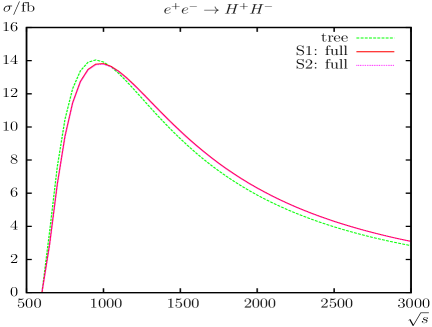
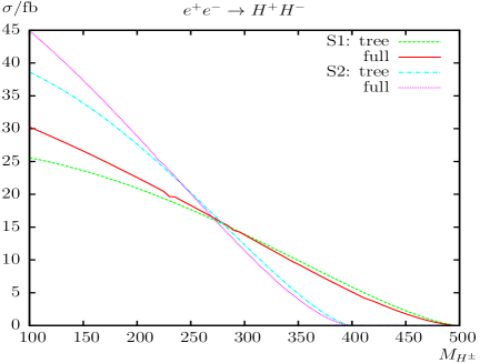
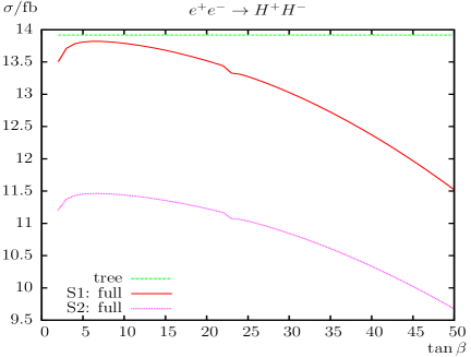
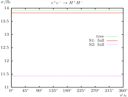
Figure 12: $\sigma(e^{+}e^{-}\to H^{+}H^{-})$. Tree-level and full one-loop corrected cross sections are shown with parameters chosen according to S1 and S2; see Tab. 2. the upper plots show the cross sections with $\sqrt{s}$ (left) and $M_{H^{\pm}}$ (right) varied; the lower plots show $t_{\beta}$ (left) and $\varphi_{A_{t}}$ (right) varied.

With increasing $M_{H^{\pm}}$ in S1 and S2 (upper right plot) we find a strong decrease of the production cross section, as can be expected from kinematics, discussed above. The differences in the tree-level results are purely due to the different choice of $\sqrt{s}$ in our two scenarios. The first dip in S1 (S2) is found at $M_{H^{\pm}}\approx 230\,\,\mathrm{GeV}$ ($M_{H^{\pm}}\approx 221\,\,\mathrm{GeV}$), due to the threshold $m_{\tilde{\chi}_{1}^{\pm}}+m_{\tilde{\chi}_{1}^{0}}=M_{H^{\pm}}$. The second dip can be found at $m_{\tilde{\chi}_{1}^{\pm}}+m_{\tilde{\chi}_{2}^{0}}=M_{H^{\pm}}\approx 290\,\,\mathrm{GeV}$ ($M_{H^{\pm}}\approx 281\,\,\mathrm{GeV}$). The third (hardly visible) dip is at $m_{\tilde{\chi}_{1}^{\pm}}+m_{\tilde{\chi}_{3}^{0}}=M_{H^{\pm}}\approx 350\,\,\mathrm{GeV}$ ($M_{H^{\pm}}\approx 341\,\,\mathrm{GeV}$). The next two dips (hardly visible) are the thresholds at $m_{\tilde{\chi}_{1}^{\pm}}+m_{\tilde{\chi}_{4}^{0}}=M_{H^{\pm}}\approx 412\,\,\mathrm{GeV}$ and $m_{\tilde{\chi}_{2}^{\pm}}+m_{\tilde{\chi}_{2}^{0}}=M_{H^{\pm}}\approx 419\,\,\mathrm{GeV}$. Not visible is the threshold $m_{\tilde{\chi}_{2}^{\pm}}+m_{\tilde{\chi}_{3}^{0}}=M_{H^{\pm}}\approx 478\,\,\mathrm{GeV}$. All these thresholds appear in the vertex and box contributions. The relative loop corrections are very similar in S1 and S2. They reach in S1 (S2) $\sim+18\%$ ($\sim+16\%$) at $M_{H^{\pm}}=100\,\,\mathrm{GeV}$ (experimentally excluded), $\sim-1\%$ ($\sim-7\%$) at $M_{H^{\pm}}=300\,\,\mathrm{GeV}$ and $\sim-45\%$ ($\sim-43\%$) at $M_{H^{\pm}}=490\,\,\mathrm{GeV}$ ($M_{H^{\pm}}=390\,\,\mathrm{GeV}$). These large loop corrections are again due to the (relative) smallness of the tree-level results, which goes to zero for $M_{H^{\pm}}=500\,\,\mathrm{GeV}$ ($M_{H^{\pm}}=400\,\,\mathrm{GeV}$).

The cross section as a function of $t_{\beta}$ is shown in the lower left plot of Fig. 12. the tree-level result is again identical in S1 and S2. First a small increase up to $t_{\beta}\sim 6$ can be observed. For larger values of $t_{\beta}$ the production cross sections goes down by $\sim 20\%$. the loop corrections reach the maximum of $\sim-17\%$ ($\sim-22\%$) at $t_{\beta}=50$ while the minimum of $\sim-1\%$ ($\sim-7\%$) is around $t_{\beta}=6$ in scenario S1 (S2). the dip at $t_{\beta}\approx 23$ is due to the threshold $m_{\tilde{\chi}_{1}^{\pm}}+m_{\tilde{\chi}_{2}^{0}}=M_{H^{\pm}}$.

Due to the absence of SUSY parameters in the tree-level production cross section the effect of complex phases of the SUSY parameters is expected to be small. Correspondingly we find that the phase dependence $\varphi_{A_{t}}$ of the cross section in both scenarios is indeed tiny (lower right plot). The loop corrections are found to be nearly independent of $\varphi_{A_{t}}$ at the level below $\sim-1\%$ ($\sim-7\%$) in S1 (S2).

Overall, for the charged Higgs boson pair production we observed an decreasing cross section $\propto 1/s$ for $s\to\infty$; see Eq. (2.2). The full one-loop corrections are very roughly of ${\cal O}(10\%)$, but can go up to be larger than $\sim 40\%$, where cross sections of $0.1$–$14$ fb have been found. the variation with $\varphi_{A_{t}}$ is found extremely small and the dependence on other phases were found to be roughly at the same level and have not been shown explicitely. The results for $H^{+}H^{-}$ production turn out to be small, for Higgs boson masses above $\sim 350\,\,\mathrm{GeV}$.

4.3 The process $e^{+}e^{-}\to H^{\pm}W^{\mp}$

In Fig. 13 we show the results for the processes $e^{+}e^{-}\to H^{\pm}W^{\mp}$ as before as a function of $\sqrt{s}$, $M_{H^{\pm}}$, $t_{\beta}$ and $\varphi_{A_{t}}$. As discussed above, $e^{+}e^{-}\to H^{\pm}W^{\mp}$ is a purely loop-induced process (via vertex and box diagrams) and therefore $\propto|{\cal M}_{\text{1-loop}}|^{2}$. The largest contributions are expected from loops involving top quarks and SM gauge bosons. If not indicated otherwise, unpolarized electrons and positrons are assumed. We also remind the reader that $\sigma(e^{+}e^{-}\to H^{\pm}W^{\mp})$ denotes the sum of the two charge conjugated processes; see Eq. (4).

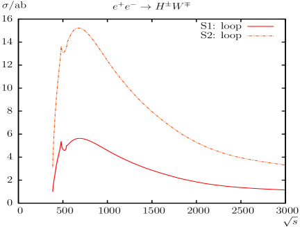
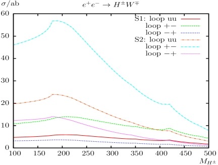
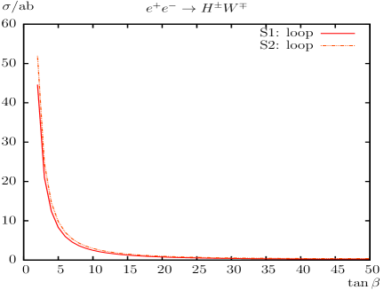
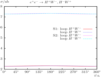
Figure 13: $\sigma(e^{+}e^{-}\to H^{\pm}W^{\mp})$. Loop-induced (i.e. leading two-loop corrected) cross sections are shown with parameters chosen according to S1 and S2 (see Tab. 2). the upper plots show the cross sections with $\sqrt{s}$ (left) and $M_{H^{\pm}}$ (right) varied; the lower plots show $t_{\beta}$ (left) and $\varphi_{A_{t}}$ (right) varied. u denotes unpolarized, $+$ right-, and $-$ left-circular polarized electrons and/or positrons (see text).

The cross section, as shown in Fig. 13, is rather small for the parameter set chosen; see Tab. 2. As a function of $\sqrt{s}$ (upper left plot) a maximum of $\sim 5.6~{}(15)$ ab is reached around $\sqrt{s}\sim 600\,\,\mathrm{GeV}$ in S1 (S2). Two threshold effects partially overlap around $\sqrt{s}\sim 500\,\,\mathrm{GeV}$ independent of the scenario. The first (large) peak is found at $\sqrt{s}\approx 479\,\,\mathrm{GeV}$, due to the threshold $m_{\tilde{\chi}_{3}^{0}}+m_{\tilde{\chi}_{4}^{0}}=\sqrt{s}$. the second (very small) peak can be found at $m_{\tilde{\chi}_{2}^{\pm}}+m_{\tilde{\chi}_{2}^{\pm}}=\sqrt{s}\approx 540\,\,\mathrm{GeV}$. The loop-induced production cross section decreases as a function of $\sqrt{s}$, down to 1.2 (2.4) ab at $\sqrt{s}=3\,\,\mathrm{TeV}$ in S1 (S2). Consequently, this process will hardly be observable also for larger ranges of $\sqrt{s}$. In particular even in the initial phase with $\sqrt{s}=500\,\,\mathrm{GeV}$ only $\sim$ 6 (15) events could be produced.

As a function of $M_{H^{\pm}}$ (upper right plot) we find a maximum production cross section at $M_{H^{\pm}}\approx 200\,\,\mathrm{GeV}$ of $\sim$ 6 (24) ab in S1 (S2). With polarized positrons ($P(e^{+})=+30\%$) and electrons ($P(e^{-})=-80\%$) cross sections up to $\sim$ 56 ab are possible in S2. With this initial state a cross section larger than $\sim 10$ ab is found for nearly the entire displayed range for $M_{H^{\pm}}$, i.e. with $1\,\mbox{ab}^{-1}$ up to 10 events could be collected, which could lead to experimental observation of this process. We also show the results for $P(e^{+})=-30\%$, $P(e^{-})=+80\%$, which results in a decrease of the production cross section. These results indicate that using polarized beams could turn out to be crucial for the observation of this channel.

The production cross section decreases with growing $M_{H^{\pm}}$, yielding values below 2 (4) ab in the decoupling regime [91]. The following thresholds appear in both scenarios. The first peak (not visible in S1, large in S2) is found at $M_{H^{\pm}}\approx 178\,\,\mathrm{GeV}$, due to the threshold $m_{t}+m_{b}=M_{H^{\pm}}$. The second (very small) peak is found at $M_{H^{\pm}}\approx 230\,\,\mathrm{GeV}$, due to the threshold $m_{\tilde{\chi}_{1}^{\pm}}+m_{\tilde{\chi}_{1}^{0}}=M_{H^{\pm}}$. the third (small) peak can be found at $m_{\tilde{\chi}_{1}^{\pm}}+m_{\tilde{\chi}_{3}^{0}}=M_{H^{\pm}}\approx 350\,\,\mathrm{GeV}$. the next (large) peak is in reality the two thresholds at $m_{\tilde{\chi}_{1}^{\pm}}+m_{\tilde{\chi}_{4}^{0}}=M_{H^{\pm}}\approx 412\,\,\mathrm{GeV}$ and $m_{\tilde{\chi}_{2}^{\pm}}+m_{\tilde{\chi}_{2}^{0}}=M_{H^{\pm}}\approx 419\,\,\mathrm{GeV}$. the last (hardly visible) peak at $M_{H^{\pm}}\approx 478\,\,\mathrm{GeV}$ is the threshold $m_{\tilde{\chi}_{2}^{\pm}}+m_{\tilde{\chi}_{3}^{0}}=M_{H^{\pm}}$. All these thresholds appear in the vertex and box contributions and here in addition in the $W^{\pm}$–$H^{\pm}$ self-energy contribution on the external charged Higgs boson.

The cross sections decrease rapidly with increasing $t_{\beta}$ for both scenarios (lower left plot), and the loop corrections reach the maximum of $\sim$ 50 ab at $t_{\beta}=2$ while the minimum of $\sim$ 0.2 ab is at $t_{\beta}=50$.

Finally, the variation with $\varphi_{A_{t}}$ is analyzed. For complex parameters a difference in $\sigma(e^{+}e^{-}\to H^{+}W^{-})$ and $\sigma(e^{+}e^{-}\to H^{-}W^{+})$ is expected. The results for the two channels are shown in the lower right plot of Fig. 13. We find, in agreement with the previous plots, very small values around $\sim$ 2 (7) ab in S1 (S2). The variation with $\varphi_{A_{t}}$ turns out to be tiny (but is non-zero). Similarly, the differences between the $H^{+}W^{-}$ and $H^{-}W^{+}$ final states is found to be extremely small (but non-zero).

Overall, for the $W$–Higgs boson production the leading order corrections can reach a level of ${\cal O}(10)$ ab, depending on the SUSY parameters. This renders these loop-induced processes difficult to observe at an $e^{+}e^{-}$ collider. Having both beams polarized could turn out to be crucial to yield a detectable production cross section. The variation with $\varphi_{A_{t}}$ is found to be extremely small and the dependence on other phases were found to be roughly at the same level and have not been shown explicitely.

5 Conclusions

We evaluated all charged MSSM Higgs boson production modes at $e^{+}e^{-}$ colliders with a two-particle final state, i.e. $e^{+}e^{-}\to H^{+}H^{-}$ and $e^{+}e^{-}\to H^{\pm}W^{\mp}$ allowing for complex parameters. In the case of a discovery of additional Higgs bosons a subsequent precision measurement of their properties will be crucial to determine their nature and the underlying (SUSY) parameters. In order to yield a sufficient accuracy, one-loop corrections to the various charged Higgs boson production modes have to be considered. This is particularly the case for the high anticipated accuracy of the Higgs boson property determination at $e^{+}e^{-}$ colliders [19].

The evaluation of the processes (1) and (2) is based on a full one-loop calculation, also including hard and soft QED radiation. the renormalization is chosen to be identical as for the various Higgs boson decay calculations; see, e.g., Refs. [23, 24, 42].

We first very briefly reviewed the relevant sectors including some details of the one-loop renormalization procedure of the cMSSM, which are relevant for our calculation. In most cases we follow Ref. [57]. We have discussed the calculation of the one-loop diagrams, the treatment of UV, IR, and collinear divergences that are canceled by the inclusion of (hard, soft, and collinear) QED radiation. We have checked our result against the literature as far as possible, and in most cases we found good (or at least acceptable) agreement, where parts of the differences can be attributed to problems with input parameters and/or different renormalization schemes (conversions). Once our set-up was changed successfully to the one used in the existing analyses we found good agreement.

For the analysis we have chosen a standard parameter set (see Tab. 2) that had been used for the analysis of neutral Higgs boson production [42] before. In the analysis we investigated the variation of the various production cross sections with the center-of-mass energy $\sqrt{s}$, the charged Higgs boson mass $M_{H^{\pm}}$, the ratio of the vacuum expectation values $t_{\beta}$ and the phase of the trilinear Higgs–top squark coupling $\varphi_{A_{t}}$. The default values for the center-of-mass energy have been $\sqrt{s}=800,1000\,\,\mathrm{GeV}$.

In our numerical scenarios in the case of $e^{+}e^{-}\to H^{+}H^{-}$ we compared the tree-level production cross sections with the full one-loop corrected cross sections. We found sizable corrections of $\sim 10\%$, but substantially larger corrections are found in cases where the tree-level result is small, e.g. due to kinematical restrictions. The purely loop-induced processes of $e^{+}e^{-}\to H^{\pm}W^{\mp}$ are very challenging to be detected. Polarized initial state electrons/positrons could turn out to be crucial to increase the cross section to an observable level.

Concerning the complex phases of the cMSSM, no relevant dependence on $\varphi_{A_{t}}$ was found. the dependence on other phases were found to be roughly at the same level and have not been shown explicitely.

The numerical results we have shown are, of course, dependent on the choice of the SUSY parameters. Nevertheless, they give an idea of the relevance of the full one-loop corrections. Following our analysis it is evident that the full one-loop corrections for $e^{+}e^{-}\to H^{+}H^{-}$ are mandatory for a precise prediction of the various cMSSM Higgs boson production processes, and that the loop-induced process $e^{+}e^{-}\to H^{\pm}W^{\mp}$ should not be discarded from the start. Consequently, the full one-loop cross section evaluations must be taken into account in any precise determination of (SUSY) parameters from the production of cMSSM Higgs bosons at $e^{+}e^{-}$ linear colliders.

Acknowledgements

We thank T. Hahn, W. Hollik, S. Liebler and F. von der Pahlen for helpful discussions. The work of S.H. is supported in part by CICYT (Grant FPA 2013-40715-P) and by the Spanish MICINN’s Consolider-Ingenio 2010 Program under Grant MultiDark CSD2009-00064.

References

- [1] G. Aad et al. [ATLAS Collaboration], Phys. Lett. B 716 (2012) 1 [arXiv:1207.7214 [hep-ex]].
- [2] S. Chatrchyan et al. [CMS Collaboration], Phys. Lett. B 716 (2012) 30 [arXiv:1207.7235 [hep-ex]].
-
[3]
S. Zens, talk given at “Rencontres de Moriond EW 2016”, see:
https://indico.in2p3.fr/event/12279/session/5/contribution/176/material/slides/0.pdf ;
L. Dell’Asta, talk given at “Rencontres de Moriond EW 2016”, see: https://indico.in2p3.fr/event/12279/session/5/contribution/202/material/slides/0.pdf . -
[4]
H. Nilles,
Phys. Rept. 110 (1984) 1;
R. Barbieri, Riv. Nuovo Cim. 11 (1988) 1. - [5] H. Haber, G. Kane, Phys. Rept. 117 (1985) 75.
- [6] J. Gunion, H. Haber, Nucl. Phys. B 272 (1986) 1.
-
[7]
A. Pilaftsis,
Phys. Rev. D 58 (1998) 096010
[arXiv:hep-ph/9803297];
A. Pilaftsis, Phys. Lett. B 435 (1998) 88 [arXiv:hep-ph/9805373]. - [8] D. Demir, Phys. Rev. D 60 (1999) 055006 [arXiv:hep-ph/9901389].
- [9] A. Pilaftsis and C. Wagner, Nucl. Phys. B 553 (1999) 3 [arXiv:hep-ph/9902371].
- [10] S. Heinemeyer, Eur. Phys. J. C 22 (2001) 521 [arXiv:hep-ph/0108059].
- [11] S. Heinemeyer, O. Stål and G. Weiglein, Phys. Lett. B 710 (2012) 201 [arXiv:1112.3026 [hep-ph]].
- [12] G. Aad et al. [ATLAS and CMS Collaborations], Phys. Rev. Lett. 114 (2015) 191803 [arXiv:1503.07589 [hep-ex]].
- [13] G. Aad et al. [ATLAS Collaboration], JHEP 1411 (2014) 056 [arXiv:1409.6064 [hep-ex]].
- [14] V. Khachatryan et al. [CMS Collaboration], JHEP 1410 (2014) 160 [arXiv:1408.3316 [hep-ex]].
- [15] A. Holzner [ATLAS and CMS Collaborations], arXiv:1411.0322 [hep-ex].
- [16] H. Baer et al., The International Linear Collider Technical Design Report - Volume 2: Physics, arXiv:1306.6352 [hep-ph].
-
[17]
TESLA Technical Design Report [TESLA Collaboration] Part 3,
Physics at an Linear Collider,
arXiv:hep-ph/0106315,
see: http://tesla.desy.de/new_pages/TDR_CD/start.html ;
K. Ackermann et al., DESY-PROC-2004-01. -
[18]
J. Brau et al. [ILC Collaboration],
ILC Reference Design Report Volume 1 - Executive Summary,
arXiv:0712.1950 [physics.acc-ph];
G. Aarons et al. [ILC Collaboration], International Linear Collider Reference Design Report Volume 2: Physics at the ILC, arXiv:0709.1893 [hep-ph]. - [19] G. Moortgat-Pick et al., Eur. Phys. J. C 75 (2015) 8, 371 [arXiv:1504.01726 [hep-ph]].
-
[20]
L. Linssen, A. Miyamoto, M. Stanitzki and H. Weerts,
arXiv:1202.5940 [physics.ins-det];
H. Abramowicz et al. [CLIC Detector and Physics Study Collaboration], Physics at the CLIC Linear Collider – Input to the Snowmass process 2013, arXiv:1307.5288 [hep-ex]. -
[21]
G. Weiglein et al. [LHC/ILC Study Group],
Phys. Rept. 426 (2006) 47
[arXiv:hep-ph/0410364];
A. De Roeck et al., Eur. Phys. J. C 66 (2010) 525 [arXiv:0909.3240 [hep-ph]];
A. De Roeck, J. Ellis and S. Heinemeyer, CERN Cour. 49N10 (2009) 27. - [22] K. Williams, H. Rzehak, and G. Weiglein, Eur. Phys. J. C 71 (2011) 1669 [arXiv:1103.1335 [hep-ph]].
- [23] S. Heinemeyer and C. Schappacher, Eur. Phys. J. C 75 (2015) 5, 198 [arXiv:1410.2787 [hep-ph]].
- [24] S. Heinemeyer and C. Schappacher, Eur. Phys. J. C 75 (2015) 5, 230 [arXiv:1503.02996 [hep-ph]].
- [25] S. Heinemeyer, W. Hollik and G. Weiglein, Eur. Phys. J. C 16 (2000) 139 [arXiv:hep-ph/0003022].
-
[26]
R. Hempfling,
Phys. Rev. D 49 (1994) 6168;
L. Hall, R. Rattazzi and U. Sarid, Phys. Rev. D 50 (1994) 7048 [arXiv:hep-ph/9306309];
M. Carena, M. Olechowski, S. Pokorski and C. Wagner, Nucl. Phys. B 426 (1994) 269 [arXiv:hep-ph/9402253];
M. Carena, D. Garcia, U. Nierste and C. Wagner, Nucl. Phys. B 577 (2000) 577 [arXiv:hep-ph/9912516]. - [27] D. Noth and M. Spira, Phys. Rev. Lett. 101 (2008) 181801 [arXiv:0808.0087 [hep-ph]]; JHEP 1106 (2011) 084 [arXiv:1001.1935 [hep-ph]].
- [28] V. Barger, M. Berger, A. Stange and R. Phillips, Phys. Rev. D 45 (1992) 4128.
- [29] S. Heinemeyer and W. Hollik, Nucl. Phys. B 474 (1996) 32 [arXiv:hep-ph/9602318].
- [30] W. Hollik and J. Zhang, Phys. Rev. D 84 (2011) 055022 [arXiv:1109.4781 [hep-ph]].
-
[31]
A. Bredenstein, A. Denner, S. Dittmaier and M. Weber,
Phys. Rev. D 74 (2006) 013004
[arXiv:hep-ph/0604011];
JHEP 0702 (2007) 080
[arXiv:hep-ph/0611234];
A. Bredenstein, A. Denner, S. Dittmaier, A. Mück and M. Weber,
see: http://omnibus.uni-freiburg.de/~sd565/programs/prophecy4f/prophecy4f.html . - [32] M. Frank, T. Hahn, S. Heinemeyer, W. Hollik, H. Rzehak and G. Weiglein, JHEP 0702 (2007) 047 [arXiv:hep-ph/0611326].
-
[33]
S. Heinemeyer, W. Hollik and G. Weiglein,
Comput. Phys. Commun. 124 (2000) 76
[arXiv:hep-ph/9812320];
T. Hahn, S. Heinemeyer, W. Hollik, H. Rzehak and G. Weiglein, Comput. Phys. Commun. 180 (2009) 1426, see: http://www.feynhiggs.de . - [34] S. Heinemeyer, W. Hollik and G. Weiglein, Eur. Phys. J. C 9 (1999) 343 [arXiv:hep-ph/9812472].
- [35] G. Degrassi, S. Heinemeyer, W. Hollik, P. Slavich and G. Weiglein, Eur. Phys. J. C 28 (2003) 133 [arXiv:hep-ph/0212020].
- [36] T. Hahn, S. Heinemeyer, W. Hollik, H. Rzehak and G. Weiglein, Phys. Rev. Lett. 112 (2014) 141801 [arXiv:1312.4937 [hep-ph]].
-
[37]
A. Djouadi, J. Kalinowsli and M. Spira,
Comput. Phys. Commun. 108 (1998) 56
[arXiv:hep-ph/9704448];
M. Spira, Fortschr. Phys. 46 (1998) 203 [arXiv:hep-ph/9705337]. - [38] A. Djouadi, J. Kalinowski, M. Mühlleitner and M. Spira, arXiv:1003.1643 [hep-ph].
- [39] S. Heinemeyer et al. [LHC Higgs Cross Section Working Group], arXiv:1307.1347 [hep-ph].
-
[40]
R. Harlander, S. Liebler and H. Mantler,
Comput. Phys. Commun. 184 (2013) 1605
[arXiv:1212.3249 [hep-ph]];
E. Bagnaschi, R. Harlander, S. Liebler, H. Mantler, P. Slavich and A. Vicini, JHEP 1406 (2014) 167 [arXiv:1404.0327 [hep-ph]]. - [41] R. Harlander, S. Liebler and H. Mantler, arXiv:1605.03190 [hep-ph].
- [42] S. Heinemeyer and C. Schappacher, Eur. Phys. J. C 76 (2016) 4, 220 [arXiv:1511.06002 [hep-ph]].
- [43] A. Arhrib, M. Capdequi Peyranère and G. Moultaka, Phys. Lett. B 341 (1995) 313 [arXiv:hep-ph/9406357].
- [44] M. Dìaz and T. ter Veldhuis, arXiv:hep-ph/9501315.
- [45] A. Arhrib and G. Moultaka, Nucl. Phys. B 558 (1999) 3 [arXiv:hep-ph/9808317].
- [46] M. Beccaria, A. Ferrari, F. Renard and C. Verzegnassi, arXiv:hep-ph/0506274.
- [47] S. Zhu, arXiv:hep-ph/9901221.
- [48] S. Kanemura, Eur. Phys. J. C 17 (2000) 473 [arXiv:hep-ph/9911541].
- [49] A. Arhrib, M. Capdequi Peyranère, W. Hollik and G. Moultaka, Nucl. Phys. B 581 (2000) 34, [Erratum-ibid. B 679 (2004) 400] [arXiv:hep-ph/9912527].
- [50] J. Guasch, W. Hollik and A. Kraft, Nucl. Phys. B 596 (2001) 66 [arXiv:hep-ph/9911452].
- [51] H. Logan and S. Su, Phys. Rev. D 66 (2002) 035001 [arXiv:hep-ph/0203270].
- [52] M. Beccaria, F. Renard, S. Trimarchi and C. Verzegnassi, Phys. Rev. D 68 (2003) 035014 [arXiv:hep-ph/0212167].
- [53] G. Ferrera, J. Guasch, D. Lopez-Val and J. Sola, Phys. Lett. B 659 (2008) 297 [arXiv:0707.3162 [hep-ph]].
- [54] H. Logan and S. Su, Phys. Rev. D 67 (2003) 017703 [arXiv:hep-ph/0206135].
- [55] O. Brein and T. Hahn, Eur. Phys. J. C 52 (2007) 397 [arXiv:hep-ph/0610079].
-
[56]
J. Küblbeck, M. Böhm and A. Denner,
Comput. Phys. Commun. 60 (1990) 165;
T. Hahn, Comput. Phys. Commun. 140 (2001) 418 [arXiv:hep-ph/0012260];
T. Hahn and C. Schappacher, Comput. Phys. Commun. 143 (2002) 54 [arXiv:hep-ph/0105349].
Program, user’s guide and model files are available via: http://www.feynarts.de . - [57] T. Fritzsche, T. Hahn, S. Heinemeyer, F. von der Pahlen, H. Rzehak and C. Schappacher, Comput. Phys. Commun. 185 (2014) 1529 [arXiv:1309.1692 [hep-ph]].
- [58] T. Hahn and M. Pérez-Victoria, Comput. Phys. Commun. 118 (1999) 153 [arXiv:hep-ph/9807565].
- [59] S. Heinemeyer, H. Rzehak and C. Schappacher, Phys. Rev. D 82 (2010) 075010 [arXiv:1007.0689 [hep-ph]]; PoSCHARGED 2010 (2010) 039 [arXiv:1012.4572 [hep-ph]].
- [60] T. Fritzsche, S. Heinemeyer, H. Rzehak and C. Schappacher, Phys. Rev. D 86 (2012) 035014 [arXiv:1111.7289 [hep-ph]].
- [61] S. Heinemeyer and C. Schappacher, Eur. Phys. J. C 72 (2012) 1905 [arXiv:1112.2830 [hep-ph]].
- [62] S. Heinemeyer and C. Schappacher, Eur. Phys. J. C 72 (2012) 2136 [arXiv:1204.4001 [hep-ph]].
- [63] S. Heinemeyer, F. von der Pahlen and C. Schappacher, Eur. Phys. J. C 72 (2012) 1892 [arXiv:1112.0760 [hep-ph]]; arXiv:1202.0488 [hep-ph].
- [64] A. Bharucha, S. Heinemeyer, F. von der Pahlen and C. Schappacher, Phys. Rev. D 86 (2012) 075023 [arXiv:1208.4106 [hep-ph]].
- [65] A. Bharucha, S. Heinemeyer and F. von der Pahlen, Eur. Phys. J. C 73 (2013) 2629 [arXiv:1307.4237 [hep-ph]].
- [66] A. Denner, S. Dittmaier, M. Roth and D. Wackeroth, Nucl. Phys. B 560 (1999) 33 [hep-ph/9904472].
- [67] F. del Aguila, A. Culatti, R. Muñoz Tapia and M. Pérez-Victoria, Nucl. Phys. B 537 (1999) 561 [arXiv:hep-ph/9806451].
-
[68]
W. Siegel,
Phys. Lett. B 84 (1979) 193;
D. Capper, D. Jones, and P. van Nieuwenhuizen, Nucl. Phys. B 167 (1980) 479. - [69] D. Stöckinger, JHEP 0503 (2005) 076 [arXiv:hep-ph/0503129].
- [70] W. Hollik and D. Stöckinger, Phys. Lett. B 634 (2006) 63 [arXiv:hep-ph/0509298].
- [71] A. Denner, Fortsch. Phys. 41 (1993) 307 [arXiv:0709.1075 [hep-ph]].
-
[72]
K. Fabricius, I. Schmitt, G. Kramer and G. Schierholz,
Zeit. Phys. C 11 (1981) 315;
G. Kramer and B. Lampe, Fortschr. Phys. 37 (1989) 161;
H. Baer, J. Ohnemus and J. Owens, Phys. Rev. D 40 (1989) 2844;
B. Harris and J. Owens, Phys. Rev. D 65 (2002) 094032 [arXiv:hep-ph/0102128]. - [73] T. Hahn, private communication, 03.06.2016.
- [74] K. Olive et al. (Particle Data Group), Chin. Phys. C 38 (2014) 090001.
-
[75]
J. Frère, D. Jones and S. Raby,
Nucl. Phys. B 222 (1983) 11;
M. Claudson, L. Hall and I. Hinchliffe, Nucl. Phys. B 228 (1983) 501;
C. Kounnas, A. Lahanas, D. Nanopoulos and M. Quiros, Nucl. Phys. B 236 (1984) 438;
J. Gunion, H. Haber and M. Sher, Nucl. Phys. B 306 (1988) 1;
J. Casas, A. Lleyda and C. Muñoz, Nucl. Phys. B 471 (1996) 3 [arXiv:hep-ph/9507294];
P. Langacker and N. Polonsky, Phys. Rev. D 50 (1994) 2199 [arXiv:hep-ph/9403306];
A. Strumia, Nucl. Phys. B 482 (1996) 24 [arXiv:hep-ph/9604417]. -
[76]
G. Aad et al. [ATLAS Collaboration],
JHEP 1503 (2015) 088
[arXiv:1412.6663 [hep-ex]];
JHEP 1603 (2016) 127
[arXiv:1512.03704 [hep-ex]];
M. Aaboud et al. [ATLAS Collaboration], arXiv:1603.09203 [hep-ex]. -
[77]
CMS Collaboration [CMS Collaboration],
CMS-PAS-HIG-13-026;
V. Khachatryan et al. [CMS Collaboration], JHEP 1511 (2015) 018 [arXiv:1508.07774 [hep-ex]]; JHEP 1512 (2015) 178 [arXiv:1510.04252 [hep-ex]]. - [78] M. Frank et al., Phys. Rev. D 88 (2013) 5, 055013 [arXiv:1306.1156 [hep-ph]].
- [79] S. Dimopoulos and S. Thomas, Nucl. Phys. B 465 (1996) 23 [arXiv:hep-ph/9510220].
- [80] M. Dugan, B. Grinstein and L. Hall, Nucl. Phys. B 255 (1985) 413.
- [81] D. Demir, O. Lebedev, K. Olive, M. Pospelov and A. Ritz, Nucl. Phys. B 680 (2004) 339 [arXiv:hep-ph/0311314].
-
[82]
D. Chang, W. Keung and A. Pilaftsis,
Phys. Rev. Lett. 82 (1999) 900
[Erratum-ibid. 83 (1999) 3972]
[arXiv:hep-ph/9811202];
A. Pilaftsis, Phys. Lett. B 471 (1999) 174 [arXiv:hep-ph/9909485]. - [83] O. Lebedev, K. Olive, M. Pospelov and A. Ritz, Phys. Rev. D 70 (2004) 016003 [arXiv:hep-ph/0402023].
- [84] W. Hollik, J. Illana, S. Rigolin and D. Stöckinger, Phys. Lett. B 416 (1998) 345 [arXiv:hep-ph/9707437]; Phys. Lett. B 425 (1998) 322 [arXiv:hep-ph/9711322].
-
[85]
P. Nath,
Phys. Rev. Lett. 66 (1991) 2565;
Y. Kizukuri and N. Oshimo, Phys. Rev. D 46 (1992) 3025. -
[86]
T. Ibrahim and P. Nath,
Phys. Lett. B 418 (1998) 98
[arXiv:hep-ph/9707409];
Phys. Rev. D 57 (1998) 478
[Erratum-ibid. D 58 (1998) 019901]
[Erratum-ibid. D 60 (1998) 079903]
[Erratum-ibid. D 60 (1999) 119901]
[arXiv:hep-ph/9708456];
M. Brhlik, G. Good and G. Kane, Phys. Rev. D 59 (1999) 115004 [arXiv:hep-ph/9810457]. - [87] S. Abel, S. Khalil and O. Lebedev, Nucl. Phys. B 606 (2001) 151 [arXiv:hep-ph/0103320].
- [88] Y. Li, S. Profumo and M. Ramsey-Musolf, JHEP 1008 (2010) 062 [arXiv:1006.1440 [hep-ph]].
- [89] V. Barger, T. Falk, T. Han, J. Jiang, T. Li and T. Plehn, Phys. Rev. D 64 (2001) 056007 [arXiv:hep-ph/0101106].
- [90] T. Barklow, et al. arXiv:1506.07830 [hep-ex].
-
[91]
A. Dobado, M. Herrero and S. Peñaranda,
Eur. Phys. J. C 17 (2000) 487
[arXiv:hep-ph/0002134];
J. Gunion and H. Haber, Phys. Rev. D 67 (1993) 075019 [arXiv:hep-ph/0207010];
H. Haber and Y. Nir, Phys. Lett. B 306 (1993) 327 [arXiv:hep-ph/9302228];
H. Haber, arXiv:hep-ph/9505240.