Computing hypergeometric functions rigorously

Abstract

We present an efficient implementation of hypergeometric functions in arbitrary-precision interval arithmetic. The functions ${}_{0}F_{1}$, ${}_{1}F_{1}$, ${}_{2}F_{1}$ and ${}_{2}F_{0}$ (or the Kummer $U$-function) are supported for unrestricted complex parameters and argument, and by extension, we cover exponential and trigonometric integrals, error functions, Fresnel integrals, incomplete gamma and beta functions, Bessel functions, Airy functions, Legendre functions, Jacobi polynomials, complete elliptic integrals, and other special functions. The output can be used directly for interval computations or to generate provably correct floating-point approximations in any format. Performance is competitive with earlier arbitrary-precision software, and sometimes orders of magnitude faster. We also partially cover the generalized hypergeometric function ${}_{p}F_{q}$ and computation of high-order parameter derivatives.

1 Introduction

Naive numerical methods for evaluating special functions are prone to give inaccurate results, particularly in the complex domain. Ensuring just a few correct digits in double precision (53-bit) floating-point arithmetic can be hard, and many scientific applications require even higher accuracy [3]. To give just a few examples, Bessel functions are needed with quad precision (113-bit) accuracy in some electromagnetics and hydrogeophysics simulations [61, 40], with hundreds of digits in integer relation searches such as for Ising class integrals [4], and with thousands of digits in number theory for computing with L-functions and modular forms [8].

In this work, we address evaluation of the confluent hypergeometric functions ${}_{0}F_{1}$, ${}_{1}F_{1}$ and ${}_{2}F_{0}$ (equivalently, the Kummer $U$-function) and the Gauss hypergeometric function ${}_{2}F_{1}$ for complex parameters and argument, to any accuracy and with rigorous error bounds. Based on these very general functions, we are in turn able to compute incomplete gamma and beta functions, Bessel functions, Legendre functions, and others, covering a large portion of the special functions in standard references such as Abramowitz and Stegun [1] and the Digital Library of Mathematical Functions [21].

The implementation is part of the C library Arb [30], which is free software (GNU LGPL). The code is extensively tested and documented, thread-safe, and runs on common 32-bit and 64-bit platforms. Arb is a standard package in SageMath [54], which provides a partial high-level interface. Partial Python and Julia bindings are also available. Interfacing is easy from many other languages, including Fortran/C++.

2 Hypergeometric functions

A function $f(z)=\sum_{k=0}^{\infty}c(k)z^{k}$ is called hypergeometric if the Taylor coefficients $c(k)$ form a hypergeometric sequence, meaning that they satisfy a first-order recurrence relation $c(k+1)=R(k)c(k)$ where the term ratio $R(k)$ is a rational function of $k$.

The product (or quotient) of two hypergeometric sequences with respective term ratios $R_{1}(k),R_{2}(k)$ is hypergeometric with term ratio $R_{1}(k)R_{2}(k)$ (or $R_{1}(k)/R_{2}(k)$). Conversely, by factoring $R(k)$, we can write any hypergeometric sequence in closed form using powers $z^{k+1}=z\cdot z^{k}$ and gamma functions $\Gamma(a+k+1)=(a+k)\Gamma(a+k)$, times a constant determined by the initial value of the recurrence. The rising factorial $\quad(a)_{k}=a(a+1)\cdots(a+k-1)=\Gamma(a+k)/\Gamma(a)$ is often used instead of the gamma function, depending on the initial value. A standard notation for hypergeometric functions is offered by the generalized hypergeometric function (of order $(p,q)$)

$${}_{p}F_{q}(a_{1},\ldots,a_{p},b_{1},\ldots,b_{q},z)=\sum_{k=0}^{\infty}T(k),\quad T(k)=\frac{(a_{1})_{k}\cdots(a_{p})_{k}}{(b_{1})_{k}\cdots(b_{q})_{k}}\frac{z^{k}}{k!}$$ (1)

or the regularized generalized hypergeometric function

$${}_{p}{\tilde{F}}_{q}(a_{1},\ldots,a_{p},b_{1},\ldots,b_{q},z)=\sum_{k=0}^{\infty}\frac{(a_{1})_{k}\cdots(a_{p})_{k}}{\Gamma(b_{1}+k)\cdots\Gamma(b_{q}+k)}\frac{z^{k}}{k!}=\frac{{}_{p}F_{q}(\ldots)}{\Gamma(b_{1})\cdots\Gamma(b_{q})}$$ (2)

where $a_{i}$ and $b_{i}$ are called (upper and lower) parameters, and $z$ is called the argument (see [21, Chapter 16] and [70]). Both (1) and (2) are solutions of the linear ODE

$$\left[z\prod_{n=1}^{p}\left(z\frac{d}{dz}+a_{n}\right)-z\frac{d}{dz}\prod_{n=1}^{q}\left(z\frac{d}{dz}+b_{n}-1\right)\right]f(z)=0.$$ (3)

2.1 Analytic interpretation

Some clarification is needed to interpret the formal sums (1) and (2) as analytic functions. If any $a_{i}\in\mathbb{Z}_{\leq 0}$, the series terminates as ${}_{p}F_{q}=\sum_{k=0}^{-a_{i}}T(k)$, a polynomial in $z$ and a rational function of the other parameters. If any $b_{j}\in\mathbb{Z}_{\leq 0}$, ${}_{p}F_{q}$ is generally undefined due to dividing by zero, unless some $a_{i}\in\mathbb{Z}_{\leq 0}$ with $a_{i}>b_{j}$ in which case it is conventional to use the truncated series.

If some $a_{i}=b_{j}\in\mathbb{Z}_{\leq 0}$ and the series does not terminate earlier, (1) is ambiguous. One possible interpretation is that we can cancel $a_{i}$ against $b_{j}$ to get a generalized hypergeometric function of order $(p-1,q-1)$. Another interpretation is that $0/0=0$, terminating the series. Some implementations are inconsistent and may use either interpretation. For example, Mathematica evaluates ${}_{1}F_{1}(-n,-n,z)=e^{z}$ and ${}_{1}F_{1}(-1,-1,z)=1+z$. We do not need this case, and leave it undefined. Ambiguity can be avoided by working with ${}_{p}{\tilde{F}}_{q}$, which is well-defined for all values of the lower parameters, and with explicitly truncated hypergeometric series when needed.

With generic values of the parameters, the rate of convergence of the series (1) or (2) depends on the sign of $p-q+1$, giving three distinct cases.

Case $p\leq q$: the series converges for any $z$ and defines an entire function with an irregular (exponential) singularity at $z=\infty$. The trivial example is ${}_{0}F_{0}(z)=\exp(z)$. The confluent hypergeometric functions ${}_{0}F_{1}(z)$ and ${}_{1}F_{1}(z)$ form exponential integrals, incomplete gamma functions, Bessel functions, and related functions.

Case $p=q+1$: the series converges for $|z|<1$. The function is analytically continued to the (cut) complex plane, with regular (algebraic or logarithmic) singularities at $z=1$ and $z=\infty$. The principal branch is defined by placing a branch cut on the real interval $(1,+\infty)$. We define the function value on the branch cut itself by continuity coming from the lower half plane, and the value at $z=1$ as the limit from the left, if it exists. The Gauss hypergeometric function ${}_{2}F_{1}$ is the most important example, forming various orthogonal polynomials and integrals of algebraic functions. The principal branch is chosen to be consistent with elementary evaluations such as ${}_{2}F_{1}(a,1;1;z)={}_{1}F_{0}(z)=(1-z)^{-a}=\exp(-a\log(1-z))$ and $z\,{}_{2}F_{1}(1,1;2;z)=-\log(1-z)$ with the usual convention that $\operatorname{Im}(\log(z))\in(-\pi,\pi]$.

Case $p>q+1$: the series only converges at $z=0$, but can be viewed as an asymptotic expansion valid when $|z|\to 0$. Using resummation theory (Borel summation), it can be associated to an analytic function of $z$.

2.2 Method of computation

By (3), hypergeometric functions are D-finite (holonomic), i.e. satisfy linear ODEs with rational function coefficients. There is a theory of “effective analytic continuation” for general D-finite functions [19, 66, 65, 45, 46, 47]. Around any point $z\in\mathbb{C}\cup\{\infty\}$, one can construct a basis of solutions of the ODE consisting of generalized formal power series whose terms satisfy a linear recurrence relation with rational function coefficients (the function ${}_{p}F_{q}$ arises in the special case where the recurrence at $z=0$ is hypergeometric, that is, has order 1). The expansions permit numerical evaluation of local solutions. A D-finite function defined by an ODE and initial values at an arbitrary point $z_{0}$ can be evaluated at any point $z_{k}$ by connecting local solutions along a path $z_{0}\to z_{1}\to z_{2}\ldots\to z_{k}$.

This is essentially the Taylor method for integrating ODEs numerically, but D-finite functions are special. First, the special form of the series expansions permits rapid evaluation using reduced-complexity algorithms. Second, by use of generalized series expansions with singular prefactors, $z_{0}$ and $z_{k}$ can be singular points (including $\infty$), or arbitrarily close to singular points, without essential loss of efficiency.

The general algorithm for D-finite functions is quite complicated and has never been implemented fully with rigorous error bounds, even restricted to hypergeometric functions. The most difficult problem is to deal with irregular singular points, where the local series expansions become asymptotic (divergent), and resummation theory is needed. Even at regular points, it is difficult to perform all steps efficiently. The state of the art is Mezzarobba’s package [44], which covers regular singular points.

In this work, we implement ${}_{p}F_{q}$ and ${}_{p}{\tilde{F}}_{q}$ rigorously using the direct series expansion at $z=0$. This is effective when $p\leq q$ as long as $|z|$ is not too large, and when $p=q+1$ as long as $|z|\ll 1$. Further, and importantly, we provide a complete implementation of the cases $p\leq 2,q\leq 1$, permitting efficient evaluation for any $z$. The significance of order $p\leq 2,q\leq 1$ is that many second-order ODEs that arise in applications can be transformed to this case of (3). We are able to cover evaluation for any $z$ due to the fact that the expansions of these ${}_{p}F_{q}$’s at $z=\infty$ (and $z=1$ for ${}_{2}F_{1}$) can be expressed as finite linear combinations of other ${}_{p}F_{q}$’s with $p\leq 2,q\leq 1$ via explicit connection formulas. This includes the Borel regularized function ${}_{2}F_{0}$, which is related to the Kummer $U$-function. Evaluation of ${}_{2}F_{0}$ near $z=0$ (which is used for the asymptotic expansions of ${}_{0}F_{1}$ and ${}_{1}F_{1}$ at $z=\infty$) is possible thanks to explicit error bounds already available in the literature. Analytic continuation via the hypergeometric ODE is used in one special case when computing ${}_{2}F_{1}$.

Using hypergeometric series as the main building block allows us to cover a range of special functions efficiently with reasonable effort. For ${}_{p}F_{q}$’s of higher order, this simplified approach is no longer possible. With some exceptions, expansions of ${}_{p}F_{q}$ at $z\neq 0$ are not hypergeometric, and methods to compute rigorous error bounds for asymptotic series have not yet been developed into concrete algorithms. Completing the picture for the higher ${}_{p}F_{q}$ functions should be a goal for future research.

2.3 Parameter derivatives and limits

Differentiating ${}_{p}F_{q}$ with respect to $z$ simply shifts parameters, and batches of high-order $z$-derivatives are easy to compute using recurrence relations. In general, derivatives with respect to parameters have no convenient closed forms. We implement parameter derivatives using truncated power series arithmetic (automatic differentiation). In other words, to differentiate $f(a)$ up to order $n-1$, we compute $f(a+x)$ using arithmetic in the ring $\mathbb{C}[[x]]/\langle x^{n}\rangle$. This is generally more efficient than numerical differentiation, particularly for large $n$. Since formulas involving analytic functions on $\mathbb{C}$ translate directly to $\mathbb{C}[[x]]$, we can avoid symbolically differentiated formulas, which often become unwieldy.

The most important use for parameter derivatives is to compute limits with respect to parameters. Many connection formulas have removable singularities at some parameter values. For example, if $f(a,z)=g(a,z)/\sin(\pi a)$ and $g(a,z)=0$ when $a\in\mathbb{Z}$, we compute $\lim_{\varepsilon\to 0}f(a+\varepsilon)$ when $a\in\mathbb{Z}$ by evaluating $g(a+\varepsilon)/\sin(\pi(a+\varepsilon))$ in $\mathbb{C}[[\varepsilon]]/\langle\varepsilon^{2}\rangle$, formally cancelling the zero constant terms in the power series division.

2.4 Previous work

Most published work on numerical methods for special functions uses heuristic error estimates. Usually, only a subset of a function’s domain is covered correctly. Especially if only machine precision is used, expanding this set is a hard problem that requires a patchwork of methods, e.g. integral representations, uniform asymptotic expansions, continued fractions, and recurrence relations. A good survey of methods for ${}_{1}F_{1}$ and ${}_{2}F_{1}$ has been done by Pearson et al. [51, 52]. The general literature is too vast to summarize here; see [21] for a bibliography.

Rigorous implementations until now have only supported a small set of special functions on a restricted domain. The arbitrary-precision libraries MPFR, MPC and MPFI [28, 24, 53] provide elementary functions and a few higher transcendental functions of real variables, with guaranteed correct rounding. Other rigorous implementations of restricted cases include [22, 23, 72, 20]. Computer algebra systems and arbitrary-precision libraries such as Mathematica, Maple, Maxima, Pari/GP, mpmath and MPFUN [71, 42, 34, 63, 43, 2] support a wide range of special functions for complex variables, but all use heuristic error estimates and sometimes produce incorrect output. Performance can also be far from satisfactory.

Our contribution is to simultaneously support (1) a wide range of special functions, (2) complex variables, (3) arbitrary precision, and (4) rigorous error bounds, with (5) high speed. To achieve these goals, we use interval arithmetic to automate most error bound calculations, pay attention to asymptotics, and implement previously-overlooked optimizations.

The point of reference for speed is mainly other arbitrary-precision software, since the use of software arithmetic with variable precision and unlimited exponents adds perhaps a factor 100 baseline overhead compared to hardware floating-point arithmetic. The goal is first of all to maintain reasonable speed even when very high precision is required or when function arguments lie in numerically difficult regions. With further work, the overhead at low precision could also be reduced.

3 Arbitrary-precision interval arithmetic

Interval arithmetic provides a rigorous way to compute with real numbers [64]. Error bounds are propagated automatically through the whole computation, completely accounting for rounding errors as well as the effect of uncertainty in initial values.

Arb uses the midpoint-radius form of interval arithmetic (“ball arithmetic”) with an arbitrary-precision floating-point midpoint and a low-precision floating-point radius, as in $\pi\in[3.14159265358979323846264338328\pm 1.07\cdot 10^{-30}]$. This allows tracking error bounds without significant overhead compared to floating-point arithmetic [67]. Of course, binary rather than decimal numbers are used internally. We represent complex numbers in rectangular form as pairs of real balls; in some situations, it would be better to use true complex balls (disks) with a single radius.

The drawback of interval arithmetic is that error bounds must be overestimated. Output intervals can be correct but useless, e.g. $\pi\in[0\pm 10^{123}]$. The combination of variable precision and interval arithmetic allows increasing the precision until the output is useful [53]. As in plain floating-point arithmetic, it helps to use algorithms that are numerically stable, giving tighter enclosures, but this is mainly a matter of efficiency (allowing lower precision to be used) and not of correctness.

3.1 Adaptivity

When the user asks for $P$ bits of precision, Arb chooses internal evaluation parameters (such as working precision and series cutoffs) to attempt to achieve $2^{-P}$ relative error, but stops after doing $O(\operatorname{poly}(P))$ work, always returning a correct interval within a predictable amount of time, where the output may be useless if convergence is too slow, cancellations too catastrophic, the input intervals too imprecise, etc. A wrapper program or the end user will typically treat the interval implementation as a black box and try with, say, $P_{1}=1.1P$ bits of precision, followed by precisions $P_{k}=2P_{k-1}$ if necessary until the output error bound has converged to the desired tolerance of $2^{-P}$. It is easy to abort and signal an error to the end user or perhaps try a different implementation if this fails after a reasonable number of steps. For example, evaluating the incomplete gamma function $\Gamma(20i,10\pi i)$ at 32, 64 and 128 bits with Arb gives:

$$\begin{array}[]{c}{}[\pm 5.26\cdot 10^{-13}]+[\pm 5.28\cdot 10^{-13}]i\\ {}[4.0\cdot 10^{-17}\pm 2.88\cdot 10^{-19}]+[-1.855\cdot 10^{-15}\pm 5.57\cdot 10^{-19}]i\\ {}[4.01593625943\cdot 10^{-17}\pm 2.58\cdot 10^{-29}]+[-1.8554278420570\cdot 10^{-15}\pm 6.04\cdot 10^{-29}]i\end{array}$$

Increasing the precision is only effective if the user can provide exact input or intervals of width about $2^{-P}$. We do not address the harder problem of bounding a function tightly on a “wide” interval such as $[\pi,2\pi]$. Subdivision works, but the worst-case cost for a resolution of $2^{-P}$ increases exponentially with $P$. For some common special functions ($J_{0}(z),\operatorname{Ai}(z),\operatorname{erf}(z)$, etc.), one solution is to evaluate the function at the interval midpoint or endpoints and use monotonicity or derivative bounds to enclose the range on the interval. We have used such methods for a few particular functions, with good results, but do not treat the problem in general here.

We attempt to ensure heuristically that the output radius converges to 0 when $P\to\infty$, but this is not formally guaranteed, and some exceptions exist. For example, when parameters $a\in\mathbb{Z}$ and $a\not\in\mathbb{Z}$ are handled separately, convergence might fail with input like $a=[3\pm 2^{-P}]$. Such limitations could be removed with further effort.

3.2 Floating-point output

It takes only a few lines of wrapper code around the interval version of a function to get floating-point output in any format, with prescribed guaranteed accuracy. A C header file is available to compute hypergeometric and other special functions accurately for the C99 double complex type.

The correct rounding of the last bit can normally be deduced by computing to sufficiently high precision. However, if the true value of the function is an exactly representable floating-point number (e.g. 3.25 = 3.250000…) and the algorithm used to compute it does not generate a zero-width interval, this iteration fails to terminate (“the table-maker’s dilemma”). Exact points are easily handled in trivial cases (for example, $z=0$ is the only case for $e^{z}$). However, hypergeometric functions can have nontrivial exact points, and detecting them in general is a hard problem.

3.3 Testing

Every function has a test program that generates many (usually $10^{3}$ to $10^{6}$) random inputs. Inputs are distributed non-uniformly, mixing real and imaginary parts that are exact, inexact, tiny, huge, integer, near-integer, etc., to trigger corner cases with high probability. For each input, a function value is computed in two different ways, by varying the precision, explicitly choosing different internal algorithms, or applying a recurrence relation to shift the input. The two computed intervals, say $I_{1},I_{2}$, must then satisfy $I_{1}\cap I_{2}\neq\emptyset$, which is checked. In our experience, this form of testing is very powerful, as one can see by inserting deliberate bugs to verify that the test code fails. Other forms of testing are also used.

4 Direct evaluation of hypergeometric series

The direct evaluation of ${}_{p}F_{q}$ via (1) involves three tasks: selecting the number of terms $N$, computing the truncated sum $S(N)=\sum_{k=0}^{N-1}T(k)$, and (unless the series terminates at this point) bounding the error ${}_{p}F_{q}-S(N)$, which is equal to $\sum_{k=N}^{\infty}T(k)$ when the series converges.

In Arb, $N$ is first selected heuristically with 53-bit hardware arithmetic (with some care to avoid overflow and other issues). In effect, for $P$-bit precision, linear search is used to pick the first $N$ such that $|T(N)|<\max_{n<N}|T(n)|/2^{P}$. If no such $N$ exists up to a precision-dependent limit $N\leq N_{\text{max}}$, the $N$ that minimizes $|T(N)|$ subject to $N\leq N_{\text{max}}$ is chosen ($N_{\text{max}}$ allows us to compute a crude bounding interval for ${}_{p}F_{q}$ instead of getting stuck if the series converges too slowly).

Both $S(N)$ and $T(N)$ are subsequently computed using interval arithmetic, and the value of $T(N)$ is used to compute a rigorous bound for the tail.

4.1 Tail bounds for convergent series

If $N$ is so large that $|T(k+1)/T(k)|$ is small for all $k\geq N$, then $T(N)(1+\varepsilon)$ is a good estimate of the error. It is not hard to turn this observation into an effective bound. Here, we define $b_{q+1}=1$ so that $T(k)=z^{k}\prod_{i=1}^{p}(a_{i})_{k}/\prod_{i=1}^{q+1}(b_{i})_{k}$ without the separate factorial.

Theorem 1.

With $T(k)$ as in (1), if $p\leq q+1$ and $\operatorname{Re}(b_{i}+N)>0$ for all $b_{i}$, then $\left|\sum_{k=N}^{\infty}T(N)\right|\leq C|T(N)|$ where

$$C=\begin{cases}\frac{1}{1-D}&D<1\\ \infty&D\geq 1,\end{cases},\quad D=|z|\,\prod_{i=1}^{p}\left(1+\frac{|a_{i}-b_{i}|}{|b_{i}+N|}\right)\prod_{i=p+1}^{q+1}\frac{1}{|b_{i}+N|}.$$

Proof.

Looking at the ratio $T(k+1)/T(k)$ for $k\geq N$, we cancel out upper and lower parameters $\frac{|a+k|}{|b+k|}=\left|1+\frac{a-b}{b+k}\right|\leq 1+\frac{|a-b|}{|b+N|}$ and bound remaining lower parameter factors as $\left|\frac{1}{b+k}\right|\leq\frac{1}{|b+N|}.$ Bounding the tail by a geometric series gives the result. ∎

The same principle is used to get tail bounds for parameter derivatives of (1), i.e. bounds for each coefficient in $\sum_{k=N}^{\infty}T(k)\in\mathbb{C}[[x]]/\langle x^{n}\rangle$ given $a_{i},b_{i},z\in\mathbb{C}[[x]]/\langle x^{n}\rangle$. First, we fix some notation: if $A\in\mathbb{C}[[x]]$, $A_{[k]}$ is the coefficient of $x^{k}$, $A_{[m:n]}$ is the power series $\sum_{k=m}^{n-1}A_{[k]}x^{k}$, $|A|$ denotes $\sum_{k=0}^{\infty}|A_{[k]}|x^{k}$ which can be viewed as an element of $\mathbb{R}_{\geq 0}[[x]]$, and $A\leq B$ signifies that $|A|_{[k]}\leq|B|_{[k]}$ holds for all $k$. Using $(AB)_{[k]}=\sum_{j=0}^{k}A_{[j]}B_{[k-j]}$ and $(1/B)_{[k]}=(1/B_{[0]})\sum_{j=1}^{k}-B_{[j]}(1/B)_{[k-j]}$, it is easy to check that $|A+B|\leq|A|+|B|$, $|AB|\leq|A||B|$ and $|A/B|\leq|A|/\mathcal{R}(B)$ where $\mathcal{R}(B)=|B_{[0]}|-|B_{[1:\infty]}|$. Theorem 1 can now be restated for power series: if $p\leq q+1$ and $\operatorname{Re}({b_{i}}_{[0]}\,+\,N)>0$ for all $b_{i}$, then $\left|\sum_{k=N}^{\infty}T(N)\right|\leq C|T(N)|$ where

$$C=\begin{cases}\frac{1}{\mathcal{R}(1-D)}&D_{[0]}<1\\ \infty&D_{[0]}\geq 1,\end{cases},\quad D=|z|\,\prod_{i=1}^{p}\left(1+\frac{|a_{i}-b_{i}|}{\mathcal{R}(b_{i}+N)}\right)\prod_{i=p+1}^{q+1}\frac{1}{\mathcal{R}(b_{i}+N)}.$$

To bound sums and products of power series with (complex) interval coefficients, we can use floating-point upper bounds with directed rounding for the absolute values instead of performing interval arithmetic throughout. For $\mathcal{R}(B)$, we must pick a lower bound for $|B_{[0]}|$ and upper bounds for the coefficients of $|B_{[1:\infty]}|$.

4.2 Summation algorithms

Repeated use of the forward recurrence $S(k+1)=T(k)S(k)$, $T(k+1)=R(k)T(k)$ where $R(k)=T(k+1)/T(k)$ with initial values $S(0)=0,T(0)=1$ yields $S(N)$ and $T(N)$. This requires $O(N)$ arithmetic operations in $\mathbb{C}$, where we consider $p,q$ fixed, or $\widetilde{O}(N^{2})$ bit operations in the common situation where $N\sim P$, $P$ being the precision. When $N$ is large, Arb uses three different series evaluation algorithms to reduce the complexity, depending on the output precision and the bit lengths of the inputs. Here we only give a brief overview of the methods; see [14, 12, 18, 57, 29, 65, 73, 13, 5, 16, 31, 32] for background and theoretical analysis.

Binary splitting (BS) is used at high precision when all parameters $a_{i},b_{i}$ as well as the argument $z$ have short binary representations, e.g. $a=1+i,z=3.25=13\cdot 2^{-2}$. The idea is to compute the matrix product $M(N-1)\cdots M(0)$ where

$$\begin{pmatrix}T(k+1)\\ S(k+1)\end{pmatrix}=\begin{pmatrix}R(k)&0\\ 1&1\end{pmatrix}\begin{pmatrix}T(k)\\ S(k)\end{pmatrix}\equiv M(k)\begin{pmatrix}T(k)\\ S(k)\end{pmatrix}$$

using a divide-and-conquer strategy, and clearing denominators so that only a single final division is necessary. BS reduces the asymptotic complexity of computing $S(N)$ exactly (or to $\widetilde{O}(N)$ bits) to $\widetilde{O}(N)$ bit operations. BS is also used at low precision when $N$ is large, since the $O(\log N)$ depth of operand dependencies often makes it more numerically stable than the forward recurrence.

Rectangular splitting (RS) is used at high precision when all parameters have short binary representations but the argument has a long binary representation, e.g. $z=\pi$ (approximated to high precision). The idea is to write $\sum_{k=0}^{N-1}c_{k}z^{k}=(c_{0}+c_{1}z+\ldots+c_{m-1}z^{m-1})+z^{m}(c_{m}+c_{m+1}z+\ldots+c_{2m-1}z^{m-1})+z^{2m}\ldots$ where $m\sim\sqrt{N}$, reducing the number of multiplications where both factors depend on $z$ to $O(\sqrt{N})$. One extracts the common factors from the coefficients $c_{k}$ so that all other multiplications and divisions only involve short coefficients. Strictly speaking, RS does not reduce the theoretical complexity except perhaps by a factor $\log N$, but the speedup in practice can grow to more than a factor 100, and there is usually some speedup even at modest precision and with small $N$. Another form of RS should be used when a single parameter has a long binary representation [31]; this is a planned future addition that has not yet been implemented in Arb for general hypergeometric series,

Fast multipoint evaluation (FME) is used at high precision when not all parameters have short binary representations. Asymptotically, it reduces the complexity to $\widetilde{O}(\sqrt{N})$ arithmetic operations. Taking $m\sim\sqrt{N}$, one computes $M(m+k-1)\cdots M(k)$ as a matrix with entries in $\mathbb{C}[k]$, evaluates this matrix at $k=0,m,2m,\ldots,m(m-1)$, and multiplies the evaluated matrices together. FME relies on asymptotically fast FFT-based polynomial arithmetic, which is available in Arb. Unlike BS and RS, its high overhead and poor numerical stability [39] limits its use to very high precision.

Arb attempts to choose the best algorithm automatically. Roughly speaking, BS and RS are used at precision above 256 bits, provided that the argument and parameters are sufficiently short, and FME is used above 1500 bits otherwise. Due to the many variables involved, the automatic choice will not always be optimal.

We note that Arb uses an optimized low-level implementation of RS to compute elementary functions at precisions up to a few thousand bits [33]. Although the elementary function series expansions are hypergeometric, that code is separate from the implementation of generic hypergeometric series discussed in this paper. Such optimizations could be implemented for other ${}_{p}F_{q}$ instances.

4.2.1 Parameter derivatives

A benefit of using power series arithmetic instead of explicit formulas for parameter derivatives is that complexity-reduction techniques immediately apply. Arb implements both BS and RS over $\mathbb{C}[[x]]/\langle x^{n}\rangle$, with similar precision-based cutoffs as over $\mathbb{C}$. FME is not yet implemented.

RS is currently only used for $n\leq 2$, due to a minor technical limitation. Binary splitting is always used when $n>20$, as it allows taking advantage of asymptotically fast polynomial multiplication; in particular, the complexity is reduced to $\widetilde{O}(n)$ arithmetic operations in $\mathbb{C}$ when all inputs have low degree as polynomials in $x$.

4.2.2 Regularization

When computing ${}_{p}{\widetilde{F}}_{q}$, the recurrence relation is the same, but the initial value changes to $T(0)=(\Gamma(b_{1})\cdots\Gamma(b_{q}))^{-1}$. Above, we have implicitly assumed that no $b_{i}\in\mathbb{Z}_{\leq 0}$, so that we never divide by zero in $R(k)$. If some $-b_{i}\in\mathbb{Z}_{\geq 0}$ is part of the summation range (assuming that the series does not terminate on $N<-b_{i}$), the recurrence must be started at $T(k)$ at $k=1-b_{i}$ to avoid dividing by zero. With arithmetic in $\mathbb{C}$, all the terms $T(0),\ldots,T(1-b_{i})$ are then zero. With arithmetic in $\mathbb{C}[[x]]/\langle x^{n}\rangle$, $n>1$, the use of the recurrence must be restarted whenever the coefficient of $x^{0}$ in $b_{i}+k$ becomes zero. With $n>1$, the terms $T(k)$ between such points need not be identically zero, so the recurrence may have to be started and stopped several times. For nonexact intervals that intersect $\mathbb{Z}_{\leq 0}$, the problematic terms should be skipped the same way. Arb handles such cases, but there is room for optimization in the implementation.

When computing ${}_{0}{\tilde{F}}_{1}(c,z)$, ${}_{1}{\tilde{F}}_{1}(a,c,z)$ or ${}_{2}{\tilde{F}}_{1}(a,b,c,z)$ directly over $\mathbb{C}$ and $c\in\mathbb{Z}_{\leq 0}$, working in $\mathbb{C}[[x]]/\langle x^{2}\rangle$ is avoided by using a direct formula, e.g.

$${}_{2}{\tilde{F}}_{1}(a,b,-n,z)=\frac{(a)_{n+1}(b)_{n+1}z^{n+1}}{(n+1)!}\,{}_{2}F_{1}(a+n+1,b+n+1,n+2,z).$$

5 The gamma function

Computation of $\Gamma(s)$ is crucial for hypergeometric functions. Arb contains optimized versions of each of the functions $\Gamma(s)$, $1/\Gamma(s)$ (avoiding division by zero when $s\in\mathbb{Z}_{\leq 0}$), $\log\Gamma(s)$ (with the correct branch structure), and $\psi(s)=\Gamma^{\prime}(s)/\Gamma(s)$, for each of the domains $s\in\mathbb{R},\mathbb{C},\mathbb{R}[[x]],\mathbb{C}[[x]]$.

Small integer and half-integer $s$ are handled directly. A separate function is provided for $\Gamma(s)$ with $s\in\mathbb{Q}$, with optimizations for denominators $3,4,6$, including use of elliptic integral identities [10]. Euler’s constant $\gamma=-\psi(1)$ is computed using the Brent-McMillan algorithm, for which rigorous error bounds were derived in [15].

Many algorithms for $\Gamma(s),s\in\mathbb{C}$ have been proposed, including [41, 12, 60, 55], but in our experience, it is hard to beat the asymptotic Stirling series

$$\log\Gamma(s)=\left(s-\frac{1}{2}\right)\log(s)-s+\frac{\log(2\pi)}{2}+\sum_{k=1}^{N-1}\frac{B_{2k}}{2k(2k-1)s^{2k-1}}+R(N,s)$$ (4)

with argument reduction based on $\Gamma(s+r)=(s)_{r}\Gamma(s)$ and $\Gamma(s)\Gamma(1-s)=\pi/\sin(\pi s)$, where the error term $R(N,s)$ is bounded as in [49]. Conveniently, (4) is numerically stable for large $|s|$ and gives the correct branch structure for $\log\Gamma(s)$.

Fast evaluation of the rising factorial $(s)_{r}=s(s+1)\cdots(s+r-1)$ is important for the argument reduction when $|s|$ is small. Arb uses the RS algorithm described in [31], which builds on previous work by Smith [58]. It also uses BS when $s$ has a short binary representation, or when computing derivatives of high order [32].

The drawback of the Stirling series is that Bernoulli numbers are required. An alternative for moderate $|s|$ is to use the approximation by a lower gamma function $\Gamma(s)\approx\gamma(s,N)=s^{-1}N^{a}e^{-N}{}_{1}F_{1}(1,1+s,N)$ with a large $N$. The methods for fast evaluation of hypergeometric series apply. However, as noted in [31], this is usually slower than the Stirling series if Bernoulli numbers are cached for repeated evaluations.

5.1 Bernoulli numbers and zeta constants

Arb caches Bernoulli numbers, but generating them the first time could be time-consuming if not optimized. The best method in practice uses $B_{2n}=(-1)^{n+1}2(2n)!\zeta(2n)(2\pi)^{-2n}$ together with the von Staudt-Clausen theorem to recover exact numerators. Instead of using the Euler product for $\zeta(2n)$ as in [26], the L-series is used directly. The observation made in [6] is that if one computes a batch of Bernoulli numbers in descending order $B_{2n},B_{2n-2},B_{2n-4},\ldots$, the powers in $\zeta(2n)=\sum_{k=1}^{\infty}k^{-2n}$ can be recycled, i.e. $k^{-2n}=k^{2}\cdot k^{-(2n+2)}$. On an Intel i5-4300U, Arb generates all the exact Bernoulli numbers up to $B_{10^{3}}$ in 0.005 s, $B_{10^{4}}$ in 1 s and $B_{10^{5}}$ in 10 min; this is far better than we have managed with other methods, including methods with lower asymptotic complexity.

For $z\in\mathbb{Z}$, Arb computes $\Gamma(z+x)\in\mathbb{R}[[x]]$ via the Stirling series when $|z|>P/2$ and via $\Gamma(1-x)=\exp\left(\gamma x+\sum_{k=2}^{\infty}\zeta(k)x^{k}/k\right)$ when $|z|\leq P/2$ (at $P$-bit precision). The $\zeta(2n+1)$-constants are computed using the Euler product for large $n$, and in general using the convergence acceleration method of [11], with BS at high precision when $n$ is small and with a term recurrence as in [62] otherwise. For multi-evaluation, term-recycling is used [32, Algorithm 4.7.1]; much like in the case of Bernoulli numbers, this has lower overhead than any other known method, including the algorithms proposed in [9]. The Stirling series with BS over $\mathbb{R}[[x]]$ could also be used for multi-evaluation of $\zeta(2n+1)$-constants, but this would only be competitive when computing thousands of constants to over $10^{5}$ bits. As noted in [32], the Stirling series is better for this purpose than the $\Gamma(x)\approx\gamma(x,N)$ approximation used in [37, 9].

We mention $\zeta(n)$-constants since they are of independent interest, e.g. for convergence acceleration of series [27]. In fact, such methods apply to slowly converging hypergeometric series [7, 56], though we do not pursue this approach here.

6 Confluent hypergeometric functions

The conventional basis of solutions of $zf^{\prime\prime}(z)+(b-z)f^{\prime}(z)-af(z)=0$ consists of the confluent hypergeometric functions (or Kummer functions) ${}_{1}F_{1}(a,b,z)$ and $U(a,b,z)$, where $U(a,b,z)\sim z^{-a},|z|\to\infty$.

Table 1 gives a list of functions implemented in Arb that are expressible via ${}_{1}F_{1}$ and $U$. In this section, we outline the evaluation approach. Other functions that could be implemented in the same way include the Whittaker functions, parabolic cylinder functions, Coulomb wave functions, spherical Bessel functions, Kelvin functions, and the Dawson and Faddeeva functions. Indeed, the user can easily compute these functions via the functions already available in Table 1, with the interval arithmetic automatically taking care of error bounds.

Function	Notation
Confluent hypergeometric function	${}_{1}F_{1}{}(a;b;z),{}_{1}{\tilde{F}}_{1}{}(a;b;z)$, $U(a,b,z)$
Confluent hypergeometric limit function	${}_{0}F_{1}{}(b;z),{}_{0}{\tilde{F}}_{1}{}(b;z)$
Bessel functions	$J_{\nu}(z)$, $Y_{\nu}(z)$, $I_{\nu}(z)$, $K_{\nu}(z)$
Airy functions	$\operatorname{Ai}(z),\operatorname{Ai}^{\prime}(z)$, $\operatorname{Bi}(z),\operatorname{Bi}^{\prime}(z)$
Error function	$\operatorname{erf}(z)$, $\operatorname{erfc}(z)$, $\operatorname{erfi}(z)$
Fresnel integrals	$S(z)$, $C(z)$
Incomplete gamma functions	$\Gamma(s,z),\gamma(s,z),P(s,z),Q(s,z),\gamma^{*}(s,z)$
Generalized exponential integral	$E_{\nu}(z)$
Exponential and logarithmic integral	$\operatorname{Ei}(z)$, $\operatorname{li}(z)$, $\operatorname{Li}(z)$
Trigonometric integrals	$\operatorname{Si}(z)$, $\operatorname{Ci}(z)$, $\operatorname{Shi}(z)$, $\operatorname{Chi}(z)$
Laguerre function (Laguerre polynomial)	$L^{\mu}_{\nu}(z)$
Hermite function (Hermite polynomial)	$H_{\nu}(z)$

Table 1: Implemented variants and derived cases of confluent hypergeometric functions.

6.1 Asymptotic expansion

It turns out to be convenient to define the function $U^{*}(a,b,z)=z^{a}U(a,b,z)$, which is asymptotic to 1 when $|z|\to\infty$. We have the important asymptotic expansion

$$U^{*}(a,b,z)={}_{2}F_{0}\left(a,a-b+1,-\frac{1}{z}\right)=\sum_{k=0}^{N-1}\frac{(a)_{k}(a-b+1)_{k}}{k!(-z)^{k}}+\varepsilon_{N}(a,b,z),$$ (5)

where $|\varepsilon_{N}(a,b,z)|\to 0$ for fixed $N,a,b$ when $|z|\to\infty$. The ${}_{2}F_{0}$ series is divergent when $N\to\infty$ (unless $a$ or $a-b+1\in\mathbb{Z}_{\leq 0}$ so that it reduces to a polynomial), but it is natural to define the function ${}_{2}F_{0}(a,b,z)$ for all $a,b,z\in\mathbb{C}$ in terms of $U$ via (5). The choice between ${}_{2}F_{0}$ and $U$ (or $U^{*}$) is then just a matter of notation. It is well known that this definition is equivalent to Borel resummation of the ${}_{2}F_{0}$ series.

We use Olver’s bound for the error term $|\varepsilon_{N}|$, implementing the formulas almost verbatim from [21, 13.7]. We do not reproduce the formulas here since lengthy case distinctions are needed. As with convergent hypergeometric series, the error is bounded by $|T(N)|$ times an easily computed function. To choose $N$, the same heuristic is used as with convergent series.

We have not yet implemented parameter derivatives of the asymptotic series, since the main use of parameter derivatives is for computing limits in formulas involving non-asymptotic series. Parameter derivatives of $\varepsilon_{N}$ could be bounded using the Cauchy integral formula.

6.2 Connection formulas

For all complex $a,b$ and all $z\neq 0$,

$$U(a,b,z)=\frac{\Gamma(1-b)}{\Gamma(a-b+1)}{}_{1}F_{1}(a,b,z)+\frac{\Gamma(b-1)}{\Gamma(a)}z^{1-b}{}_{1}F_{1}(a-b+1,2-b,z)$$ (6)

$${}_{1}{\tilde{F}}_{1}(a,b,z)=\frac{(-z)^{-a}}{\Gamma(b-a)}U^{*}(a,b,z)+\frac{z^{a-b}e^{z}}{\Gamma(a)}U^{*}(b-a,b,-z)$$ (7)

with the understanding that principal branches are used everywhere and $U(a,b,z)=\lim_{\varepsilon\to 0}U(a,b+\varepsilon,z)$ in (6) when $b\in\mathbb{Z}$. Formula (6), which allows computing $U$ when $|z|$ is too small to use the asymptotic series, is [21, 13.2.42]. Formula (7), which in effect gives us the asymptotic expansion for ${}_{1}F_{1}$, can be derived from the connection formula between ${}_{1}F_{1}$ and $U$ given in [21, 13.2.41]. The advantage of using $U^{*}$ and the form (7) instead of $U$ is that it behaves continuously in interval arithmetic when $z$ straddles the real axis. The discrete jumps that occur in (7) when crossing branch cuts on the right-hand side only contribute by an exponentially small amount: when $|z|$ is large enough for the asymptotic expansion to be used, $z^{a-b}$ is continuous where $e^{z}$ dominates and $(-z)^{-a}$ is continuous where $e^{z}$ is negligible.

6.3 Algorithm selection

Let $P$ be the target precision in bits. To support unrestricted evaluation of ${}_{1}F_{1}$ or $U$, the convergent series should be used for fixed $z$ when $P\to\infty$, and the asymptotic series should be used for fixed $P$ when $|z|\to\infty$. Assuming that $|a|,|b|\ll P,|z|$, the error term in the asymptotic series is smallest approximately when $N=|z|$, and the magnitude of the error then is approximately $e^{-N}=e^{-|z|}$. In other words, the asymptotic series can give up to $|z|/\log(2)$ bits of accuracy. Accordingly, to compute either ${}_{1}F_{1}$ or $U$, there are four main cases:

• For ${}_{1}F_{1}$ when $|z|<P\log(2)$, use the ${}_{1}F_{1}$ series directly.

• For ${}_{1}F_{1}$ when $|z|>P\log(2)$, use (7) and evaluate two ${}_{2}F_{0}$ series (with error bounds for each).

• For $U$ or $U^{*}$ when $|z|>P\log(2)$, use the ${}_{2}F_{0}$ series directly.

• For $U$ or $U^{*}$ when $|z|<P\log(2)$, use (6) and evaluate two ${}_{1}F_{1}$ series. If $b\in\mathbb{Z}$, compute $\lim_{\varepsilon\to 0}U(a,b+\varepsilon,z)$ by substituting $b\to b+\varepsilon\in\mathbb{C}[[\varepsilon]]/\langle\varepsilon^{2}\rangle$ and evaluating the right hand side of (6) using power series arithmetic.

The cutoff based on $|z|$ and $P$ is correct asymptotically, but somewhat naive since it ignores cancellation in the ${}_{1}F_{1}$ series and in the connection formula (6). In the transition region $|z|\sim P$, all significant bits may be lost. The algorithm selection can be optimized by estimating the amount of cancellation with either formula, and selecting the one that should give the highest final accuracy. For example, assuming that both $a,b$ are small, ${}_{1}F_{1}(a,b,z)\approx{}_{1}F_{1}(1,1,z)=e^{z}$ while the terms in the ${}_{1}F_{1}$ series grow to about $e^{|z|}$, so $(|z|-\operatorname{Re}(z))/\log(2)$ bits are lost to cancellation, while no cancellation occurs in the ${}_{2}F_{0}$ series. A more advanced scheme should take into account $a$ and $b$. The algorithm selection in Arb generally uses the simplified asymptotic estimate, although cancellation estimation has been implemented for a few specific cases. This is an important place for future optimization.

In general, the Kummer transformation ${}_{1}F_{1}(a,b,z)=e^{z}{}_{1}F_{1}(b-a,b,-z)$ is used to compute ${}_{1}F_{1}$ for $\operatorname{Re}(z)<0$, so that worst-case cancellation occurs around the oscillatory region $z=iy$, $y\in\mathbb{R}$. An interesting potential optimization would be to use methods such as [17] to reduce cancellation there also.

6.4 Bessel functions

Bessel functions are computed via the ${}_{0}F_{1}$ series for small $|z|$ and via $U^{*}$ for large $|z|$. The formula ${}_{0}F_{1}(b,z^{2})=e^{-2z}{}_{1}F_{1}(b-\tfrac{1}{2},2b-1,4z)$ together with (7) gives the asymptotic expansions of

$$J_{\nu}(z),I_{\nu}(z)=\frac{1}{\Gamma(\nu+1)}\left(\frac{z}{2}\right)^{\nu}{}_{0}F_{1}\left(\nu+1,\mp\frac{z^{2}}{4}\right).$$

To compute ${}_{0}F_{1}(b,z)$ itself when $|z|$ is large, $J$ and $I$ are used according to the sign of midpoint of $\operatorname{Re}(z)$, to avoid evaluating square roots on the branch cut. For $K_{\nu}(z)$, we use $K_{\nu}(z)=\left(2z/\pi\right)^{-1/2}e^{-z}U^{*}(\nu+\tfrac{1}{2},2\nu+1,2z)$ when $|z|$ is large, and

$$K_{\nu}(z)=\frac{1}{2}\frac{\pi}{\sin(\pi\nu)}\left[\left(\frac{z}{2}\right)^{-\nu}{}_{0}{\widetilde{F}}_{1}\left(1-\nu,\frac{z^{2}}{4}\right)-\left(\frac{z}{2}\right)^{\nu}{}_{0}{\widetilde{F}}_{1}\left(1+\nu,\frac{z^{2}}{4}\right)\right]$$ (8)

otherwise, with a limit computation when $\nu\in\mathbb{Z}$. Note that it would be a mistake to use (8) for all $z$, not only because it requires evaluating four asymptotic series instead of one, but because it would lead to exponentially large cancellation when $z\to+\infty$.

6.5 Other functions

The other functions in Table 1 are generally computed via ${}_{1}F_{1}$, ${}_{1}F_{2}$, ${}_{2}F_{2}$ or ${}_{2}F_{3}$ series for small $|z|$ (in all cases, ${}_{1}F_{1}$ could be used, but the alternative series are better), and via $U$ or $U^{*}$ for large $|z|$. Airy functions, which are related to Bessel functions with parameter $\nu=\pm 1/3$, use a separate implementation that does not rely on the generic code for ${}_{0}F_{1}$ and $U^{*}$. This is done as an optimization since the generic code for hypergeometric series currently does not have an interface to input rational parameters with non-power-of-two denominators exactly.

In all cases, care is taken to use formulas that avoid cancellation asymptotically when $|z|\to\infty$, but cancellation can occur in the transition region $|z|\sim P$. Currently, the functions $\operatorname{erf},\operatorname{erfc},S,C,\operatorname{Ai},\operatorname{Ai}^{\prime},\operatorname{Bi},\operatorname{Bi}^{\prime}$ automatically evaluate the function at the midpoint of the input interval and compute a near-optimal error bound based on derivatives, automatically increasing the internal working precision to compensate for cancellation. This could also be done for other functions in the future, most importantly for exponential integrals and Bessel functions of small order.

7 The Gauss hypergeometric function

Function	Notation
Hypergeometric function	${}_{2}F_{1}{}(a,b;c;z),{}_{2}{\tilde{F}}_{1}{}(a,b;c;z)$
Chebyshev functions	$T_{\nu}(z),U_{\nu}(z)$
Jacobi function	$P_{\nu}^{\alpha,\beta}(z)$
Gegenbauer (ultraspherical) function	$C_{\nu}^{\mu}(z)$
Legendre functions	$P_{\nu}^{\mu}(z),Q_{\nu}^{\mu}(z),\mathcal{P}_{\nu}^{\mu}(z),\mathcal{Q}_{\nu}^{\mu}(z)$
Spherical harmonics	$Y_{n}^{m}(\theta,\varphi)$
Incomplete beta function	$B(a,b;z),I(a,b;z)$
Complete elliptic integrals	$K(z),E(z)$

Table 2: Implemented variants and derived cases of the Gauss hypergeometric function.

The function ${}_{2}F_{1}$ is implemented for general parameters, together with various special cases shown in Table 2. For Legendre functions, two different branch cut variants are implemented. We list $T_{\nu}(z),U_{\nu}(z),K(z),E(z)$ for completeness; Chebyshev functions are generally computed using trigonometric formulas (or binary exponentiation when $\nu\in\mathbb{Z}$), and complete elliptic integrals are computed using arithmetic-geometric mean iteration. Some other functions in Table 2 also use direct recurrences to improve speed or numerical stability in special cases, with the ${}_{2}F_{1}$ representation used as a general fallback.

7.1 Connection formulas

The function ${}_{2}F_{1}$ can be rewritten using the Euler and Pfaff transformations

$$\begin{split}{}_{2}F_{1}(a,b,c,z)&=(1-z)^{c-a-b}{}_{2}F_{1}(c-a,c-b,c,z)\\ &=(1-z)^{-a}\,{}_{2}F_{1}\!\left(a,c-b,c,\frac{z}{z-1}\right)\\ &=(1-z)^{-b}\,{}_{2}F_{1}\!\left(c-a,b,c,\frac{z}{z-1}\right).\end{split}$$ (9)

It can also be written as a linear combination of two ${}_{2}F_{1}$’s of argument $1/z$, $1/(1-z)$, $1-z$ or $1-1/z$ (see [21, 15.8]). For example, the $1/z$ transformation reads

$$\begin{split}\frac{\sin(\pi(b-a))}{\pi}{}_{2}{\tilde{F}}_{1}(a,b,c,z)&=\frac{(-z)^{-a}}{\Gamma(b)\Gamma(c-a)}\,{}_{2}{\tilde{F}}_{1}\!\left(a,a-c+1,a-b+1,\frac{1}{z}\right)\\ &-\frac{(-z)^{-b}}{\Gamma(a)\Gamma(c-b)}\,{}_{2}{\tilde{F}}_{1}\!\left(b,b-c+1,b-a+1,\frac{1}{z}\right).\end{split}$$ (10)

The first step when computing ${}_{2}F_{1}$ is to check whether the original series is terminating, or whether one of (9) results in a terminating series. Otherwise, we pick the linear fractional transformation among

$$z,\quad\frac{z}{z-1},\quad\frac{1}{z},\quad\frac{1}{1-z},\quad 1-z,\quad 1-\frac{1}{z}$$

that results in the argument of smallest absolute value, and thus the most rapid convergence of the hypergeometric series. In Arb, experimentally-determined tuning factors are used in this selection step to account for the fact that the first two transformations require half as many function evaluations. The coverage of the complex plane is illustrated in Figure 1. This strategy is effective for all complex $z$ except near $e^{\pm\pi i/3}$, which we handle below.

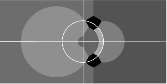
Figure 1: Different shades correspond to different fractional transformations chosen depending on the location of $z$ in the complex plane. The coordinate axes and the unit circle are drawn in white. Black indicates the corner cases where no transformation is effective.

7.2 Parameter limits

The $1/z$ and $1/(1-z)$ transformations involve a division by $\sin(\pi(b-a))$, and the $1-z$ and $1-1/z$ transformations involve a division by $\sin(\pi(c-a-b))$. Therefore, when $b-a$ or $c-a-b$ respectively is an integer, we compute $\lim_{\varepsilon\to 0}{}_{2}F_{1}(a+\varepsilon,b,c,z)$ using $\mathbb{C}[[\varepsilon]]/\langle\varepsilon^{2}\rangle$ arithmetic.

The limit computation can only be done automatically when $b-a$ (or $c-a-b$) is an exact integer. If, for example, $a,b$ are intervals representing $\pi,\pi+1$ and $b-a$ thus is a nonexact interval containing 1, the output would not be finite. To solve this problem, Arb allows the user to pass boolean flags as input to the ${}_{2}F_{1}$ function, indicating that $b-a$ or $c-a-b$ represent exact integers despite $a,b,c$ being inexact.

7.3 Corner case

When $z$ is near $e^{\pm\pi i/3}$, we use analytic continuation. The function $f(z)={}_{2}F_{1}(a,b,c,z_{0}+z)$ satisfies

$$f^{\prime\prime}(z)=-\frac{P_{1}(z)}{P_{2}(z)}f^{\prime}(z)-\frac{P_{0}(z)}{P_{2}(z)}f(z).$$ (11)

with $P_{2}(z)=(z+z_{0})(z+z_{0}-1)$, $P_{1}(z)=(a+b+1)(z+z_{0})-c$, $P_{0}(z)=ab$. It follows from (11) that the coefficients in the Taylor series $f(z)=\sum_{k=0}^{\infty}f_{[k]}z^{k}$ satisfy the second-order recurrence equation

$$R_{2}(k)f_{[k+2]}+R_{1}(k)f_{[k+1]}+R_{0}(k)f_{[k]}=0$$ (12)

with $R_{2}(k)=(k+1)(k+2)(z_{0}-1)z_{0}$, $R_{1}(k)=(k+1)(2k+a+b+1)z_{0}-(k+1)(k+c)$, $R_{0}(k)=(a+k)(b+k)$.

Knowing $f(0),f^{\prime}(0)$, we can compute $f(z),f^{\prime}(z)$ if $z$ is sufficiently small and $z_{0}\not\in\{0,1\}$, thanks to (12) and the truncation bound given below. We use the usual ${}_{2}F_{1}$ series at the origin, following by two analytic continuation steps

$$0\quad\to\quad 0.375\pm 0.625i\quad\to\quad 0.5\pm 0.8125i\quad\to\quad z.$$

This was found to be a good choice based on experiments. There is a tradeoff involved in choosing the evaluation points, since smaller steps yield faster local convergence.

Currently, BS and other reduced-complexity methods are not implemented for this Taylor series in Arb. At high precision, assuming that the parameters $a,b,c$ have short representations, it would be better to choose a finer path in which $z_{k}$ approaches the final evaluation point as $2^{-k}$, with BS to evaluate the Taylor series (this is known as the bit-burst method).

Though only used by default in the corner case, the user can invoke analytic continuation along an arbitrary path; for example, by crossing $(1,\infty)$, a non-principal branch can be computed.

A simple bound for the coefficients in the Taylor series is obtained using the Cauchy-Kovalevskaya majorant method, following [66].

Theorem 2.

If $f(z)=\sum_{k=0}^{\infty}f_{[k]}z^{k}$ satisfies (11) and $z_{0}\not\in\{0,1\}$, then for all $k\geq 0$, $|f_{[k]}|\leq A\binom{N+k}{k}\nu^{k}$ provided that

$$\nu\geq\max\left(\frac{1}{|z_{0}-1|},\frac{1}{|z_{0}|}\right),\quad M_{0}\geq 2\nu|ab|,\quad M_{1}\geq\nu(|a+b+1|+2|c|),$$ (13)

$$N \geq\frac{\max(\sqrt{2M_{0}},2M_{1})}{\nu},$$ (14)

$$A \geq\max\left(|f_{[0]}|,\frac{|f_{[1]}|}{\nu(N+1)}\right).$$ (15)

Proof.

Note that

$$\frac{1}{P_{2}(z)}=\frac{1}{z+z_{0}-1}-\frac{1}{z+z_{0}}=\sum_{k=0}^{\infty}\left(\frac{1}{(z_{0}-1)^{k+1}}-\frac{1}{z_{0}^{k+1}}\right)(-z)^{k}.$$

Accordingly, with $M_{0},M_{1},\nu$ as in (13),

$$\left|\left(-\frac{P_{i}(z)}{P_{2}(z)}\right)_{[k]}\right|\leq M_{i}\nu^{k}=\left(\frac{M_{i}}{1-\nu z}\right)_{[k]},\quad i=0,1.$$

In other words, (11) is majorized by $g^{\prime\prime}(z)=\frac{M_{1}}{1-\nu z}g^{\prime}(z)+\frac{M_{0}}{1-\nu z}g(z).$ Using (14) in turn gives the majorizing differential equation

$$h^{\prime\prime}(z)=\frac{N+1}{2}\left(\frac{\nu}{1-\nu z}\right)h^{\prime}(z)+\frac{(N+1)N}{2}\left(\frac{\nu}{1-\nu z}\right)^{2}h(z).$$ (16)

The simple solution $h(z)=A(1-\nu z)^{-N}$ of (16) now provides the bound $|f_{[k]}|\leq h_{[k]}=A\binom{N+k}{k}\nu^{k}$ with $A$ chosen as in (15) for the initial values. ∎

Note that the bound is a hypergeometric sequence, indeed $h(z)=A\,{}_{1}F_{0}(N,\nu z)$, so the tail of the Taylor series is easily bounded as in subsection 4.1.

A different method to evaluate ${}_{2}F_{1}$ in the corner case is used in Mathematica, Maxima, mpmath and perhaps others [25, 68]. No error bounds have been published for that method; we encourage further investigation.

7.4 Numerical stability

Unlike the confluent hypergeometric functions, cancellation is not a problem for any $z$ as long as the parameters are small. With small complex parameters and 64-bit precision, about 5-10 bits are lost on most of the domain, up to about 25 bits in the black regions of Figure 1, so even machine precision interval arithmetic would be adequate for many applications. However, cancellation does become a problem with large parameters (e.g. for orthogonal polynomials of high degree). The current implementation could be improved for some cases by using argument transformations and recurrence relations to minimize cancellation.

7.5 Higher orders

The functions ${}_{3}F_{2}$, ${}_{4}F_{3}$, etc. have a $1/z$ transformation analogous to (10), but no other such formulas for generic parameters [21, 16.8]. We could cover $|z|\gg 1$ by evaluating ${}_{p}F_{q}$-series directly, but other methods are needed on the annulus surrounding the unit circle. Convergence accelerations schemes such as [69, 7, 56] can be effective, but the D-finite analytic continuation approach (with the singular expansion at $z=1$) is likely better since effective error bounds are known and since complexity-reduction techniques apply. A study remains to be done.

We note that an important special function related to ${}_{n+1}F_{n}$, the polylogarithm $\operatorname{Li}_{s}(z)$, is implemented for general complex $s,z$ in Arb, using direct series for $|z|\ll 1$ and the Hurwitz zeta function otherwise [35]. Also $s$-derivatives are supported.

8 Benchmarks

We compare Arb (git version as of June 2016) to software for specific functions, and to Mathematica 10.4 which supports arbitrary-precision evaluation of generalized hypergeometric functions. Tests were run on an Intel i5-4300U CPU except Mathematica which was run on an Intel i7-2600 (about 20% faster). All timing measurements have been rounded to two digits.

8.1 Note on Mathematica

We compare to Mathematica since it generally appears faster than Maple and mpmath. It also attempts to track numerical errors, using a form of significance arithmetic [59]. With f=Hypergeometric1F1, the commands f[-1000,1,N[1,30]], N[f[-1000,1,1]], and N[f[-1000,1,1],30] give $0.155$, $0.154769$, and $0.154769339118406535633854462041$, where all results show loss of significance being tracked correctly. Note that N[..., d] attempts to produce $d$ significant digits by adaptively using a higher internal precision. For comparison, at 64 and 128 bits, Arb produces $[\pm 5.51\cdot 10^{6}]$ and $[0.154769339118\pm 9.35\cdot 10^{-13}]$.

Unfortunately, Mathematica’s heuristic error tracking is unreliable. For example, f[-1000,1,1.0], produces $-1.86254761018\cdot 10^{9}$ without any hint that the result is wrong. The input 1.0 designates a machine-precision number, which in Mathematica is distinct from an arbitrary-precision number, potentially disabling error tracking in favor of speed (one of many pitfalls that the user must be aware of). However, even arbitrary-precision results obtained from exact input cannot be trusted:

In[1]:= a=8106479329266893*2^-53; b=1/2 + 3900231685776981*2^-52 I;
In[2]:= f=Hypergeometric2F1[1,a,2,b];
In[3]:= Print[N[f,16]]; Print[N[f,20]]; Print[N[f,30]];
0.9326292893367381 + 0.4752101514062250 I
0.93263356923938324111 + 0.47520053858749520341 I
0.932633569241997940484079782656 + 0.475200538581622492469565624396 I
In[4]:= f=Log[-Re[Hypergeometric2F1[500I,-500I,-500+10(-500)I,3/4]]];
In[5]:= $MaxExtraPrecision=10^4; Print[{N[f,100],N[f,200],N[f,300]}//N];
{2697.18, 2697.18, 2003.57}

As we see, even comparing answers computed at two levels of precision (100 and 200 digits) for consistency is not reliable. Like with most numerical software (this is not a critique of Mathematica in particular), Mathematica users must rely on external knowledge to divine whether results are likely to be correct.

8.2 Double precision

Pearson gives a list of 40 inputs $(a,b,z)$ for ${}_{1}F_{1}$ and 30 inputs $(a,b,c,z)$ for ${}_{2}F_{1}$, chosen to exercise different evaluation regimes in IEEE 754 double precision implementations [51, 52]. We also test $U(a,b,z)$ with the ${}_{1}F_{1}$ inputs and the Legendre function $Q_{a}^{c}(1-2z)$ with the ${}_{2}F_{1}$ inputs (with argument $1-2z$, it is equivalent to a linear combination of two ${}_{2}F_{1}$’s of argument $z$).

	Code	Average	Median	Accuracy
${}_{1}F_{1}$	SciPy	2.7	0.76	18 good, 4 fair, 4 poor, 5 wrong, 2 NaN, 7 skipped
${}_{2}F_{1}$	SciPy	24	0.56	18 good, 1 fair, 1 poor, 3 wrong, 1 NaN, 6 skipped
${}_{2}F_{1}$	Michel & S.	7.7	2.1	22 good, 1 poor, 6 wrong, 1 NaN
${}_{1}F_{1}$	MMA (m)	1100	29	34 good, 2 poor, 4 wrong, 2 no significant digits out
${}_{2}F_{1}$	MMA (m)	30000	72	29 good, 1 fair
$U$	MMA (m)	4400	190	28 good, 4 fair, 2 wrong, 6 no significant digits out
$Q$	MMA (m)	4300	61	21 good, 3 fair, 2 poor, 1 wrong, 3 NaN
${}_{1}F_{1}$	MMA (a)	2100	170	39 good, 1 not good as claimed (actual error $2^{-40}$)
${}_{2}F_{1}$	MMA (a)	37000	540	30 good ($2^{-53}$)
$U$	MMA (a)	25000	340	38 good, 2 not as claimed ($2^{-40},2^{-45}$)
$Q$	MMA (a)	8300	780	28 good, 1 not as claimed ($2^{-25}$), 1 wrong
${}_{1}F_{1}$	Arb	200	32	40 good (correct rounding)
${}_{2}F_{1}$	Arb	930	160	30 good (correct rounding)
$U$	Arb	2000	93	40 good (correct rounding)
$Q$	Arb	3000	210	30 good ($2^{-53}$)

Table 3: Time (in microseconds) per function evaluation, averaged over the 30 or 40 inputs, and resulting accuracy. MMA is Mathematica, with (m) machine precision and (a) arbitrary-precision arithmetic. With SciPy, Michel & S. and MMA (m), we deem a result with relative error at most $2^{-40}$ good, $2^{-20}$ fair, $2^{-1}$ poor, otherwise wrong. With MMA (a), good is $<2^{-50}$.

With Arb, we measure the time to compute certified correctly rounded 53-bit floating-point values, except for the function $Q$ where we compute the values to a certified relative error of $2^{-53}$ before rounding (in the current version, some exact outputs for this function are not recognized, so the correct-rounding loop would not terminate). We interpret all inputs as double precision constants rather than real or complex numbers that would need to be enclosed by intervals. For example, $0.1=3602879701896397\cdot 2^{-55}$, $e^{i\pi/3}=2^{-1}+3900231685776981\cdot 2^{-52}i$. This has no real impact on this particular benchmark, but it is simpler and demonstrates Arb as a black box to implement floating-point functions.

For ${}_{2}F_{1}$, we compare with the double precision C++ implementation by Michel and Stoitsov [48]. We also compare with the Fortran-based ${}_{1}F_{1}$ and ${}_{2}F_{1}$ implementations in SciPy [36], which only support inputs with real parameters.

We test Mathematica in two ways: with machine precision numbers as input, and using its arbitrary-precision arithmetic to attempt to get 16 significant digits. N[] does not work well on this benchmark, because Mathematica gets stuck expanding huge symbolic expressions when some of the inputs are given exactly (N[] also evaluates some of those resulting expressions incorrectly), so we implemented a precision-increasing loop like the one used with Arb instead.

Since some test cases take much longer than others, we report both the average and the median time for a function evaluation with each implementation.

The libraries using pure machine arithmetic are fast, but output wrong values in several cases. Mathematica with machine-precision input is only slightly more reliable. With arbitrary-precision numbers, Mathematica’s significance arithmetic computes most values correctly, but the output is not always correct to the 16 digits Mathematica claims. One case, $Q_{500}^{500}(11/5)$, is completely wrong. Mathematica’s ${}_{2}F_{1}$ passes, but as noted earlier, would fail with the built-in N[]. Arb is comparable to Mathematica’s machine precision in median speed (around $10^{4}$ function evaluations per second), and has better worst-case speed, with none of the wrong results.

8.3 Complex Bessel functions

Kodama [38] has implemented the functions $J_{\nu}(z),Y_{\nu}(z)$ and $H^{(1),(2)}_{\nu}(z)=J_{\nu}\pm iY_{\nu}(z)$ for complex $\nu,z$ accurately (but without formal error bounds) in Fortran. Single, double and extended (targeting $\approx 70$-bit accuracy) precision are supported. Kodama’s self-test program evaluates all four functions with parameter $\nu$ and $\nu+1$ for 2401 pairs $\nu,z$ with real and imaginary parts between $\pm 60$, making 19 208 total function calls. Timings are shown in Table 4.

Code	Time	4-in-1	Accuracy
Kodama, 53-bit	4.7		19208 good ($\approx 2^{-45}$) according to self-test
Kodama, $\approx$ 80-bit	270		19208 good ($\approx 2^{-68}$) according to self-test
MMA (machine)	75		14519 good, 607 fair, 256 poor, 3826 wrong
MMA (N[], 53-bit)	270		17484 good, 2 fair, 273 poor, 1449 wrong
MMA (N[], 113-bit)	340		18128 good, 206 fair, 187 poor, 687 wrong
Arb (53-bit)	10	5.1	19208 good (correct rounding)
Arb (113-bit)	11	5.9	19208 good (correct rounding)

Table 4: Time (in seconds) to compute the 19 208 Bessel function values in Kodama’s test. The good/fair/poor/wrong thresholds are $2^{-40}$ (53-bit) or $2^{-100}$ (113-bit) / $2^{-20}$ / $2^{-1}$.

We compiled Kodama’s code with GNU Fortran 4.8.4, which uses a quad precision (113-bit or 34-digit) type for extended precision. We use Arb to compute the functions on the same inputs, to double and quad precision with certified correct rounding of both the real and imaginary parts. In the 4-in-1 column for Arb, we time computing the four values $J,Y,H^{(1)},H^{(2)}$ simultaneously rather than with separate calls, still with correct rounding for each function. Surprisingly, our implementation is competitive with Kodama’s double precision code, despite ensuring correct rounding. There is a very small penalty going from double to quad precision, due to the fact that a working precision of 200-400 bits is used in the first place for many of the inputs.

We also test Mathematica in three ways: with machine precision input, and with exact input using N[...,16] or N[...,34]. Mathematica computes many values incorrectly. For example, with $\nu=-53.9-53.4i,z=-54.7+17.61i$, the three evaluations of the HankelH1 function give three different results

$$\begin{array}[]{c}H^{(1)}_{\nu}(z)=1.30261\cdot 10^{-34}-4.49948\cdot 10^{-35}i,\\ H^{(1)}_{\nu}(z)=-1.18418492459404\cdot 10^{-32}+2.805568990224272\cdot 10^{-31}i,\\ H^{(1)}_{\nu}(z)=-3.893447525697409211107221229269630\cdot 10^{-25}+\\ 6.133044639987209608932345865755910\cdot 10^{-25}i\end{array}$$

while the correct value is about $1.65\cdot 10^{-27}+2.28\cdot 10^{-27}i$.

8.4 High precision

Table 5 shows the time to compute Bessel functions for small $\nu$ and $z$, varying the precision and the type of the inputs. In A, both $\nu$ and $z$ have few bits, and Arb uses BS. In B, $\nu$ has few bits but $z$ has full precision, and RS is used. In C, both $\nu$ and $z$ have full precision, and FME is used. Since much of the time in C is spent computing $\Gamma(\pi+1)$, D tests $J_{\pi}(\pi)$ without this factor. E and F involve computing the parameter derivatives of two ${}_{0}F_{1}$ functions with $\mathbb{C}[[x]]/\langle x^{2}\rangle$ arithmetic to produce $K_{3}(z)$, respectively using BS and RS.

In all cases, complexity-reducing methods give a notable speedup at high precision. Only real values are tested; complex numbers (when of similar “difficulty” on the function’s domain) usually increase running times uniformly by a factor 2–4.

	Mathematica					Arb
	10	100	1000	10 000	100 000	10	100	1000	10 000	100 000
A: $J_{3}(3.25)$	24	48	320	9200	590 000	6	27	140	1600	26 000
B: $J_{3}(\pi)$	23	56	800	110 000	17 000 000	7	28	320	14 000	960 000
C: $J_{\pi}(\pi)$	58	220	34 000	8 500 000		12	91	2800	270 000	44 000 000
D: ${}_{0}F_{1}(\pi\!+\!1,-\tfrac{\pi^{2}}{4})\!$	26	84	1800	350 000	61 000 000	7	49	1500	93 000	14 000 000
E: $K_{3}(3.25)$	68	160	1700	140 000	19 000 000	40	150	1300	20 000	500 000
F: $K_{3}(\pi)$	69	160	2600	350 000	52 000 000	43	170	1900	67 000	4 100 000

Table 5: Time (in microseconds) to compute easy values to 10, 100, 1000, 10 000 and 100 000 digits. Note: in case C, Arb takes 360 s the first time at $10^{5}$ digits, due to precomputing Bernoulli numbers.

8.5 Large parameters and argument

Table 6 compares global performance of confluent hypergeometric functions. Each function is evaluated at 61 exponentially spaced arguments $z_{k}=\pi 10^{k/10},0\leq k\leq 60$ for varying precision or parameter magnitudes, covering the convergent, asymptotic and transition regimes.

We include timings for MPFR, which implements $J_{N}(z)$ for $N\in\mathbb{Z},z\in\mathbb{R}$ in floating-point arithmetic with correct rounding. At low precision, Arb computes $J_{N}(z)$ about 2-3 times slower than MPFR. This factor is explained by Arb’s lack of automatic compensation for precision loss, the ${}_{0}F_{1}(b,z)$ series evaluation not being optimized specifically for $b\in\mathbb{Z},z\in\mathbb{R}$, and complex arithmetic being used for the asymptotic expansion, all of which could be addressed in the future.

Figure 2 shows a more detailed view of test cases A (MPFR, Arb) and G (Mathematica, Arb). The evaluation time peaks in the transition region between the convergent and asymptotic series. Approaching the peak, the time increases smoothly as more terms are required. With Arb, sudden jumps are visible where the precision is doubled. By tuning the implementation of $J_{0}(z)$, the jumps could be smoothed out. In test case B (not plotted), there is no cancellation, and no such jumps occur. Mathematica is slow with large parameters (we get more than a factor $10^{5}$ speedup), likely because it is conservative about using the asymptotic expansion. Since Arb computes a rigorous error bound, the asymptotic expansion can safely be used aggressively.

	Mathematica				Arb
Function $\backslash$ $N$	10	100	1000	10000	10	100	1000	10000
A: $J_{0}(z)$	0.0039	0.020	3.0	4700	0.00097	0.0064	0.12	7.7
B: $I_{0}(z)$	0.0032	0.012	1.5	2000	0.00081	0.0042	0.067	3.4
C: $J_{0}(\omega z)$	0.0099	0.072	16	36000	0.0014	0.0069	0.16	11
D: $K_{0}(z)$	0.0037	0.028	4.2	5900	0.0018	0.020	0.47	28
E: $J_{N}(z)$	0.0038	0.0073	0.31	46	0.0010	0.0054	0.13	2.7
F: $J_{Ni}(z)$	0.0089	28	$>10^{5}$	$>10^{5}$	0.0017	0.0096	0.14	10
G: ${}_{1}F_{1}(Ni,1+i,\omega z)$	0.13	15	15000	$>10^{5}$	0.0082	0.061	1.3	82
	MPFR
A: $J_{0}(z)$	0.00057	0.0030	0.24	42
E: $J_{N}(z)$	0.00078	0.0021	0.039	2.7

Table 6: Time in seconds to evaluate the functions on 61 exponentially spaced points from $\pi$ to $10^{6}\pi$. In A–D, the function is computed to $N$ digits, $N=10,10^{2},10^{3},10^{4}$. In E–G, the function is computed to 10 digits, with $N$ or $Ni$ ($i=\sqrt{-1}$) as a parameter. Here, $\omega=e^{\pi i/3}$.

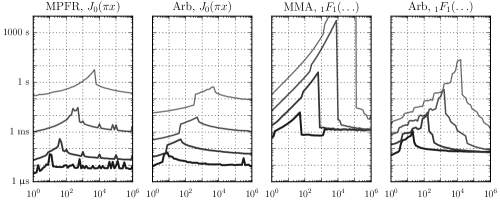
Figure 2: Time as a function of $x$ to evaluate $J_{0}(\pi x)$ to $N$ digits and ${}_{1}F_{1}(Ni,1+i,e^{\pi i/3}\pi x)$ to 10 digits, for $N=10^{1},10^{2},10^{3},10^{4}$ (from bottom to top).

8.6 Airy function zeros

Arb includes code for rigorously computing all the zeros of a real analytic functions on a finite interval. Sign tests and interval bisection are used to find low-precision isolating intervals for all zeros, and then as an optional stage rigorous Newton iteration is used to refine the zeros to high precision.

Arb takes 0.42 s to isolate the 6710 zeros of $\operatorname{Ai}(z)$ on the interval $[-1000,0]$ (performing 67 630 function evaluations), 1.3 s to isolate and refine the zeros to 16-digit accuracy (181 710 evaluations), and 23 s to isolate and refine the zeros to 1000-digit accuracy (221 960 evaluations). Mathematica’s built-in AiryAiZero takes 2.4 s for machine or 16-digit accuracy and 264 s for 1000-digit accuracy.

Note that the Arb zero-finding only uses interval evaluation of $\operatorname{Ai}(z)$ and its derivatives; no a priori knowledge about the distribution of zeros is exploited.

8.7 Parameter derivatives

We compute $\partial_{\nu}^{n}J_{\nu}(z)|_{\nu=1,z=\pi}$ to 100 digits, showing timings in Table 7. Mathematica’s N[] scales very poorly. We also include timings with Maple 2016 (on the same machine as Mathematica), using fdiff which implements numerical differentiation. This performs better, but the automatic differentiation in Arb is far superior. In fact, Maple automatically uses parallel computation (8 cores), and its total CPU time is several times higher than the wall time shown in Table 7.

Code \$\;n$	1	2	5	10	100	1000	10000
Mathematica	0.12	0.20	2600
Maple (8 cores)	0.024	0.039	4.3	35	$>1$ h
Arb	0.000088	0.00015	0.00031	0.00058	0.017	6.6	1400

Table 7: Time (in seconds) to compute parameter $n$-th derivatives.

9 Conclusion

We have demonstrated that it is practical to guarantee rigorous error bounds for arbitrary-precision evaluation of a wide range of special functions, even with complex parameters. Interval arithmetic is seen to work very well, and the methods presented here could be exploited in other software. The implementation in Arb is already being used in applications, but it is a work in progress, and many details could still be optimized. For example, recurrence relations and alternative evaluation formulas could be incorporated to reduce cancellation, and internal parameters such as the number of terms and the working precision could be chosen more intelligently. More fundamentally, we have not addressed the following important issues:

• Rigorous error bounds for asymptotic expansions of the generalized hypergeometric function ${}_{p}F_{q}$ in cases not covered by the $U$-function.

• Efficient support for exponentially large parameter values (e.g. $|a|\gg 10^{4}$, say in time polynomial in $\log|a|$ rather than in $|a|$), presumably via asymptotic expansions with respect to the parameters.

• Methods to compute tight bounds when given wide intervals as input, apart from the simple cases where derivatives and functional equations can be used.

• Using machine arithmetic where possible to speed up low-precision evaluation.

• Formal code verification, to eliminate bugs that may slip past both human review and randomized testing.

References

- [1] M. Abramowitz and I. A. Stegun, Handbook of Mathematical Functions with Formulas, Graphs, and Mathematical Tables, Dover, New York, 1964.
- [2] D. H. Bailey, MPFUN2015: A thread-safe arbitrary precision computation package, (2015).
- [3] D. H. Bailey and J. M. Borwein, High-precision arithmetic in mathematical physics, Mathematics, 3 (2015), pp. 337–367.
- [4] D. H. Bailey, J. M. Borwein, and R. E. Crandall, Integrals of the Ising class, Journal of Physics A: Mathematical and General, 39 (2006), pp. 12271–12302, http://dx.doi.org/10.1088/0305-4470/39/40/001.
- [5] D. J. Bernstein, Fast multiplication and its applications, Algorithmic Number Theory, 44 (2008), pp. 325–384.
- [6] R. Bloemen, Even faster calculation! https://web.archive.org/web/20141101133659/http://xn--2-umb.com/09/11/even-faster-zeta-calculation, 2009.
- [7] A. I. Bogolubsky and S. L. Skorokhodov, Fast evaluation of the hypergeometric function at the singular point by means of the Hurwitz zeta function , Programming and Computer Software, 32 (2006), pp. 145–153.
- [8] A. R. Booker, A. Strömbergsson, and A. Venkatesh, Effective computation of Maass cusp forms, International Mathematics Research Notices, (2006).
- [9] J. M. Borwein, D. M. Bradley, and R. E. Crandall, Computational strategies for the Riemann zeta function, Journal of Computational and Applied Mathematics, 121 (2000), pp. 247–296.
- [10] J. M. Borwein and I. J. Zucker, Fast evaluation of the gamma function for small rational fractions using complete elliptic integrals of the first kind, IMA Journal of Numerical Analysis, 12 (1992), pp. 519–526.
- [11] P. Borwein, An efficient algorithm for the Riemann zeta function, Canadian Mathematical Society Conference Proceedings, 27 (2000), pp. 29–34.
- [12] P. B. Borwein, Reduced complexity evaluation of hypergeometric functions, Journal of Approximation Theory, 50 (1987).
- [13] A. Bostan, P. Gaudry, and E. Schost, Linear recurrences with polynomial coefficients and application to integer factorization and Cartier-Manin operator, SIAM Journal on Computing, 36 (2007), pp. 1777–1806.
- [14] R. P. Brent, The complexity of multiple-precision arithmetic, The Complexity of Computational Problem Solving, (1976), pp. 126–165.
- [15] R. P. Brent and F. Johansson, A bound for the error term in the Brent-McMillan algorithm, Mathematics of Computation, 84 (2015), pp. 2351–2359.
- [16] R. P. Brent and P. Zimmermann, Modern Computer Arithmetic, Cambridge University Press, 2011.
- [17] S. Chevillard and M. Mezzarobba, Multiple-precision evaluation of the Airy Ai function with reduced cancellation, in 21st IEEE Symposium on Computer Arithmetic, ARITH21, 2013, pp. 175–182, http://dx.doi.org/10.1109/ARITH.2013.33.
- [18] D. V. Chudnovsky and G. V. Chudnovsky, Approximations and complex multiplication according to Ramanujan, in Ramanujan Revisited, Academic Press, 1988, pp. 375–472.
- [19] D. V. Chudnovsky and G. V. Chudnovsky, Computer algebra in the service of mathematical physics and number theory, Computers in mathematics, 125 (1990), p. 109.
- [20] M. Colman, A. Cuyt, and J. V. Deun, Validated computation of certain hypergeometric functions, ACM Transactions on Mathematical Software, 38 (2011).
- [21] NIST Digital Library of Mathematical Functions. http://dlmf.nist.gov/, Release 1.0.11 of 2016-06-08, http://dlmf.nist.gov/. Online companion to [50].
- [22] Z. Du, Guaranteed precision for transcendental and algebraic computation made easy, PhD thesis, New York University, New York, NY, 2006.
- [23] Z. Du, M. Eleftheriou, J. E. Moreira, and C. Yap, Hypergeometric functions in exact geometric computation, Electronic Notes in Theoretical Computer Science, 66 (2002), pp. 53–64.
- [24] A. Enge, P. Théveny, and P. Zimmermann, MPC: a library for multiprecision complex arithmetic with exact rounding. http://multiprecision.org/, 2011.
- [25] R. Fateman, [[Maxima] numerical evaluation of 2F1] from RW Gosper. http://www.math.utexas.edu/pipermail/maxima/2006/000126.html. Post to the Maxima mailing list.
- [26] S. Fillebrown, Faster computation of Bernoulli numbers, Journal of Algorithms, 13 (1992), pp. 431–445.
- [27] P. Flajolet and I. Vardi, Zeta function expansions of classical constants, (1996).
- [28] L. Fousse, G. Hanrot, V. Lefèvre, P. Pélissier, and P. Zimmermann, MPFR: A multiple-precision binary floating-point library with correct rounding, ACM Transactions on Mathematical Software, 33 (2007), pp. 13:1–13:15. http://mpfr.org.
- [29] B. Haible and T. Papanikolaou, Fast multiprecision evaluation of series of rational numbers, in Algorithmic Number Theory: Third International Symposium, ANTS-III, J. P. Buhler, ed., Springer, 1998, pp. 338–350, http://dx.doi.org/10.1007/BFb0054873.
- [30] F. Johansson, Arb: a C library for ball arithmetic, ACM Communications in Computer Algebra, 47 (2013), pp. 166–169, http://dx.doi.org/10.1145/2576802.2576828.
- [31] F. Johansson, Evaluating parametric holonomic sequences using rectangular splitting, in Proceedings of the 39th International Symposium on Symbolic and Algebraic Computation, ISSAC ’14, ACM, 2014, pp. 256–263, http://dx.doi.org/10.1145/2608628.2608629.
- [32] F. Johansson, Fast and rigorous computation of special functions to high precision, PhD thesis, RISC, Johannes Kepler University, Linz, 2014. http://fredrikj.net/thesis/.
- [33] F. Johansson, Efficient implementation of elementary functions in the medium-precision range, in 22nd IEEE Symposium on Computer Arithmetic, ARITH22, 2015, pp. 83–89, http://dx.doi.org/10.1109/ARITH.2015.16.
- [34] F. Johansson, mpmath: a Python library for arbitrary-precision floating-point arithmetic. http://mpmath.org, 2015.
- [35] F. Johansson, Rigorous high-precision computation of the Hurwitz zeta function and its derivatives, Numerical Algorithms, 69 (2015), pp. 253–270, http://dx.doi.org/10.1007/s11075-014-9893-1.
- [36] E. Jones, T. Oliphant, P. Peterson, et al., SciPy: Open source scientific tools for Python. http://www.scipy.org/, 2001–.
- [37] E. A. Karatsuba, Fast evaluation of the Hurwitz zeta function and Dirichlet -series, Problems of Information Transmission, 34 (1998).
- [38] M. Kodama, Algorithm 912: A module for calculating cylindrical functions of complex order and complex argument, ACM Transactions on Mathematical Software, 37 (2011), pp. 1–25.
- [39] S. Köhler and M. Ziegler, On the stability of fast polynomial arithmetic, in Proceedings of the 8th Conference on Real Numbers and Computers, Santiago de Compostela, Spain, 2008.
- [40] K. Kuhlman, Unconfined: command-line parallel unconfined aquifer test simulator. https://github.com/klkuhlm/unconfined, 2015.
- [41] C. Lanczos, A precision approximation of the gamma function, SIAM Journal on Numerical Analysis, 1 (1964), pp. 86–96.
- [42] Maplesoft, Maple. http://www.maplesoft.com/documentation_center/, 2016.
- [43] Maxima authors, Maxima, a computer algebra system. http://maxima.sourceforge.net/, 2015.
- [44] M. Mezzarobba, Rigorous multiple-precision evaluation of D-finite functions in Sage, in Mathematical Software – ICMS 2016, 5th International Congress, Lecture Notes in Computer Science 9725, G. M. Greuel, T. Koch, P. Paule, and A. Sommese, eds., Springer. To appear.
- [45] M. Mezzarobba, NumGfun: a package for numerical and analytic computation with D-finite functions, in Proceedings of ISSAC’10, 2010, pp. 139–146.
- [46] M. Mezzarobba, Autour de l’évaluation numérique des fonctions D-finies, thèse de doctorat, Ecole polytechnique, Nov. 2011.
- [47] M. Mezzarobba and B. Salvy, Effective bounds for P-recursive sequences, Journal of Symbolic Computation, 45 (2010), pp. 1075–1096, http://dx.doi.org/10.1016/j.jsc.2010.06.024, http://arxiv.org/abs/0904.2452.
- [48] N. Michel and M. V. Stoitsov, Fast computation of the Gauss hypergeometric function with all its parameters complex with application to the Pöschl–Teller–Ginocchio potential wave functions, Computer Physics Communications, 178 (2008), pp. 535–551.
- [49] F. W. J. Olver, Asymptotics and Special Functions, A K Peters, Wellesley, MA, 1997.
- [50] F. W. J. Olver, D. W. Lozier, R. F. Boisvert, and C. W. Clark, NIST Handbook of Mathematical Functions, Cambridge University Press, New York, 2010.
- [51] J. Pearson, Computation of hypergeometric functions, master’s thesis, University of Oxford, 2009.
- [52] J. W. Pearson, S. Olver, and M. A. Porter, Numerical methods for the computation of the confluent and Gauss hypergeometric functions, arXiv:1407.7786, http://arxiv.org/abs/1407.7786, (2014).
- [53] N. Revol and F. Rouillier, Motivations for an arbitrary precision interval arithmetic library and the MPFI library, Reliable Computing, 11 (2005), pp. 275–290. http://perso.ens-lyon.fr/nathalie.revol/software.html.
- [54] Sage developers, SageMath, the Sage Mathematics Software System (Version 7.2.0), 2016. http://www.sagemath.org.
- [55] T. Schmelzer and L. N. Trefethen, Computing the gamma function using contour integrals and rational approximations, SIAM Journal on Numerical Analysis, 45 (2007), pp. 558–571.
- [56] S. L. Skorokhodov, A method for computing the generalized hypergeometric function in terms of the Riemann zeta function, Computational Mathematics and Mathematical Physics, 45 (2005), pp. 574–586.
- [57] D. M. Smith, Efficient multiple-precision evaluation of elementary functions, Mathematics of Computation, 52 (1989), pp. 131–134.
- [58] D. M. Smith, Algorithm: Fortran 90 software for floating-point multiple precision arithmetic, gamma and related functions, Transactions on Mathematical Software, 27 (2001), pp. 377–387.
- [59] M. Sofroniou and G. Spaletta, Precise numerical computation, Journal of Logic and Algebraic Programming, 64 (2005), pp. 113–134.
- [60] J. L. Spouge, Computation of the gamma, digamma, and trigamma functions, SIAM Journal on Numerical Analysis, 31 (1994), pp. 931–944.
- [61] T. P. Stefański, Electromagnetic problems requiring high-precision computations, IEEE Antennas and Propagation Magazine, 55 (2013), pp. 344–353, http://dx.doi.org/10.1109/MAP.2013.6529388.
- [62] The MPFR team, The MPFR library: algorithms and proofs. http://www.mpfr.org/algo.html. Retrieved 2013.
- [63] The PARI group, PARI/GP, Bordeaux. http://pari.math.u-bordeaux.fr.
- [64] W. Tucker, Validated numerics: a short introduction to rigorous computations, Princeton University Press, 2011.
- [65] J. van der Hoeven, Fast evaluation of holonomic functions, Theoretical Computer Science, 210 (1999), pp. 199–215.
- [66] J. van der Hoeven, Fast evaluation of holonomic functions near and in regular singularities, Journal of Symbolic Computation, 31 (2001), pp. 717–743.
- [67] J. van der Hoeven, Ball arithmetic, tech. report, HAL, 2009. http://hal.archives-ouvertes.fr/hal-00432152/fr/.
- [68] A. Vogt, Computing the hypergeometric function 2F1 using a recipe of Gosper. http://www.axelvogt.de/axalom/hyp2F1/hypergeometric_2F1_using_a_recipe_of_Gosper.mws.pdf.
- [69] J. L. Willis, Acceleration of generalized hypergeometric functions through precise remainder asymptotics, Numerical Algorithms, 59 (2012), pp. 447–485.
- [70] Wolfram Research, The Wolfram Functions Site. http://functions.wolfram.com/.
- [71] Wolfram Research, Mathematica. http://wolfram.com, 2016.
- [72] N. Yamamoto and N. Matsuda, Validated computation of Bessel functions, in 2005 International Symposium on Nonlinear Theory and its Applications (NOLTA2005). http://www.ieice.org/proceedings/NOLTA2005/HTMLS/paper/715A.pdf.
- [73] M. Ziegler, Fast (multi-)evaluation of linearly recurrent sequences: Improvements and applications, (2005). http://arxiv.org/abs/cs/0511033.