From a quasimolecular band insulator to a relativistic Mott insulator in $t_{2g}^{5}$ systems with a honeycomb lattice structure

Abstract

The $t_{2g}$ orbitals of an edge-shared transition-metal oxide with a honeycomb lattice structure form dispersionless electronic bands when only hopping mediated by the edge-sharing oxygens is accessible. This is due to the formation of isolated quasimolecular orbitals (QMOs) in each hexagon, introduced recently by Mazin et al. [Phys. Rev. Lett. 109, 197201 (2012)], which stabilizes a band insulating phase for $t_{2g}^{5}$ systems. However, with help of the exact diagonalization method to treat the electron kinetics and correlations on an equal footing, we find that the QMOs are fragile against not only the spin-orbit coupling (SOC) but also the Coulomb repulsion. We show that the electronic phase of $t_{2g}^{5}$ systems can vary from a quasimolecular band insulator to a relativistic $J_{\rm eff}=1/2$ Mott insulator with increasing the SOC as well as the Coulomb repulsion. The different electronic phases manifest themselves in electronic excitations observed in optical conductivity and resonant inelastic x-ray scattering. Based on our calculations, we assert that the currently known Ru³⁺- and Ir⁴⁺-based honeycomb systems are far from the quasimolecular band insulator but rather the relativistic Mott insulator.

Introduction — Physical properties of $4d$ and $5d$ transition metal (TM) compounds with nominally less than six $d$ electrons are determined by the $t_{2g}$ manifold because of a strong cubic crystal field. A strong spin-orbit coupling (SOC) causes $t_{2g}$ orbitals split into effective total angular momenta $j_{\rm eff}=1/2$ and $3/2$. The relativistic electronic feature in these TM compounds has drawn much attraction recently as exotic electronic, magnetic, and topological phases have been expected, including $J_{\rm eff}=1/2$ Mott insulator BJKim2008 ; BJKim2009 ; Jackeli2009 ; Watanabe2010 ; Martins2011 , superconductivity Wang2011 ; Watanabe2013 , topological insulator Pesin2010 ; Yang2010 , Weyl semimetal Krempa2012 ; AGo2012 , and spin liquid Okamoto2007 ; Singh2013 . Among them, the research on $t_{2g}^{5}$ systems forming a honeycomb lattice structure with edge-sharing ligands has been triggered by the possibility of a nontrivial topological phase Shitade2009 ; CHKim2012 or a Kitaev-type spin liquid Chaloupka2010 ; Jiang2011 ; Reuther2011 , attributed to their unique hopping geometry. However, the existing compounds such as Na₂IrO₃ Singh2010 ; Liu2011 ; Choi2012 ; Ye2012 , Li₂IrO₃ Singh2012 , Li₂RhO₃ Luo2013 , and $\alpha$-RuCl₃ Sears2015 ; Majumder2015 ; Johnson2015 , have been turned out to be magnetic insulators with a long-range antiferromagnetic (AFM) or glassy-spin order.

In order to understand the electronic and magnetic structures of these compounds with $t_{2g}^{5}$ configuration, two distinct points of view, i.e., Mott- and Slater-type pictures, have been proposed. In the Mott picture, the Coulomb repulsion opens the gap of the relativistic $j_{\rm eff}=1/2$ based band and the superexchange interaction between the relativistic isospins stabilizes the AFM order Comin2012 ; Gretarsson2013 ; Sohn2013 ; BHKim2014 ; Plumb2014 ; HSKim2015 . This strong coupling approach can successfully elucidate the observed excitations in the optical conductivity (OC) and resonant inelastic x-ray scattering (RIXS) for Na₂IrO₃ BHKim2014 . However, there has been still debate on the origin of the zigzag AFM order in Na₂IrO₃ Kimchi2011 ; Chaloupka2013 . In contrast, the Slater picture focuses on the itinerant nature of $t_{2g}$ bands and treats the Coulomb interactions perturbatively. This weak coupling approach naturally explains the zigzag AFM order with a concomitantly induced band gap Mazin2012 ; Mazin2013 ; Foyevtsova2013 ; HJKim2014 . However, it is difficult to fully describe the observed excitations in the OC and RIXS for Na₂IrO₃ Li2015 ; MJKim2016 ; Igarashi2015 . Because the hopping integral, Coulomb repulsion, and SOC are of similar energy scale, either of these two opposite pictures cannot be ruled out.

As the electron hoppings between the adjacent TMs via the two edge-sharing ligands are highly orbital dependent Supp , the electron motion is confined within a single hexagon formed by six TMs. This has led to the notion of the quasimolecular orbital (QMO) formation Mazin2012 , where each $t_{2g}$ orbital of a TM participates in the formation of QMO at one of the three different hexagons around the TM. Therefore, when the SOC and Coulomb repulsion are both small, the ground state for $t_{2g}^{5}$ systems is a band insulator with a strong QMO character. However, when the SOC is strong, the QMOs are no longer well defined because the SOC induces an effective hopping between neighboring QMOs. In this limit, the local relativistic $j_{\rm eff}$ orbitals are instead expected to play a dominant role in characterizing the electronic and magnetic structures.

In this paper, by considering a minimal microscopic model which captures both extreme limits, we examine the ground state phase diagram for $t_{2g}^{5}$ electron configuration with help of the numerically exact diagonalization method. We show that not only the SOC but also the Coulomb repulsion induces a crossover of the ground state with the strong QMO to relativistic $j_{\rm eff}$ orbital character. Concomitantly, the nature of the emerging electronic state varies from a quasimolecular band insulator to a relativistic $J_{\rm eff}=1/2$ Mott insulator. The different electronic states are manifested in distinct behaviors of excitations, directly observed in OC and RIXS experiments. Our analysis concludes that the currently known Ru³⁺- and Ir⁴⁺-based systems are both far from the QMO state but rather the relativistic Mott insulator.

Noninteracting limit – Without the SOC, the QMOs are the exact eigenstates with $b_{1u}$, $e_{1g}$, $e_{2u}$, and $a_{1g}$ symmetries, the eigenenergies being $-2t$, $-t$, $t$, and $2t$ ($t$: hopping between adjacent TMs), respectively Supp , and they form dispersionless bands. However, as shown in Fig. 1(a), once the SOC $\lambda$ is finite, the double degeneracy of $e_{1g}$ and $e_{2u}$ symmetries is lift and the QMOs are split in total into six Kramer’s doublet bands with finite dispersion. With further increasing $\lambda$, the highest two bands as well as the lowest four bands come close in energy but the energy splitting between these two manifolds becomes larger, smoothly connecting to the $j_{\rm eff}=1/2$ and $3/2$ based bands [see Fig. 1(b)]. Thus, as $\lambda$ increases, an insulating gap of $t_{2g}^{5}$ systems for $t>0$ gradually decreases with continuous change of hole character from $a_{1g}$ to $j_{\textrm{eff}}=1/2$.

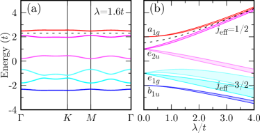
Figure 1: (Color online) (a) Noninteracting band dispersion with the hopping $t\,(>0)$ mediated by edge-sharing ligands for the SOC $\lambda=1.6t$. Each band is doubly degenerate (Kramer’s doublet). (b) Energy splitting of the noninteracting bands as a function of $\lambda$. Shade region represents the band width of each band. $a_{1g}$, $e_{2u}$, $e_{1g}$, and $b_{1u}$ refer to the symmetries of the quasimolecular bands when $\lambda=0$. Dotted lines in (a) and (b) denote the Fermi energy for $t_{2g}^{5}$ systems.

Correlation effect — Let us now explore the effect of electron correlations by considering a three-band Hubbard model on a periodic six-site cluster for electron density $n=5$ Supp with Lanczos exact diagonalization method Morgan93 ; Dagotto94 , which allows us to treat the electron kinetics inducing the QMO formation and the electron correlations on an equal footing, thus clearly going beyond the previous study BHKim2014 . We first examine the ground state as functions of the intra-orbital Coulomb repulsion $U$, Hund’s coupling $J_{\rm H}$, and $\lambda$, and check the stability of the QMO state. For this purpose, we calculate the hole density $\bar{n}_{a_{1g}}$ of the $a_{1g}$ quasimolecular band at the $\Gamma$ point, which is exactly one for the pure QMO state Supp . Figure 2(a) shows the result of $\bar{n}_{a_{1g}}$ for $J_{\rm H}=0$ with varying $U$ and $\lambda$. It clearly demonstrates that $\lambda$ and $U$ are both destructive perturbations to the QMOs. As already pointed out in Ref. Foyevtsova2013 , the strong SOC mixes the three $t_{2g}$ orbitals at each site, which gives rise to a finite overlap between the QMOs in neighboring hexagons, thus unfavorable to the QMO formation. More interestingly, we find here in Fig. 2(a) that the Coulomb repulsion is also adequate to destroy the QMO state. This is understood because the Coulomb interactions promote the scattering among electrons bounded in adjacent hexagons.

The ground state is described by a direct product of local states with not only $d^{5}$ electron configuration but also other configurations such as $d^{4}$ and $d^{6}$. Therefore, the ground state is sensitive to the local multiplet structures of these electron configurations. According to the multiplet theory, the Hund’s coupling $J_{\rm H}$ always brings about additional splitting of the $d^{4}$ multiplet hierarchy Supp . It is thus easily conjectured that $J_{\rm H}$ also plays a role in the QMO formation. Figure 2(b) well represents the effect of $J_{\rm H}$ on the QMO state. In finite $J_{\rm H}$, the region with the strong QMO character shrinks with somewhat smaller $\bar{n}_{a_{1g}}$ and the crossover boundary becomes sharper.

Figure 2: (Color online) The hole density $\bar{n}_{a_{1g}}$ of the $a_{1g}$ quasimolecular band at the $\Gamma$ point as functions of $U$ and $\lambda$ for (a) $J_{\rm H}=0$ and (b) $J_{\rm H}=1.6t$. Note that $\bar{n}_{a_{1g}}=1$ for the pure QMO state. The loci of Ru³⁺- and Ir⁴⁺-based $4d$ and $5d$ transition-metal compounds are also indicated.

In the whole parameter region of Fig. 2, the ground state is insulating. However, the insulating nature is expected to vary from a band insulator to a Mott insulator across the boundary where the QMO character is abruptly lost. To verify this conjecture, we calculate the excitation spectrum $\Lambda_{1/2}(\omega)$ of a doublon-holon pair formed in the $j_{\rm eff}=1/2$ orbitals at neighboring sites Supp , excitations schematically shown in ‘B’ of Fig. 3(d), which directly reflects the charge gap structure. As shown in Figs. 3(a)–(c), the $U$ dependence of $\Lambda_{1/2}(\omega)$ is qualitatively different across the crossover boundary. Below the boundary where the QMO character is strong, the low energy excitations shift downward in spite of increasing $U$, implying that an insulating gap evidently decreases with increasing the electron repulsion. In contrast, above the boundary where the QMO character is lost, the clear increase of the lowest peak position is manifested with increasing $U$, indicating the increase of the gap as in a Mott insulator. The similar feature is also found when $\lambda$ is increased with fixed $U$ and $J_{\rm H}$ Supp . These results support the conjecture that the insulating nature changes across the crossover boundary. The conjecture is further supported by other excitation spectra shown below.

Figure 3: (Color online) (a)–(c): Excitation spectrum $\Lambda_{1/2}(\omega)$ of a doublon-holon pair formed in the neighboring $j_{\rm eff}=1/2$ orbitals for (a) $\lambda=0.6t$, (b) $0.8t$, and (c) $1.6t$ with different $U-3J_{\rm H}$ values. $U-3J_{\rm H}$ varies from (a) $1.2t$ to $5.2t$, (b) $0$ to $4t$, and (c) $-1.6t$ to $2.4t$ with the same increment of $0.4t$. Solid triangles indicate peak positions of the exciton-like excitations in the RIXS spectrum for $U-3J_{\rm H}=5.2t$ (a), $4t$ (b), and $2t$ (c). We set $J_{\rm H}=1.6t$ and different line colors correspond to the values of $\bar{n}_{a_{1g}}$ shown in Fig. 2(b). (d) Schematic energy diagrams of three relevant electron-hole excitations. Blue solid and red dotted arrows refer to electron and hole, respectively, and up and down arrows denote Kramer’s doublet with positive (up arrow) and negative (down arrow) eigenvalues of $j^{z}_{\rm eff}$. “1” and “2” indicate two neighboring TM sites.

OC and RIXS spectra — The Kubo formula and the continued fraction method are exploited to investigate the OC and $L_{3}$-edge RIXS spectra Supp . Figure 4 summarizes the results for $\lambda=0.6t$, 0.8$t$, and 1.6$t$ with $J_{\rm H}$=$1.6t$. Note that the QMO character suddenly diminishes at $U-3J_{\rm H}\sim 3t$ for $\lambda=0.6t$, $2t$ for $0.8t$, and $0$ for $1.6t$, as shown in Fig. 2(b). The abrupt change of the electronic characteristics is reflected in these excitation spectra.

When the QMO character is strong with large $\bar{n}_{a_{1g}}$, the OC exhibits a two-peak structure for $\lambda=0.6t$ and $0.8t$, and a three-peak structure for $\lambda=1.6t$. The lower (higher) peak in the OC is attributed to the transition between the $a_{1g}$ and $e_{2u}$ ($e_{1g}$) quasimolecular bands whose energies are around $t$ ($3t$) (see Fig. 1). The large splitting of the $e_{2u}$ bands for the strong SOC can give an additional splitting to the lower peak in the OC. The RIXS spectrum also shows the similar peak structures near the similar excitation energies. Consequently, the excitations can be interpreted on the basis of the single-particle picture. Therefore, a strong band insulating character is predominant in this region.

In the region where the QMO character is degraded, the OC shows a one-peak structure and the peak position monotonically increases with $U$, while the RIXS spectra exhibits the dominant peak around $3\lambda/2$ in addition to an almost zero energy peak due to the magnetic excitation. These features can be well understood as on-site or inter-site electron-hole excitations in the local relativistic $j_{\rm eff}$ orbitals. As shown in ‘B’ and ‘C’ of Fig. 3(d), two types of inter-site electron-hole excitations can play a role in the OC. However, the edge-shared geometry suppresses the contribution of type ‘B’ electron-hole excitation simply because the hopping between the neighboring $j_{\rm eff}=1/2$ orbitals is zero hopJ . Hence, only type ‘C’ electron-hole excitation gives the dominant contribution to form the one-peak like structure at excitation energy $\omega\approx U-3J_{\rm H}+\frac{3\lambda}{2}$. In the RIXS spectrum, an on-site electron-hole excitation indicated in ‘A’ of Fig. 3(d), i.e., a local $d$-$d$ transition between the $j_{\rm eff}=3/2$ and $1/2$ orbitals, can give a dominant intensity at $\omega\approx 3\lambda/2$. Thus, both OC and RIXS spectra in this region can be interpreted in terms of the relativistic Mott insulating picture.

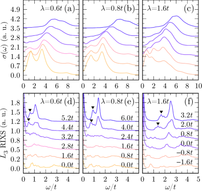
Figure 4: (Color online) (a)–(c) OC $\sigma(\omega)$ and (d)–(f) $L_{3}$-edge RIXS spectrum at wave number $\mathbf{q}=0$ for $\lambda=0.6t$ [(a) and (d)], $0.8t$ [(b) and (e)], and $1.6t$ [(c) and (f)] with various $U-3J_{\rm H}$ values indicated in the figures. We set $J_{\rm H}=1.6t$ and different line colors correspond to the values of $\bar{n}_{a_{1g}}$ shown in Fig. 2(b). The exciton-like excitations in the RIXS spectrum are indicated by solid triangles in (d)–(f).

In the relativistic Mott insulating limit, the RIXS spectrum shows an additional peak below the local $d$-$d$ excitation ($\approx 3\lambda/2$) and above the almost zero energy magnetic peak, which is marked by triangles in Figs. 4(d)–(f). Indeed, this peak has been observed in Na₂IrO₃ and the origin is attributed to the exciton formation induced by the inter-site electron correlations Gretarsson2013 . However, the consecutive theoretical study based on the strong coupling model calculations has shown that this exciton-like peak appears even without considering the inter-site electron correlations when the inter-site migration of electrons from the $j_{\rm eff}=1/2$ to $3/2$ orbitals [‘B’ of Fig. 3(d)] follows the local $d$-$d$ transition [‘A’ of Fig. 3(d)], resulting in the inter-site electron-hole excitation between the $j_{\rm eff}=1/2$ orbitals BHKim2014 . As shown in Figs. 3(a)–(c), the excitation spectrum $\Lambda_{1/2}(\omega)$ of a doublon-holon pair in the $j_{\rm eff}=1/2$ orbitals also yield the obvious spectral weight in the vicinity of the exciton-like RIXS excitation energy, implying that these excitations are due to the same origin. In addition, the monotonic increase of the exciton-like peak position in the RIXS spectrum with $U$ is also consistent with $\Lambda_{1/2}(\omega)$. We also find that the intensity of the exciton-like RIXS peak depends strongly on momentum Supp , which is in good agreement with the experiments Gretarsson2013 . Thus, it is reasonable to infer that the origin of the exciton-like peak near the edge of local $d$-$d$ excitation in the RIXS is due to the combined excitations of two different types (‘A’ and ‘B’).

Ir⁴⁺- and Ru³⁺-based systems — A typical SOC is known to be $0.4$–$0.5$ eV for $5d$ systems and $0.1$–$0.2$ eV for $4d$ systems Dai2008 ; Clancy2012 . Recent theoretical studies have estimated that $t\approx 0.27$ eV for the most studied Ir⁴⁺ system Na₂IrO₃ Mazin2012 ; Foyevtsova2013 ; Yamaji2014 , and $t\approx 0.11$ eV HSKim2015 and $0.16$ eV Winter2016 for $\alpha$-RuCl₃ (Ru³⁺), both of which are much smaller than that for Ir⁴⁺ systems. $U$ and $J_{\rm H}$, however, are not easy to be determined because the full screening effect of electron correlations is hardly treated. One useful expedient is to extract them from the OC measurement.

Since the dominant optical peak appears near $U-3J_{\rm H}+\frac{3\lambda}{2}$, we can estimate $U-3J_{\rm H}\sim 0.8$–$1.0$ eV for Na₂IrO₃ based on the existing OC data, which exhibits a one-peak structure around 1.6 eV Comin2012 ; Sohn2013 . Assuming $U-3J_{\rm H}=3.2t$ ($\approx 0.86$ eV), our results for the OC and RIXS spectra in Figs. 4(c) and (f) are both indeed in good quantitative agreement with the experiments Comin2012 ; Sohn2013 ; Gretarsson2013 , except for a double-peak structure around 0.7 eV ($\approx 2.6t$) observed in the RIXS experiment, instead of a single peak found in Fig. 4(f). Here, our calculations assume the cubic crystal field. However, the crystal structure of Na₂IrO₃ is known to display the additional trigonal distortion note , thus significantly departing from the ideal IrO₆ octahedra Choi2012 . This additional distortion can mix the relativistic $j_{\rm eff}=1/2$ and $3/2$ orbitals, and lead to the splitting of the dominant RIXS peak of the local $d$-$d$ transition into multiple subpeaks Liu2012 ; Plotnikova2016 . Indeed, we find that the single peak found in Fig. 4(f) is split into two (or multiple) subpeaks in the presence of the trigonal distortion Supp (see also Refs. Gretarsson2013 ; BHKim2014 ). Therefore, we can conclude that the electronic state of Na₂IrO₃ is far from the QMO limit and is located in the relativistic Mott insulating region, as indicated in Fig. 2.

The recent optical absorption experiments for $\alpha$-RuCl₃ have found a dominant peak around 1.2 eV as well as a small additional peak near 0.3 eV Plumb2014 ; Sandilands2016 . The photoemission spectroscopy measurement has also observed a large gap about 1.2 eV Koitzsch2016 . Thus, $U-3J_{\rm H}$ for $\alpha$-RuCl₃ is estimated to be about 0.9–1.1 eV. Adopting $t=0.16$ eV, our result for $U-3J_{\rm H}=6t$ ($\approx 0.96$ eV) and $\lambda=0.8t$ ($\approx 0.13$ eV) in Fig. 4(b) also exhibits the dominant peak near 1.1 eV ($\approx 6.9t$). Although no experimental RIXS spectrum has been reported yet, the recent neutron scattering measurement on $\alpha$-RuCl₃ observed an inelastic peak near 195 meV and estimated that $\lambda\approx 130$ meV Banerjee2016 . This observation is consistent with a dominant RIXS peak around $1.4t$ ($\approx 0.22$ eV) for $U-3J_{\rm H}=6t$ in Fig. 4(e). Therefore, we expect that $\alpha$-RuCl₃ is located also in the QMO poor region, as indicated in Fig. 2.

It should be noted, however, that the OC for $U-3J_{\rm H}=6t$ in Fig. 4(b) fails to yield the low-energy peak near 0.3 eV observed experimentally in $\alpha$-RuCl₃. This can be explained by considering an additional direct $d$-$d$ hopping $t^{\prime}$ between neighboring sites, estimated as large as $-0.23$ eV in Ref. HSKim2015 and $-0.15$ eV in Ref. Winter2016 . As discussed in Supplemental Material Supp , the low-energy peak attributed to the local $d$-$d$ transition [‘A’ in Fig. 3(d)] can emerge because the forbidden optical transition among the $j_{\rm eff}=1/2$ bands without the direct hopping $t^{\prime}$ can now be accessed in the presence of $t^{\prime}$ OCRuCl3 . The experimental fact that the intensity of the low-energy peak near 0.3 eV is much weaker than that of the dominant peak around 1.2 eV suggests that the strength of $t^{\prime}$ is not as large as the theoretical estimation Supp .

Conclusion — Based on the numerically exact diagonalization analyses of the three-band Hubbard model, we have shown that the ground state of the $t_{2g}^{5}$ system with the honeycomb lattice structure can be transferred from the quasimolecular band insulator to the relativistic Mott insulator with increasing $\lambda$ as well as $U$ when the QMOs are disturbed and eventually replaced by the local relativistic $j_{\rm eff}$ orbitals. We have demonstrated that the different electronic nature of these insulators is manifested in the electronic excitations observed in OC and RIXS. Comparing our results with experiments, we predict that not only Na₂IrO₃ with strong SOC but also $\alpha$-RuCl₃ with moderate SOC is the relativistic Mott insulator. This deserves further experimental confirmation, especially for $\alpha$-RuCl₃ where we expect the exciton-like excitation near the edge of the local $d$-$d$ excitation in the RIXS spectrum.

Acknowledgements — The numerical computations have been performed with the RIKEN supercomputer system (HOKUSAI GreatWave). This work has been supported by Grant-in-Aid for Scientific Research from MEXT Japan under the Grant No. 25287096 and also by RIKEN iTHES Project and Molecular Systems.

I Hamiltonian

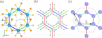
Figure S1: (a) Schematic crystal structure of the honeycomb lattice TM systems, (b) its accessible hopping between neighboring TMs mediated via two edge-sharing ligands, and (c) a periodic six-site cluster (containing $M_{1},M_{2},\dots$, and $M_{6}$ sites surrounded by dashed lines) employed for the calculations. TMs ($M$) are denoted by blue spheres and ligands ($L$) above (below) the hexagon plane formed by TMs are indicated by orange (yellow) spheres in (a). $XY$, $YZ$, and $ZX$ in (b) refer to three $t_{2g}$ orbitals ($d_{XY}$, $d_{YZ}$, and $d_{ZX}$, respectively) in the local coordinates $X$, $Y$, and $Z$ defined in (a). As indicated by double head arrows in (b), the electron motion is bounded in each hexagon due to the bond-dependent hoppings when the SOC and Coulomb interaction are both absent. Red, green, and blue bonds in (a)–(c) represent the $XY$-, $YZ$-, and $ZX$-directions, respectively (also see TABLE S1). The unit lattice vectors $\vec{a}_{1}=\sqrt{3}a\hat{x}$ and $\vec{a}_{2}=-\frac{\sqrt{3}a}{2}\hat{x}+\frac{3a}{2}\hat{y}$ of the honeycomb lattice are also indicated in (c), where the global coordinates $x$, $y$, and $z$ are given in (a), and $\hat{x}$, $\hat{y}$, and $\hat{z}$ are unit vectors along the $x$-, $y$-, and $z$-directions, respectively.

As shown in Fig. S1(a), transition metal (TM) ions in the honeycomb lattice systems studied in the main text such as Na₂IrO₃ and $\alpha$-RuCl₃ are connected via two edge-sharing ligands. To describe the electronic structure of these systems, we adopt the three-band Hubbard Hamiltonian in the honeycomb lattice defined as

$$H= \sum_{i,\delta,\mu,\nu,\sigma}t_{\mu\nu}^{\delta}c_{i_{\delta}\mu\sigma}^{\dagger}c_{i\nu\sigma}+\lambda\sum_{i,\mu,\nu,\sigma,\sigma^{\prime}}(\mathbf{l}\cdot\mathbf{s})_{\mu\sigma,\nu\sigma^{\prime}}c_{i\mu\sigma}^{\dagger}c_{i\nu\sigma^{\prime}}$$

$$+\frac{1}{2}\sum_{i,\sigma,\sigma^{\prime},\mu,\nu}U_{\mu\nu}c_{i\mu\sigma}^{\dagger}c_{i\nu\sigma^{\prime}}^{\dagger}c_{i\nu\sigma^{\prime}}c_{i\mu\sigma}+\frac{1}{2}\sum_{\begin{subarray}{c}i,\sigma,\sigma^{\prime},\mu,\nu\\ (\mu\neq\nu)\end{subarray}}J_{\mu\nu}c_{i\mu\sigma}^{\dagger}c_{i\nu\sigma^{\prime}}^{\dagger}c_{i\mu\sigma^{\prime}}c_{i\nu\sigma}+\frac{1}{2}\sum_{\begin{subarray}{c}i,\sigma,\mu,\nu\\ (\mu\neq\nu)\end{subarray}}J_{\mu\nu}^{\prime}c_{i\mu\sigma}^{\dagger}c_{i\mu\bar{\sigma}}^{\dagger}c_{i\nu\bar{\sigma}}c_{i\nu\sigma},$$ (S1)

where $c_{i\nu\sigma}^{\dagger}$ is the creation operator of an electron with orbital $\nu\,(=XY,YZ,ZX)$ and spin $\sigma\,(=\uparrow,\downarrow)$ at site $i$ in the honeycomb lattice, and three $t_{2g}$ orbitals $XY$, $YZ$, and $ZX$ correspond respectively to $d_{XY}$, $d_{YZ}$, and $d_{ZX}$ orbitals defined in the local octahedron coordinates ($X$, $Y$, and $Z$), as indicated in Fig. S1(a). $\delta$ in the first term denotes the three nearest neighbor (NN) directions in the honeycomb lattice (i.e., $XY$-, $YZ$-, and $ZX$-directions, as indicated in Fig. S1) and $i_{\delta}$ is the $\delta$-directional NN site from site $i$. $\bar{\sigma}$ stands for the opposite spin of $\sigma$. The NN hopping matrix $t_{\mu\nu}^{\delta}$ is given in TABLE S1 and the nonzero NN hoppings are schematically summarized in Fig. S1(b). The second term in the right hand side of Eq. (S1) describes the spin-orbit coupling (SOC) with the coupling constant $\lambda$, where $\mathbf{l}$ and $\mathbf{s}$ denote the orbital and spin angular momentum operators, respectively. The last three terms in the right hand side of Eq. (S1) represent the two-body Coulomb interactions, where we assume the Kanamori-type Coulomb interaction, i.e., $U_{\mu\mu}=U$, $U_{\mu\neq\nu}=U-2J_{\rm H}$, and $J_{\mu\nu}=J_{\mu\nu}^{\prime}=J_{\rm H}$ S (1).

Table S1: Hopping matrix $t_{\mu\nu}^{\delta}$ along three different directions. The $XY$-, $YZ$-, and $ZX$-directions refer to the bond directions along which the NN TMs are connected via the two edge-sharing ligands located in the $XY$-, $YZ$-, and $ZX$-planes, respectively [see Fig. S1(a)]. $|ZX\rangle$, $|XY\rangle$, and $|YZ\rangle$ represent the three $t_{2g}$ orbitals, i.e., $d_{ZX}$, $d_{XY}$, and $d_{YZ}$, respectively, defined in the local coordinates $X$, $Y$, and $Z$, as indicated in Fig. S1(a).

	$XY$-direction	$YZ$-direction	$ZX$-direction
	$\begin{matrix}&|ZX\rangle&|XY\rangle&|YZ\rangle\\ \langle ZX|&0&0&t\\ \langle XY|&0&0&0\\ \langle YZ|&t&0&0\end{matrix}$	$\begin{matrix}&|ZX\rangle&|XY\rangle&|YZ\rangle\\ \langle ZX|&0&t&0\\ \langle XY|&t&0&0\\ \langle YZ|&0&0&0\end{matrix}$	$\begin{matrix}&|ZX\rangle&|XY\rangle&|YZ\rangle\\ \langle ZX|&0&0&0\\ \langle XY|&0&0&t\\ \langle YZ|&0&t&0\end{matrix}$

Let us define the local orbitals $\tilde{y}$, $\tilde{z}$, and $\tilde{x}$ as

$$|\tilde{y}\rangle = \frac{1}{\sqrt{2}}\left(|ZX\rangle-|YZ\rangle\right),$$ (S2)

$$|\tilde{z}\rangle = \frac{1}{\sqrt{3}}\left(|ZX\rangle+|XY\rangle+|YZ\rangle\right),$$ (S3)

$$|\tilde{x}\rangle = \frac{1}{\sqrt{6}}\left(|ZX\rangle-2|XY\rangle+|YZ\rangle\right),$$ (S4)

which correspond to $\sqrt{\frac{2}{3}}d_{xy}\!-\!\sqrt{\frac{1}{3}}d_{yz}$, $d_{z^{2}}$, and $-\sqrt{\frac{2}{3}}d_{x^{2}-y^{2}}\!-\!\sqrt{\frac{1}{3}}d_{zx}$, respectively, in the global coordinates $x$, $y$, and $z$ of the honeycomb lattice [see Fig. S1(a)].

Notice that the unitary transformation given above from $ZX$, $XY$, and $YZ$ orbitals to $\tilde{y}$, $\tilde{z}$, and $\tilde{x}$ orbitals is exactly the same as that for $p$ orbitals from $p_{Y}$, $p_{Z}$, and $p_{X}$ orbitals in the local coordinates to $p_{y}$, $p_{z}$, and $p_{x}$ orbitals in the global coordinates. With these orbitals as the basis set, the SOC is nonzero only for $\langle\tilde{x}\sigma|\mathbf{l}\cdot\mathbf{s}|\tilde{y}\sigma\rangle=\frac{i}{2}s_{\sigma}$, $\langle\tilde{y}\sigma|\mathbf{l}\cdot\mathbf{s}|\tilde{z}\bar{\sigma}\rangle=\frac{i}{2}$, and $\langle\tilde{z}\sigma|\mathbf{l}\cdot\mathbf{s}|\tilde{x}\bar{\sigma}\rangle=\frac{1}{2}s_{\sigma}$, where $s_{\sigma}=1\,(-1)$ for $\sigma=\uparrow\,(\downarrow)$ and the imaginary unit $i$ should not be confused with the site index $i$ in Eq. (S1). The local SOC term can be readily diagonalized in terms of the relativistic orbitals with the effective total angular momentum $j_{\rm eff}=1/2$, i.e.,

$$|j_{\rm eff}=1/2,j_{\rm eff}^{z}=+1/2\rangle =-\frac{1}{\sqrt{3}}\left(|\tilde{z}+\rangle+|\tilde{x}-\rangle+i|\tilde{y}-\rangle\right),$$ (S5)

$$|j_{\rm eff}=1/2,j_{\rm eff}^{z}=-1/2\rangle =+\frac{1}{\sqrt{3}}\left(|\tilde{z}-\rangle-|\tilde{x}+\rangle+i|\tilde{y}+\rangle\right),$$ (S6)

and those with $j_{\rm eff}=3/2$, i.e.,

$$|j_{\rm eff}=3/2,j_{\rm eff}^{z}=+3/2\rangle =-\frac{1}{\sqrt{2}}\left(|\tilde{x}+\rangle+i|\tilde{y}+\rangle\right),$$ (S7)

$$|j_{\rm eff}=3/2,j_{\rm eff}^{z}=+1/2\rangle =+\frac{1}{\sqrt{6}}\left(2|\tilde{z}+\rangle-|\tilde{x}-\rangle-i|\tilde{y}-\rangle\right),$$ (S8)

$$|j_{\rm eff}=3/2,j_{\rm eff}^{z}=-1/2\rangle =+\frac{1}{\sqrt{6}}\left(2|\tilde{z}-\rangle+|\tilde{x}+\rangle-i|\tilde{y}+\rangle\right),$$ (S9)

$$|j_{\rm eff}=3/2,j_{\rm eff}^{z}=-3/2\rangle =+\frac{1}{\sqrt{2}}\left(|\tilde{x}-\rangle-i|\tilde{y}-\rangle\right),$$ (S10)

whose energies are $\lambda$ for $j_{\rm eff}=1/2$ and $-\lambda/2$ for $j_{\rm eff}=3/2$.

II Quasimolecular bands

Let us define the unit lattice vectors $\vec{a}_{1}=\sqrt{3}a\hat{x}$ and $\vec{a}_{2}=-\frac{\sqrt{3}a}{2}\hat{x}+\frac{3a}{2}\hat{y}$ of the honeycomb lattice [see Fig. S1(c)], where $a$ is the lattice constant between NN sites. Note that the unit cell contains two basis sites, “1” and “2”, located at $\mathbf{0}$ and $a\hat{y}$, respectively. The unit reciprocal lattice vectors are thus given as $\vec{b}_{1}=\frac{4\pi}{2\sqrt{3}a}\big{(}\hat{x}+\frac{1}{\sqrt{3}}\hat{y}\big{)}$ and $\vec{b}_{2}=\frac{4\pi}{3a}\hat{y}$.

In the non-interacting limit with $\lambda=0$, the Hamiltonian $H$ can be expressed simply by the following tight-binding Hamiltonian

$$H_{t}=\sum_{\mathbf{k}}\sum_{\alpha,\beta}\sum_{i,j}\sum_{\sigma}H_{\alpha_{i}\beta_{j}}(\mathbf{k})c_{\alpha_{i}\sigma}^{\dagger}(\mathbf{k})c_{\beta_{j}\sigma}(\mathbf{k}),$$ (S11)

where $c_{\alpha_{i}\sigma}^{\dagger}(\mathbf{k})$ is the Fourier transformation of the creation operator of an electron with orbital $\alpha$ and spin $\sigma$ at the $i$-th basis site ($i=1,2$). The Hamiltonian matrix $H(\mathbf{k})$ is given as

$$H(\mathbf{k})=\begin{pmatrix}0&0&0&0&te^{i(k_{1}+k_{2})}&t\\ 0&0&0&te^{i(k_{1}+k_{2})}&0&te^{ik_{2}}\\ 0&0&0&t&te^{ik_{2}}&0\\ 0&te^{-i(k_{1}+k_{2})}&t&0&0&0\\ te^{-i(k_{1}+k_{2})}&0&te^{-ik_{2}}&0&0&0\\ t&te^{-ik_{2}}&0&0&0&0\end{pmatrix}$$ (S12)

in the basis of $(ZX_{1},XY_{1},YZ_{1},ZX_{2},XY_{2},YZ_{2})$ for wave number $\mathbf{k}=\frac{k_{1}}{2\pi}\vec{b}_{1}+\frac{k_{2}}{2\pi}\vec{b}_{2}$ with $k_{1}$ and $k_{2}$ being real numbers.

Introducing the $(3\times 3)$ matrix

$$A(\mathbf{k})=\begin{pmatrix}0&te^{i(k_{1}+k_{2})}&t\\ te^{i(k_{1}+k_{2})}&0&te^{ik_{2}}\\ t&te^{ik_{2}}&0\end{pmatrix},$$ (S13)

the Hamiltonian matrix $H(\mathbf{k})$ is expressed as

$$H(\mathbf{k})=\begin{pmatrix}0&A(\mathbf{k})\\ A(\mathbf{k})^{\dagger}&0\end{pmatrix}.$$ (S14)

Let the eigenvalue and the eigenstate of $H(\mathbf{k})$ be $E$ and $\mathbf{X}_{E}=\begin{pmatrix}X&Y\end{pmatrix}^{\textrm{T}}$, respectively. Because

$$\begin{pmatrix}0&A(\mathbf{k})\\ A(\mathbf{k})^{\dagger}&0\end{pmatrix}\begin{pmatrix}X\\ Y\end{pmatrix}=E\begin{pmatrix}X\\ Y\end{pmatrix},$$ (S15)

$A(\mathbf{k})Y=EX$ and $A(\mathbf{k})^{\dagger}X=EY$. We can thus rewrite the eigenvalue problem as

$$A(\mathbf{k})A(\mathbf{k})^{\dagger}X=t^{2}\begin{pmatrix}2&e^{-ik_{2}}&e^{ik_{1}}\\ e^{ik_{2}}&2&e^{i(k_{1}+k_{2})}\\ e^{-ik_{1}}&e^{-i(k_{1}+k_{2})}&2\end{pmatrix}X=E^{2}X.$$ (S16)

By solving the above equation, we can obtain the following eigenstates

$$X_{1}^{\textrm{T}}=\begin{pmatrix}1,&e^{ik_{2}},&e^{-ik_{1}}\end{pmatrix},$$ (S17)

$$X_{2}^{\textrm{T}}=\begin{pmatrix}0,&e^{ik_{2}},&-e^{-ik_{1}}\end{pmatrix},$$ (S18)

$$X_{3}^{\textrm{T}}=\begin{pmatrix}-2,&e^{ik_{2}},&e^{-ik_{1}}\end{pmatrix},$$ (S19)

whose eigenvalues $E^{2}$ are $4t^{2}$, $t^{2}$, and $t^{2}$, respectively. Since $Y=\frac{1}{E}A(\mathbf{k})^{\dagger}X$, we finally obtain the six eigenstates of $H(\mathbf{k})$ as

$$\mathbf{X}_{a_{1g}}(\mathbf{k})=\frac{1}{\sqrt{6}}\begin{pmatrix}1,&e^{ik_{2}},&e^{-ik_{1}},&e^{-ik_{1}},&e^{-i(k_{1}+k_{2})},&1\end{pmatrix}^{\textrm{T}},$$ (S20)

$$\mathbf{X}_{e_{2u,1}}(\mathbf{k})=\frac{1}{2}\begin{pmatrix}0,&e^{ik_{2}},&-e^{-ik_{1}},&0,&-e^{-i(k_{1}+k_{2})},&1\end{pmatrix}^{\textrm{T}},$$ (S21)

$$\mathbf{X}_{e_{2u,2}}(\mathbf{k})=\frac{1}{2\sqrt{3}}\begin{pmatrix}-2,&e^{ik_{2}},&e^{-ik_{1}},&2e^{-ik_{1}},&-e^{-i(k_{1}+k_{2})},&-1\end{pmatrix}^{\textrm{T}},$$ (S22)

$$\mathbf{X}_{e_{1g,1}}(\mathbf{k})=\frac{1}{2}\begin{pmatrix}0,&e^{ik_{2}},&-e^{-ik_{1}},&0,&e^{-i(k_{1}+k_{2})},&-1\end{pmatrix}^{\textrm{T}},$$ (S23)

$$\mathbf{X}_{e_{1g,2}}(\mathbf{k})=\frac{1}{2\sqrt{3}}\begin{pmatrix}-2,&e^{ik_{2}},&e^{-ik_{1}},&-2e^{-ik_{1}},&e^{-i(k_{1}+k_{2})},&1\end{pmatrix}^{\textrm{T}},$$ (S24)

$$\mathbf{X}_{b_{1u}}(\mathbf{k})=\frac{1}{\sqrt{6}}\begin{pmatrix}1,&e^{ik_{2}},&e^{-ik_{1}},&-e^{-ik_{1}},&-e^{-i(k_{1}+k_{2})},&-1\end{pmatrix}^{\textrm{T}},$$ (S25)

with the eigenvalues being $2t$, $t$, $t$, $-t$, $-t$, and $-2t$, respectively. Because all eigenvalues are wave number independent, we can call these energy bands as quasimolecular bands formed by quasimolecular orbitals (QMOs) with their symmetries, $a_{1g}$, $e_{2u}$, $e_{1g}$, and $b_{1u}$, indicated in the above eigenstates.

III cluster calculations

To explore the correlation effect, we consider a periodic six-site cluster shown in Fig S1(c), which contains six holes for the $t_{2g}^{5}$ systems discussed in the main text. We take into account all states to represent the whole Hilbert space and thus the size of the Hilbert space is ${}_{36}C_{6}=1947792$. To solve Eq. (S1) and find the ground state, we employ the exact diagonalization method based on Lanczos algorithm with the Jacobi preconditioner S (2). We obtain the ground state and the corresponding eigenenergy with the energy accuracy of $4\times 10^{-10}t$.

III.1 Hole density of $a_{1g}$ band

Since only the $a_{1g}$ band is fully empty in the non-relativistic and non-interacting limits for the $t_{2g}^{5}$ systems, the hole density in the $a_{1g}$ quasimolecular band is a good quantity to quantify how far the ground state is from the pure QMO state. The hole density operator $\bar{\rho}_{a_{1g}}(\mathbf{k})$ per site at the wave number $\mathbf{k}$ is defined as

$$\bar{\rho}_{a_{1g}}(\mathbf{k})=\frac{1}{2}\sum_{\sigma}c_{a_{1g}\sigma}(\mathbf{k})c^{\dagger}_{a_{1g}\sigma}(\mathbf{k}),$$ (S26)

where the creation operator $c^{\dagger}_{a_{1g}\sigma}(\mathbf{k})$ is the eigenstate of $H({\mathbf{k}})$ and is given as $c^{\dagger}_{a_{1g}\sigma}(\mathbf{k})=\sum_{j,\nu}[\mathbf{X}_{a_{1g}}(\mathbf{k})]_{\nu_{j}}c^{\dagger}_{\nu_{j}\sigma}(\mathbf{k}).$ Here $[\mathbf{X}_{a_{1g}}(\mathbf{k})]_{\nu_{j}}$ ($j=1,2$ and $\nu=ZX,XY,YZ$) is the $\nu_{j}$-th element of the eigenstate of $H(\mathbf{k})$ with $a_{1g}$ symmetry given in Eq. (S20). For the six-site cluster with periodic boundary conditions, there exist three independent wave numbers, i.e., $(k_{1},k_{2})=(0,0)$ ($\Gamma$ point), $(\frac{\pi}{3},\frac{\pi}{3})$ ($K$ point), and $(\frac{2\pi}{3},\frac{2\pi}{3})$ ($K^{\prime}$ point), and $c^{\dagger}_{a_{1g}\sigma}(\mathbf{k})$ for these wave numbers are expressed as

$$c^{\dagger}_{a_{1g}\sigma}(\mathbf{k}) =\frac{1}{\sqrt{3}}\Big{(}\sum_{\nu}[\mathbf{X}_{a_{1g}}(\mathbf{k})]_{\nu_{1}}c^{\dagger}_{1\nu\sigma}+\sum_{\nu}[\mathbf{X}_{a_{1g}}(\mathbf{k})]_{\nu_{2}}c^{\dagger}_{2\nu\sigma}+\sum_{\nu}[\mathbf{X}_{a_{1g}}(\mathbf{k})]_{\nu_{1}}e^{-i(k_{1}+k_{2})}c^{\dagger}_{3\nu\sigma}$$

$$+\sum_{\nu}[\mathbf{X}_{a_{1g}}(\mathbf{k})]_{\nu_{2}}e^{-ik_{1}}c^{\dagger}_{4\nu\sigma}+\sum_{\nu}[\mathbf{X}_{a_{1g}}(\mathbf{k})]_{\nu_{1}}e^{-ik_{1}}c^{\dagger}_{5\nu\sigma}+\sum_{\nu}[\mathbf{X}_{a_{1g}}(\mathbf{k})]_{\nu_{2}}e^{ik_{2}}c^{\dagger}_{6\nu\sigma}\Big{)},$$ (S27)

where $c^{\dagger}_{j\nu\sigma}$ is the creation operator of an electron with orbital $\nu=(YZ,ZX,XY)$ and spin $\sigma=(\uparrow,\downarrow)$ at site $M_{j}$ in the six-site cluster shown in Fig. S1(c). In the main text, we calculate the hole density at the $\Gamma$ point, i.e.,

$$\bar{n}_{a_{1g}}=\langle\Psi_{0}|\bar{\rho}_{a_{1g}}(\mathbf{k}=0)|\Psi_{0}\rangle,$$ (S28)

where $|\Psi_{0}\rangle$ is the ground state of the six-site cluster. This quantity $\bar{n}_{a_{1g}}$ is exactly one for the pure QMO state.

III.2 Doublon-holon excitations in $j_{\rm eff}=1/2$ orbitals

To explore the distribution of a doublon-holon pair in the $j_{\rm eff}=1/2$ orbitals at neighboring sites, we calculate the projected spectrum

$$\Lambda_{1/2}(\omega) =\sum_{n}\sum_{s_{3},s_{4},s_{5},s_{6}}\left|\langle D_{s_{3},s_{4},s_{5},s_{6}}|\Psi_{n}\rangle\right|^{2}\delta(\omega-E_{n}+E_{0})$$

$$=-\frac{1}{\pi}\textrm{Im}\sum_{s_{3},s_{4},s_{5},s_{6}}\langle D_{s_{3},s_{4},s_{5},s_{6}}|\frac{1}{\omega-H+E_{0}+i\delta}|D_{s_{3},s_{4},s_{5},s_{6}}\rangle,$$ (S29)

where $|\Psi_{n}\rangle$ and $E_{n}$ are the $n$-th eigenstate and eigenvalue of $H$, respectively, and the ground state corresponds to $n=0$. $|D_{s_{3},s_{4},s_{5},s_{6}}\rangle$ is a single doublon-holon pair excited state in the NN $j_{\rm eff}=1/2$ orbitals at sites $M_{1}$ and $M_{2}$ [see Fig. S1(c)], defined as

$$|D_{s_{3},s_{4},s_{5},s_{6}}\rangle=d_{1,+1/2}d_{1,-1/2}d_{3,s_{3}}d_{4,s_{4}}d_{5,s_{3}}d_{6,s_{6}}|\textrm{FO}\rangle,$$ (S30)

where $|\textrm{FO}\rangle$ is the fully occupied state with electrons and $d_{l,s_{l}}$ is the annihilation operator of $j_{\rm eff}=1/2$ electron with isospin $s_{l}\,(=\pm 1/2)$ [given in Eqs. (S5) and (S6)] at site $M_{l}$ in the six-site cluster shown in Fig. S1(c). To calcuate $\Lambda_{1/2}(\omega)$, we employ the continued faction method S (3). We perform 500 iterations of the continued faction with $\delta=0.12t$.

As shown in Figs. 3(a)–(c) of the main text, the $U$ dependence of the low-energy peak positions in $\Lambda_{1/2}(\omega)$ for given $\lambda$ is qualitatively different in the two insulators, i.e., the quasimolecular band insulator and the relativistic Mott insulator. As shown in Fig. S2, the similar change of behavior is found even when $\lambda$ is varied for fixed $U$ and $J_{\rm H}$. With increasing $\lambda$, the low-energy peak positions first shift downward in energy and then move upward once we cross the crossover region. The increase of the low-energy peak positions supports that the edge of $\Lambda_{1/2}(\omega)$ in the relativistic Mott limit is evidently coupled with the local $d$-$d$ excitation, whose excitation energy is proportional to $\lambda$. Therefore, the exciton-like peak as well as the spin-orbit exciton peak in the RIXS spectrum should also shift upward with increasing $\lambda$. The decrease of the low-energy peak positions in $\Lambda_{1/2}(\omega)$ in the QMO limit is due to the decrease of a band gap with increasing $\lambda$, as shown in Fig. 1(b) of the main text.

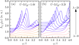
Figure S2: (Color online) Doublon-holon excitation spectrum $\Lambda_{1/2}(\omega)$ for $U-3J_{\rm H}=1.6t$ (a) and $3.2t$ (b) with varying $\lambda$ indicated in the figure. Here we set $J_{\rm H}=1.6t$ and different line colors correspond to the values of $\bar{n}_{a_{1g}}$ shown in Fig. 2(b) of the main text.

III.3 Optical conductivity

We adopt the Kubo formula to calculate the optical conductivity (OC),

$$\sigma(\omega) =\frac{\pi v}{\omega}\sum_{n(\neq 0)}|\langle\Psi_{n}|\hat{J}_{c}|\Psi_{0}\rangle|^{2}\delta(\omega-E_{n}\!+\!E_{0})$$

$$=-v\ \textrm{Im}\sum_{n(\neq 0)}\frac{|\langle\Psi_{n}|\hat{J}_{c}|\Psi_{0}\rangle|^{2}}{(E_{n}-E_{0})(\omega-E_{n}\!+\!E_{0}+i\delta)}$$

$$=-v\ \textrm{Im}\Big{[}\frac{1}{\omega+i\delta}\sum_{n(\neq 0)}\Big{(}\frac{|\langle\Psi_{n}|\hat{J}_{c}|\Psi_{0}\rangle|^{2}}{E_{n}-E_{0}}+\frac{|\langle\Psi_{n}|\hat{J}_{c}|\Psi_{0}\rangle|^{2}}{\omega-E_{n}\!+\!E_{0}+i\delta}\Big{)}\Big{]}$$

$$=-v\ \textrm{Im}\Big{[}\frac{1}{\omega+i\delta}\Big{(}\langle\Psi_{0}|\hat{J}_{c}\frac{1}{H-E_{0}}\hat{J}_{c}|\Psi_{0}\rangle+\langle\Psi_{0}|\hat{J}_{c}\frac{1}{\omega-H+E_{0}+i\delta}\hat{J}_{c}|\Psi_{0}\rangle\Big{)}\Big{]},$$ (S31)

where $v$ is the volume per site and $\hat{J}_{c}$ is the current operator along the $XY$-direction given as

$$\hat{J}_{c}=-\frac{ie}{A\hbar}\sum_{\mu,\nu,\sigma}\big{(}t^{XY}_{\mu\nu}c_{2\nu\sigma}^{\dagger}c_{1\mu\sigma}-t^{XY}_{\mu\nu}c_{1\mu\sigma}^{\dagger}c_{2\nu\sigma}\big{)},$$ (S32)

where $e\,(<0)$ is the electronic charge and $A$ is the area facing neighboring sites. Note that the OCs for the $YZ$- and $ZX$-directions are exactly the same as that for the $XY$-direction because of the symmetry. We employ the continued fraction method to calculate the spectrum in Eq. (S31). We perform $400$ iterations of the continued fraction with $\delta=0.4t$.

III.4 Resonant inelastic x-ray scattering spectrum

To calculate the resonant inelastic x-ray scattering (RIXS) spectrum $I\left(\omega,\mathbf{q},\bm{\epsilon},\bm{\epsilon}^{\prime}\right)$, we follow the Kramers-Heisenberg formula, i.e.,

$$I\left(\omega,\mathbf{q},\bm{\epsilon},\bm{\epsilon}^{\prime}\right)=\sum_{n}|\mathcal{F}_{n0}(\omega,\mathbf{q},\bm{\epsilon},\bm{\epsilon}^{\prime})|^{2}\delta\left(\omega-E_{n}+E_{0}\right),$$ (S33)

where $\omega=\omega_{\mathbf{k}}-\omega_{\mathbf{k}^{\prime}}$ and $\mathbf{q}=\mathbf{k}-\mathbf{k}^{\prime}$ when an incident (outgoing) x-ray has momentum $\mathbf{k}$ ($\mathbf{k}^{\prime}$), energy $\omega_{\mathbf{k}}$ ($\omega_{\mathbf{k}^{\prime}}$), and polarization $\bm{\epsilon}$ ($\bm{\epsilon}^{\prime}$) S (4). Adopting the dipole and fast collision approximations, $\mathcal{F}_{n0}(\omega,\mathbf{q},\bm{\epsilon},\bm{\epsilon}^{\prime})$ is described as $\mathcal{F}_{n0}(\omega,\mathbf{q},\bm{\epsilon},\bm{\epsilon}^{\prime})=\frac{1}{i\Gamma_{b}}\langle\Psi_{n}|R(\bm{\epsilon}^{\prime},\bm{\epsilon},\mathbf{q})|\Psi_{0}\rangle$, where $\Gamma_{b}$ is a lifetime broadening for the intermediate states. The RIXS scattering operator $R(\bm{\epsilon}^{\prime},\bm{\epsilon},\mathbf{q})$ is given as

$$R(\bm{\epsilon}^{\prime},\bm{\epsilon},\mathbf{q})=\sum_{i}\sum_{\nu,\nu^{\prime},\sigma}e^{i\mathbf{q}\cdot\mathbf{r}_{i}}T_{\nu^{\prime}\nu}(\bm{\epsilon}^{\prime},\bm{\epsilon})c_{i\nu^{\prime}\sigma}c_{i\nu\sigma}^{\dagger},$$ (S34)

where $T_{\nu^{\prime}\nu}(\bm{\epsilon}^{\prime},\bm{\epsilon})=\sum_{s}\langle\phi_{s}|\bm{\epsilon}^{\prime}\cdot\mathbf{r}|\psi_{\nu^{\prime}}\rangle\langle\psi_{\nu}|\bm{\epsilon}\cdot\mathbf{r}|\phi_{s}\rangle$ and $\mathbf{r}$ is the position operator of valence and core-hole electrons, ${\mathbf{r}}_{i}$ is the position vector of lattice site $i$, $\psi_{\nu}$ is the local atomic wave function for $t_{2g}$ orbital $\nu$, and $\phi_{s}$ refers to the core-hole wave function ($2p_{3/2}$ for the $L_{3}$-edge spectrum). The RIXS spectrum $I\left(\omega,\mathbf{q},\bm{\epsilon},\bm{\epsilon}^{\prime}\right)$ is finally given as

$$I\left(\omega,\mathbf{q},\bm{\epsilon},\bm{\epsilon^{\prime}}\right)=-\frac{1}{\pi\Gamma_{b}}\textrm{Im}\Big{[}\langle\Psi_{0}|R(\bm{\epsilon}^{\prime},\bm{\epsilon},\mathbf{q})\frac{1}{\omega-H+E_{0}+i\delta}R(\bm{\epsilon}^{\prime},\bm{\epsilon},\mathbf{q})|\Psi_{0}\rangle\Big{]}.$$ (S35)

For the calculations in the main text, we set $\bm{\epsilon}=\frac{1}{\sqrt{2}}\hat{x}+\frac{1}{\sqrt{2}}\hat{z}$, $\bm{\epsilon}^{\prime}=\hat{y}$, and $\mathbf{q}=0$ where the incident and outgoing x-rays have $\pi$ and $\sigma$ polarizations, respectively, with 45^∘ scattering angles for the honeycomb plane. The geometry is in principle the same as the experimental setup in Ref. [S, 5]. We employ the continued fraction method to evaluate the RIXS spectrum and perform 300 iterations of the continued fraction with $\delta=0.08t$.

We also examine the momentum dependence of the $L_{3}$-edge RIXS spectrum with the same polarizations, i.e., $\pi$ and $\sigma$ polarizations for the incident and outgoing x-rays, respectively. Figure S3 summarizes the results for three different momenta at the $\Gamma$, $K$, and $\Gamma^{\prime}$ points when $U$ and $\lambda$ are both strong enough to stabilize the relativistic Mott insulator. Note that these three momenta are accessible irreducible momenta in the periodic six-site cluster employed with both $C_{3}$ rotation and inversion symmetry. According to the experimental observation in Ref. [S, 6], the RIXS spectrum in Na₂IrO₃ shows three characteristic peaks (denoted as ‘A’, ‘B’, and ‘C’ in Fig. 2 of Ref. [S, 6]) around the excitation energy of the local $d$-$d$ transition from the $j_{\rm eff}=1/2$ to $3/2$ orbitals, where peaks ‘B’ and ‘C’ have dominant intensities and exhibit less dependence of momentum $\mathbf{q}$, whereas the intensity of peak ‘A’ is almost diminished when the momentum is far from the $\Gamma$ point [here, do not confuse ‘A’, ‘B’, and ‘C’ with labels used for the three types of excitations shown in Fig. 3(d) of the main text]. As discussed in the following (and also see Refs. [S, 6] and [S, 7]), the splitting of peaks ‘B’ and ‘C’ are attributed to the trigonal distortion of the IrO₆ octahedron and these two peaks tend to merge in the absence of the trigonal distortion. Our theoretical calculations shown in Fig. S3 are performed without the trigonal distortion and therefore they are in good qualitative agreement with the experimental observation: while the dominant main peak (denoted as ‘B’ and ‘C’ in Fig. S3) with large intensity is almost momentum independent, the exciton-like peak (denoted as ‘A’ in Fig. S3) is strongly suppressed at the $K$ and $\Gamma^{\prime}$ points as compared with that at the $\Gamma$ point.

Figure S3: (Color online) The $L_{3}$-edge RIXS spectrum for (a) $U-3J_{H}=6t$ and $\lambda=0.8t$, and (b) $U-3J_{H}=3.2t$ and $\lambda=1.6t$ at three different momenta ($\Gamma$, $K$, and $\Gamma^{\prime}$ points) in the Brillouin zone (BZ) of the honeycomb lattice indicated as the inset in (b). We set $J_{H}=1.6t$. Peaks labeled with ‘A’, ‘B’, and ‘C’ correspond to those observed in the $L_{3}$-edge RIXS experiment S (6). Because the trigonal distortion is not considered here, peaks ‘B’ and ‘C’ tend to merge (see Fig. S4). To facilitate the comparison with the experiment S (6), the BZ for monoclinic Na₂IrO₃ is also indicated in the inset by a blue rectangle along with the corresponding momentum coordinates $(h~{}k)$ employed in Ref. [S, 6], where two red points denote $(1~{}0)$ and $(0~{}1)$. In the monoclinic coordinates, $\Gamma$, $K$, $K^{\prime}$, and $\Gamma^{\prime}$ can be expressed as $(0~{}0)$, $(\frac{1}{3}~{}1)$, $(\frac{2}{3}~{}0)$, and $(1~{}1)$, respectively. Note that, due to the $C_{3}$ rotation and inversion symmetries in our model, the calculated RIXS spectrum at the $K^{\prime}$ point is exactly same as that at the $K$ point.

Finally, we investigate the effect of the trigonal distortion on the RIXS spectrum. For this purpose, we introduce into the Hamiltonian $H$ in Eq. (S1) the additional term $H_{\rm tr}$ representing the trigonal crystal field splitting among the $t_{2g}$ orbitals. Since the local orbitals $\tilde{x}$, $\tilde{y}$, and $\tilde{z}$ introduced in Eq. (S2)–(S4) are already irreducible representations in the presence of the trigonal distortion with symmetries $a_{1g}$ ($\tilde{z}$) and $e_{g}^{\prime}$ ($\tilde{x}$, $\tilde{y}$), the trigonal distortion is simply represented by the Hamiltonian

$$H_{\rm tr}=\frac{\Delta_{\rm tr}}{3}\sum_{i\sigma}\Big{(}c_{i\tilde{x}\sigma}^{\dagger}c_{i\tilde{x}\sigma}+c_{i\tilde{y}\sigma}^{\dagger}c_{i\tilde{y}\sigma}-2c_{i\tilde{z}\sigma}^{\dagger}c_{i\tilde{z}\sigma}\Big{)},$$ (S36)

where the compressed distortion observed in Na₂IrO₃ compels $\Delta_{\rm tr}$ to be positive. The recent first-principles density functional calculation has estimated that the trigonal crystal field $\Delta_{\rm tr}$ is as large as $75$ meV ($\approx 0.27t$) for Na₂IrO₃ S (8). As shown in Fig. S4, we find that indeed the main peak corresponding to the local $d$-$d$ transition is split into double (or multiple) peaks (denoted as ‘B’ and ‘C’ in Fig. S4) when $\Delta_{\rm tr}$ is finite. Although a larger $\Delta_{\rm tr}$ seems to be necessary for the double peak structure to be clearly visible, our results support the previous studies S (6, 7) in which the origin of the double-peak like structure observed in the RIXS experiment on Na₂IrO₃ is attributed to the local $d$-$d$ excitation in the presence of the trigonal distortion.

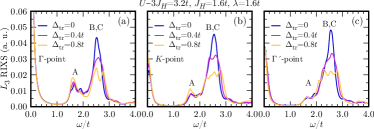
Figure S4: (Color online) The $L_{3}$-edge RIXS spectrum for $U-3J_{H}=3.2t$, $J_{H}=1.6t$, and $\lambda=1.6t$ calculated at (a) $\Gamma$, (b) $K$, and (c) $\Gamma^{\prime}$ points [see the inset of Fig. S3(b)] for three different trigonal crystal fields $\Delta_{\rm tr}$ denoted in the figure. The main peak corresponding to the local $d$-$d$ transition is split into double (or multiple) peaks (denoted as ‘B’ and ‘C’) in the presence of te trigonal distortion.

IV Local multiplet structure

It is instructive to examine the energy hierarchy of local multiplets, which is obtained simply by solving the single-site terms in Eq. (S1). Figure S5 summarizes the energy hierarchy of three relevant configurations, i.e., $d^{4}$, $d^{5}$, and $d^{6}$ electron configurations in the $t_{2g}$ manifold.

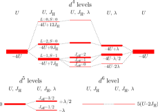
Figure S5: (Color online) Schematic energy diagrams of multiplet hierarchy in the atomic limit for three relevant electron configurations, i.e., $d^{4}$, $d^{5}$, and $d^{6}$ in the $t_{2g}$ manifold. The multiplet energy levels are represented by red lines (the width is proportional to the degeneracy) when non-zero $U$, $J_{\rm H}$, or/and $\lambda$ (indicated at the top of each diagram) are considered. The multiplet energy shown by each level is measured from the $d^{5}$ multiplet energy $E_{0}$ without the SOC.

In the case of $d^{5}$ electron configuration, only the SOC plays a role in determining the doublet ($J_{\rm eff}=1/2$) and quartet ($J_{\rm eff}=3/2$) states with their energies $E_{0}-\lambda$ and $E_{0}+\frac{\lambda}{2}$, respectively, while the Hund’s coupling $J_{\rm H}$ cannot have any effect on their multiplets. Here, $E_{0}$ is the energy for $d^{5}$ electron configuration when $\lambda=0$. Because the energy splitting between these two manifolds is $\frac{3}{2}\lambda$, the local $d$-$d$ transition, which is accessed by the RIXS, appears in this energy region.

On the contrary, in the case of $d^{4}$ electron configuration, not only $\lambda$ but also $J_{\rm H}$ determines the multiplet hierarchy. When $J_{\rm H}\neq 0$ but $\lambda=0$, fifteen-fold degenerate states split into nine-fold degenerate states with total angular moment $L=1$ and total spin momentum $S=1$, five-fold degenerate states with $L=2$ and $S=0$, and a singlet state with $L=S=0$. Their energies are, respectively, $E_{0}-4U+7J_{\rm H}$, $E_{0}-4U+9J_{\rm H}$, and $E_{0}-4U+12J_{\rm H}$, thus following the Hund’s rule. A finite $\lambda$ induces addition splittings. The lowest nine-fold degenerate states are split into $J_{\rm eff}=0$, $J_{\rm eff}=1$, and $J_{\rm eff}=2$ states. Because there are non-negligible mixing between the $J_{\rm eff}=0$ state and the singlet state with $L=S=0$, and also between the $J_{\rm eff}=2$ states and the five-fold degenerate states with $L=2$ and $S=0$, the exact energy levels for the $J_{\rm eff}=0$ and $J_{\rm eff}=2$ states are not simply expressed analytically. However, the energy difference between the lowest $J_{\rm eff}=0$ and $J_{\rm eff}=2$ states is always $\frac{3}{2}\lambda$. The energy of the $J_{\rm eff}=1$ states is instead given analytically as $E_{0}-4U+7J_{\rm H}-\frac{\lambda}{2}$. When $J_{\rm H}\gg\lambda$, the energies of the lowest $J_{\rm eff}=0$ and $J_{\rm eff}=2$ states are $E_{0}-4U+7J_{\rm H}-\lambda$ and $E_{0}-4U+7J_{\rm H}+\frac{\lambda}{2}$, respectively. In the opposite limit $\lambda\gg J_{\rm H}$, their energies are given as $E_{0}-4U+7J_{\rm H}-2\lambda$ and $E_{0}-4U+7J_{\rm H}-\frac{\lambda}{2}$, respectively.

Note that the optical excitations are determined in the multiplet theory by the energy difference between the ground state in $d^{5}d^{5}$ electron configuration and the excited states in $d^{4}d^{6}$ electron configuration. Therefore, the lowest optical peak appears at $U-3J_{\rm H}$ when $\lambda=0$. When $\lambda$ is finite, the lowest optical peaks are composed of three subpeaks. The central peak, which corresponds to the $J_{\rm eff}=1$ multiplet in the $d^{4}$ electron configuration, appears at $U-3J_{\rm H}+\frac{3\lambda}{2}$. The first (third) lowest peak, related to the $J_{\rm eff}=0$ ($J_{\rm eff}=2$) multiplet in the $d^{4}$ electron configuration, appears in an energy range between $U-3J_{\rm H}$ ($U-3J_{\rm H}+\frac{3\lambda}{2}$) and $U-3J_{\rm H}+\lambda$ ($U-3J_{\rm H}+\frac{5\lambda}{2}$), depending on the relative strength of $J_{\rm H}$ and $\lambda$. Since the hopping between the NN $j_{\rm eff}=1/2$ orbitals is absent when the hopping is mediated via the edge-sharing oxygens, the optical peak attributed to the $J_{\rm eff}=0$ multiplet in the $d^{4}$ electron configuration is diminished S (7). Contribution of the third multiplet ($J_{\rm eff}=2$) in the $d^{4}$ electron configuration is also suppressed because its optical transition amplitude between $J_{\rm eff}=1/2$ in the $d^{5}$ electron configuration and $J_{\rm eff}=2$ in the $d^{4}$ electron configuration is as small as quarter of that between $J_{\rm eff}=1/2$ in the $d^{5}$ electron configuration and $J_{\rm eff}=1$ in the $d^{4}$ electron configuration. Therefore, the honeycomb lattice system in the relativistic Mott insulating limit shows a dominant optical peak at $U-3J_{\rm H}+\frac{3\lambda}{2}$, attributed to the excitation to the $J_{\rm eff}=1$ multiplet in the $d^{4}$ electron configuration.

V Effect of direct hopping $t^{\prime}$ between neighboring $d$ orbitals

Even thought the dominant hopping process in the honeycomb lattice is via the ligand $p$ orbitals, the spatial extension of $4d$ and $5d$ orbitals is large enough to give rise to the direct hopping between neighboring TM $d$ orbitals. Recent theoretical study based on first-principles density functional calculations has estimated that the direct hopping $t^{\prime}$ between $XY$, $YZ$, and $ZX$ orbitals along the $XY$-, $YZ$-, and $ZX$-directions, respectively, can be as large as $t^{\prime}/t\approx 0.10$ for Na₂IrO₃ and $-0.97$ for $\alpha$-RuCl₃ S (9). Therefore, $t^{\prime}$ is also an important parameter in determining the electronic state specially for $\alpha$-RuCl₃.

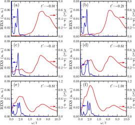
Figure S6: (Color online) OC $\sigma(\omega)$ (red lines) and $L_{3}$-edge RIXS spectrum at momentum ${\mathbf{q}}=0$ (blue lines) for various direct $d$-$d$ hoppings $t^{\prime}$ indicated in the figures for $U-3J_{\rm H}=6t$, $J_{\rm H}=1.6t$, and $\lambda=0.8t$. Here, no trigonal distortion is considered.

Figure S6 presents the OC and RIXS spectra for various values of $t^{\prime}$ when $U-3J_{\rm H}=6t$, $J_{\rm H}=1.6t$, and $\lambda=0.8t$. An interesting feature is that the low-energy optical peaks arise around $2t$ in addition to the dominant peaks with the large spectral weight near $7t$. For small $|t^{\prime}|\,(\leq 0.4t$), the small low-energy optical peaks appear near the dominant RIXS peak ($\approx 1.4t$) extended up to around the higher edge of the RIXS spectrum ($\approx 2.5t$), which is in good agreement with the experimental observations S (10, 11). Recall that the dominant RIXS peak is attributed to the local $d$-$d$ transition from the $j_{\rm eff}=3/2$ to $1/2$ orbitals. The direct hopping $t^{\prime}$ enhances the optical contribution of the electron-hole excitation between the neighboring $j_{\rm eff}=1/2$ orbitals, which is largely suppressed in the edge-shared geometry when $t^{\prime}=0$. Our results thus imply that the unusual coupling between these two different types of excitations, i.e., the electron-hole excitations between the neighboring $j_{\rm eff}=1/2$ orbitals and the local $d$-$d$ excitations, can play a role in the low-energy optical excitations. This coupling is possible because of the finite inter-band transition between the $j_{\rm eff}=1/2$ and $3/2$ bands S (7).

For large $|t^{\prime}|\,(\geq 0.6t)$, we find in Fig. S6 that a large amount of spectral weights in the OC are transferred from the high-energy region ($\gtrsim 4t$) to the low-energy region ($\lesssim 4t$). This observation with a large amount of low-energy spectral weight is far from the experimental observations S (10, 11) and thus indicates that the first-principles density functional calculations overestimate $|t^{\prime}|$ S (9).

References

- (1) B. J. Kim, H. Jin, S. J. Moon, J.-Y. Kim, B.-G. Park, C. S. Leem, J. Yu, T. W. Noh, C. Kim, S.-J. Oh, J.-H. Park, V. Durairaj, G. Cao, and E. Rotenberg, Phys. Rev. Lett. 101, 076402 (2008).
- (2) B. J. Kim, H. Ohsumi, T. Komesu, S. Sakai, T. Morita, H. Takagi, and T. Arima, Science 323, 1329 (2009).
- (3) G. Jackeli and G. Khaliullin, Phys. Rev. Lett. 102, 017205 (2009).
- (4) H. Watanabe, T. Shirakawa, and S. Yunoki, Phys. Rev. Lett. 105, 216410 (2010).
- (5) C. Martins, M. Aichhorn, L. Vaugier, and S. Biermann, Phys. Rev. Lett. 107, 266404 (2011).
- (6) F. Wang and T. Senthil, Phys. Rev. Lett. 106, 136402 (2011).
- (7) H. Watanabe, T. Shirakawa, and S. Yunoki, Phys. Rev. Lett. 110, 027002 (2013).
- (8) D. Pesin and L. Balents, Nature Phys. 6, 376 (2010).
- (9) B.-J. Yang and Y. B. Kim, Phys. Rev. B 82, 085111 (2010).
- (10) W. Witczak-Krempa and Y. B. Kim, Phys. Rev. B 85, 045124 (2012).
- (11) A. Go, W. Witczak-Krempa, G. S. Jeon, K. Park, and Y. B. Kim, Phys. Rev. Lett. 109, 066401 (2012).
- (12) Y. Okamoto, M. Nohara, H. Aruga-Katori, and H. Takagi, Phys. Rev. Lett. 99, 137207 (2007).
- (13) Y. Singh, Y. Tokiwa, J. Dong, and P. Gegenwart, Phys. Rev. B 88, 220413(R) (2013).
- (14) A. Shitade, H. Katsura, J. Kuneš, X.-L. Qi, S.-C. Zhang, and N. Nagaosa, Phys. Rev. Lett. 102, 256403 (2009).
- (15) C. H. Kim, H. S. Kim, H. Jeong, H. Jin, and J. Yu, Phys. Rev. Lett. 108, 106401 (2012).
- (16) J. Chaloupka, G. Jackeli, and G. Khaliullin, Phys. Rev. Lett. 105, 027204 (2010).
- (17) H.-C. Jiang, Z.-C. Gu, X.-L. Qi, and S. Trebst, Phys. Rev. B 83, 245104 (2011).
- (18) J. Reuther, R. Thomale, and S. Trebst, Phys. Rev. B 84, 100406(R) (2011).
- (19) Y. Singh and P. Gegenwart, Phys. Rev. B 82, 064412 (2010).
- (20) X. Liu, T. Berlijn, W.-G. Yin, W. Ku, A. Tsvelik, Y.-J. Kim, H. Gretarsson, Y. Singh, P. Gegenwart, and J. P. Hill, Phys. Rev. B 83, 220403(R) (2011).
- (21) S. K. Choi, R. Coldea, A. N. Kolmogorov, T. Lancaster, I. I. Mazin, S. J. Blundell, P. G. Radaelli, Y. Singh, P. Gegenwart, K. R. Choi, S.-W. Cheong, P.J. Baker, C. Stock, and J. Taylor, Phys. Rev. Lett. 108, 127204 (2012).
- (22) F. Ye, S. Chi, H. Cao, B. C. Chakoumakos, J. A. Fernandez-Baca, R. Custelcean, T. F. Qi, O. B. Korneta, and G. Cao, Phys. Rev. B 85, 180403(R) (2012).
- (23) Y. Singh, S. Manni, J. Reuther, T. Berlijn, R. Thomale, W. Ku, S. Trebst, and P. Gegenwart, Phys. Rev. Lett. 108, 127203 (2012).
- (24) Y. Luo, C. Cao, B. Si, Y. Li, J. Bao, H. Guo, X. Yang, C. Shen, C. Feng, J. Dai, G. Cao, and Z.-a. Xu, Phys. Rev. B 87, 161121(R) (2013).
- (25) J. A. Sears, M. Songvilay, K. W. Plumb, J. P. Clancy, Y. Qiu, Y. Zhao, D. Parshall, and Y.-J. Kim, Phys. Rev B 91, 144420 (2015).
- (26) M. Majumder, M. Schmidt, H. Rosner, A. A. Tsirlin, H. Yasuoka, and M. Baenitz, Phys. Rev B 91, 180401(R) (2015).
- (27) R. D. Johnson, S. C. Williams, A. A. Haghighirad, J. Singleton, V. Zapf, P. Manuel, I. I. Mazin, Y. Li, H. O. Jeschke, R. Valentí, and R. Coldea, Phys. Rev. B 92, 235119 (2015).
- (28) R. Comin, G. Levy, B. Ludbrook, Z.-H. Zhu, C. N. Veenstra, J. A. Rosen, Y. Singh, P. Gegenwart, D. Stricker, J. N. Hancock, D. van der Marel, I. S. Elfimov, and A. Damascelli, Phys. Rev. Lett. 109, 266406 (2012).
- (29) H. Gretarsson, J. P. Clancy, X. Liu, J. P. Hill, E. Bozin, Y. Singh, S. Manni, P. Gegenwart, J. Kim, A. H. Said, D. Casa, T. Gog, M. H. Upton, H.-S. Kim, J. Yu, V. M. Katukuri, L. Hozoi, J. van den Brink, and Y.-J. Kim, Phys. Rev. Lett 110, 076402 (2013).
- (30) C. H. Sohn, H.-S. Kim, T. F. Qi, D. W. Jeong, H. J. Park, H. K. Yoo, H. H. Kim, J.-Y. Kim, T. D. Kang, D.-Y. Cho, G. Cao, J. Yu, S. J. Moon, and T. W. Noh, Phys. Rev. B 88, 085125 (2013).
- (31) B. H. Kim, G. Khaliullin, and B. I. Min, Phys. Rev. B 89, 081109(R) (2014).
- (32) K. W. Plumb, J. P. Clancy, L. J. Sandilands, V. V. Shankar, Y. F. Hu, K. S. Burch, H.-Y. Kee, and Y.-J. Kim, Phys. Rev. B 90, 041112(R) (2014).
- (33) H.-S. Kim, Vijay Shankar V., A. Catuneanu, and H.-Y. Kee, Phys. Rev. B 91, 241110(R) (2015).
- (34) I. Kimchi and Y.-Z. You, Phys. Rev. B 84, 180407(R) (2011).
- (35) J. Chaloupka, G. Jackeli, and G. Khaliullin, Phys. Rev. Lett. 110, 097204 (2013).
- (36) I. I. Mazin, H. O. Jeschke, K. Foyevtsova, R. Valentí, and D. I. Khomskii, Phys. Rev. Lett. 109, 197201 (2012).
- (37) I. I. Mazin, S. Manni, K. Foyevtsova, H. O. Jeschke, P. Gegenwart, and R. Valentí, Phys. Rev. B 88, 035115 (2013).
- (38) K. Foyevtsova, H. O. Jeschke, I. I. Mazin, D. I. Khomskii, and R. Valentí, Phys. Rev. B 88, 035107 (2013).
- (39) H.-J. Kim, J.-H. Lee, and J.-H. Cho, Sci. Rep. 4, 5253 (2014).
- (40) Y. Li, K. Foyevtsova, H. O. Jeschke, and R. Valentí, Phys. Rev. B 91, 161101(R) (2015).
- (41) M. Kim, B. H. Kim, and B. I. Min, Phys. Rev. B 93, 195135 (2016).
- (42) J.-i. Igarashi and T. Nagao, J. Phys.: Condens. Matter 28, 026006 (2016).
- (43) See Supplemental Material for the detailed Hamiltonian, quasimolecular bands, cluster calculation of , , OC and RIXS spectra, local multiplet structures, and the effect of the direct hopping on OC and RIXS spectra, which also includes Refs. Kanamori63 ; Ament11 ; Chun2015 .
- (44) J. Kanamori, Prog. Theor. Phys. 30, 275 (1963).
- (45) L. J. P. Ament, M. van Veenendaal, T. P. Devereaux, J. P. Hill, and J. van den Brink, Rev. Mod. Phys. 83, 705 (2011).
- (46) S. H. Chun, J.-W. Kim, J. Kim, H. Zheng, C. C. Stoumpos, C. D. Malliakas, J. F. Mitchell, K. Mehlawat, Y. Singh, Y. Choi, T. Gog, A. Al-Zein, M. M. Sala, M. Krisch, J. Chaloupka, G. Jackeli, G. Khaliullin, and B. J. Kim, Nature Phys. 11, 462 (2015).
- (47) R. B. Morgan and D. S. Scott, SIAM J. Sci. Comput. 14, 585 (1993).
- (48) E. Dagotto, Rev. Mod. Phys. 66, 763 (1994).
- (49) Let and be the nearest neighbor hoppings between and orbitals, and between orbitals, respectively, along the -direction. One can show that the nearest neighbor hopping between orbitals with the same isospin is . Therefore, there is no optical transition among the pure bands when .
- (50) D. Dai, H. J. Xiang, and M.-H. Whangbo, J. Comput. Chem. 29, 2187 (2008).
- (51) J. P. Clancy, N. Chen, C. Y. Kim, W. F. Chen, K. W. Plumb, B. C. Jeon, T. W. Noh, and Y.-J. Kim, Phys. Rev. B 86, 195131 (2012).
- (52) Y. Yamaji, Y. Nomura, M. Kurita, R. Arita, and M. Imada, Phys. Rev. Lett. 113, 107201 (2014).
- (53) S. M. Winter, Y. Li, H. O. Jeschke, and R. Valentí, Phys. Rev. B 93, 214431 (2016).
- (54) The trigonal crystal field splitting among orbitals is estimated as large as 75 meV in Ref. Foyevtsova2013 .
- (55) X. Liu, Vamshi M. Katukuri, L. Hozoi, W.-G. Yin, M. P. M. Dean, M. H. Upton, J. Kim, D. Casa, A. Said, T. Gog, T. F. Qi, G. Cao, A. M. Tsvelik, J. van den Brink, and J. P. Hill, Phys. Rev. Lett. 109, 157401 (2012).
- (56) E. M. Plotnikova, M. Daghofer, J. van den Brink, and K. Wohlfeld, Phys. Rev. Lett. 116, 106401 (2016).
- (57) L. J. Sandilands, Y. Tian, A. A. Reijnders, H.-S. Kim, K. W. Plumb, Y.-J. Kim, H.-Y. Kee, and K. S. Burch, Phys. Rev. B 93, 075144 (2016).
- (58) A. Koitzsch, C. Habenicht, E. Müller, M. Knupfer, B. Büchner, H. C. Kandpal, J. van den Brink, D. Nowak, A. Isaeva, and Th. Doert, Phys. Rev. Lett. 117, 126403 (2016).
- (59) A. Banerjee, C. A. Bridges, J.-Q. Yan, A. A. Aczel, L. Li, M. B. Stone, G. E. Granroth, M. D. Lumsden, Y. Yiu, J. Knolle, S. Bhattacharjee, D. L. Kovrizhin, R. Moessner, D. A. Tennant, D. G. Mandrus, and S. E. Nagler, Nat. Mater. 15, 733 (2016)
- (60) In Ref. Sandilands2016 , the small low-energy peak near 0.3 eV is attributed to an optically forbidden local - transition from the bands to the bands through electron-phonon coupling. However, our result supports that the pure electronic transition within the manifold can give rise to the low-energy optical excitations.
Supplementary Materials

References

- S (1) J. Kanamori, Prog. Theor. Phys. 30, 275 (1963).
- S (2) R. B. Morgan and D. S. Scott, SIAM J. Sci. Comput. 14, 585 (1993).
- S (3) E. Dagotto, Rev. Mod. Phys. 66, 763 (1994).
- S (4) L. J. P. Ament, M. van Veenendaal, T. P. Devereaux, J. P. Hill, and J. van den Brink, Rev. Mod. Phys. 83, 705 (2011).
- S (5) S. H. Chun, J.-W. Kim, J. Kim, H. Zheng, C. C. Stoumpos, C. D. Malliakas, J. F. Mitchell, K. Mehlawat, Y. Singh, Y. Choi, T. Gog, A. Al-Zein, M. M. Sala, M. Krisch, J. Chaloupka, G. Jackeli, G. Khaliullin, and B. J. Kim, Nature Phys. 11, 462 (2015).
- S (6) H. Gretarsson, J. P. Clancy, X. Liu, J. P. Hill, E. Bozin, Y. Singh, S. Manni, P. Gegenwart, J. Kim, A. H. Said, D. Casa, T. Gog, M. H. Upton, H.-S. Kim, J. Yu, V. M. Katukuri, L. Hozoi, J. van den Brink, and Y.-J. Kim, Phys. Rev. Lett 110, 076402 (2013).
- S (7) B. H. Kim, G. Khaliullin, and B. I. Min, Phys. Rev. B 89, 081109(R) (2014).
- S (8) K. Foyevtsova, H. O. Jeschke, I. I. Mazin, D. I. Khomskii, and R. Valentí, Phys. Rev. B 88, 035107 (2013).
- S (9) S. M. Winter, Y. Li, H. O. Jeschke, and R. Valentí, Phys. Rev. B 93, 214431 (2016).
- S (10) K. W. Plumb, J. P. Clancy, L. J. Sandilands, V. V. Shankar, Y. F. Hu, K. S. Burch, H.-Y. Kee, and Y.-J. Kim, Phys. Rev. B 90, 041112(R) (2014).
- S (11) L. J. Sandilands, Y. Tian, A. A. Reijnders, H.-S. Kim, K. W. Plumb, Y.-J. Kim, H.-Y. Kee, and K. S. Burch, Phys. Rev. B 93, 075144 (2016).