Prisoner’s dilemma on directed networks

Abstract

We study the prisoner’s dilemma model with a noisy imitation evolutionary dynamics on directed out-homogeneous and uncorrelated directed random networks. An heterogeneous pair mean-field approximation is presented showing good agreement with Monte Carlo simulations in the limit of weak selection (high noise) where we obtain analytical predictions for the critical temptations. We discuss the phase diagram as a function of temptation, intensity of noise and coordination number of the networks and we consider both the model with and without self-interaction. We compare our results with available results for non-directed lattices and networks.

1 Introduction

Dilemmas arise when it is advantageous for an individual to act selfishly by not taking into account the overall performance of the group it belongs to[1, 2, 3, 4]. Such dilemmas can be modeled by simple two agent games where each agent follows two strategies, cooperation (C) and defection (D) and receive a payoff after each round that depends on the chosen strategy. In the prisoners dilemma game[5, 6] (PD) a defector facing a cooperator receives the highest payoff (T- temptation) higher than the second best payoff (R- reward) received from mutual cooperation. The smallest payoff is received by a cooperator facing a defector (S - sucker payoff), even smaller than the payoff received from mutual defection (P- punishment). In a population of defectors, an agent does not increase it’s payoff by changing it’s strategy to cooperation contrary to the case of a population of cooperators where it is advantageous for an agent to change to defection. Defection is the best reply to defection which classifies this strategy as a Nash equilibrium in a game theory framework[2]. However, cooperation is observed in social and biological systems even when from an agent point of view it is better not to cooperate. Evolutionary games are obtained when the best strategies become more frequent by giving a higher reproductive ability to agents following those strategies. Several mechanisms for the evolution of cooperation were proposed, some of them relying on strategies that assume repeated encounters and some sort of memory [7].

Considering only pure strategies (C and D), it was found that the introduction of a spatial or a network structure in the population [8, 9, 10, 11, 12] where an agent plays with nearest neighbors (possibly including itself) and receives a total payoff collected from each of those two agent games can lead to the emergence of cooperation.

The PD game has been studied in structured populations such as lattices[8, 9, 10, 13, 14], hierarchical lattices[15], empirical social networks[16], small world networks[17, 18, 19, 20, 21, 22, 23], homogeneous random networks[24], single scale [25, 23] and scale-free networks[22, 26, 25, 27, 23]. In the case of well mixed populations and fully connected networks where the payoff of each agent depends directly on the frequency of each strategy in the whole population the PD model evolves to a phase where all agents are defectors. The clustering of cooperators in a spatial/network structure allows cooperators to resist exploitation and the population may evolve to a coexistence phase of cooperators and defectors[28]. Structural heterogeneity in the number of neighbors was found to favor generically cooperation in the PD game [21, 7, 25, 27] although this effect may depend on the details of the adopted evolutionary rule [3, 29].

The distinction between the lattice/network of interactions where the agents play and the lattice/network of influence where the learning and reproduction process takes place[30, 31, 32] was previously introduced. In those studies both the network of interactions and the network of influences was considered to be non-directed. The influence between agents in empirical social networks is sometimes found to be asymmetric and requiring modeling by directed networks[33]. This asymmetry may be taken into account in the framework of evolving networks by considering time evolving weights which depend on the outcome of ongoing interactions between the agents[34, 3, 35, 36] .

In this work we study the PD model in the case where the network of interactions and the network of learning are identical directed networks. Specifically, we consider that when an agent A plays with it’s neighbor agent B ( which does not have A as its own neighbor) only A collects the payoff for the game between them. Even though the PD game is a two agent game the payoffs (consequences) of the adopted strategies (actions) may be collected asymmetrically by the two players engaged in a particular interaction. In previous works the case of a single influential node with long-range asymmetric interactions was considered[18] and the evolutionary dynamics on a directed cycle (one dimensional directed lattice) where the payoffs of the two agent games are collected asymmetrically was discussed[37].

Several techniques were used to study two player game models on spatial structures such as Monte Carlo simulation, calculations of the probability of fixation of mutant strategies[28] and the determination of the evolutionary stable strategies by deriving an effective replicator dynamics[38, 39]. The last two techniques assume the limit of weak selection and rely on mean-field (MF) pair approximation. [13, 3]. Unless in conditions of weak selection, higher order cluster MF approximations[13, 24, 3], going beyond the pair approximation, are usually needed to obtain accurate results. Such higher order approximations were applied before to model dynamical processes in regular lattices[40, 41, 13, 3] and networks with an homogeneous degree structure[42]. In directed lattices with a local tree like structure single-site MF approximations may give surprisingly accurate results[43]. In this work, we present an heterogeneous single-site and pair MF approximation for the PD game on a generic directed network taking into account the degree heterogeneities and degree correlations. In general, there is no unique way of deriving mean-field approximations from the master equation describing dynamical processes in the networks[44, 45]. Our approach is close in spirit to the annealed mean-field approximations previously used to study epidemic spreading in heterogeneous networks[46, 47].

The remaining of the paper is organized as follows: in section 2 we describe in detail the version of the PD model and the networks considered; in section 3 we present our single-site and pair MF approximations; in section 4 the results obtained for out-homogeneous directed networks of different out-degree are presented; in section 5 we compare the predictions of the pair approximation with Monte Carlo simulation for the steady-state density of cooperators in Poissonian random directed networks and finally in section 6 we summarize our main conclusions.

2 the model on directed random networks

We consider a scaled version of the payoff matrix of the PD model [8, 13] where the reward payoff for mutual cooperation is set to unity, the temptation payoff received by a $D$ facing a $C$ is $b$ and all other payoffs are null. The dilemma strictly exists for $b>1$ when defecting becomes advantageous from the individual point of view. When the game is played on a network, at each vertex, $i$ , there is an agent that receives a total payoff, $P_{i}$, that depends on the strategies adopted by the neighbors. We study in more detail the case where self-interaction is included and the payoff for a $C$ is then equal to $n_{C}+1$ and the payoff for a $D$ is equal to $b\,n_{C}$, being $n_{C}$ the number of neighbors that follow the strategy $C$. The inclusion of self-interaction may be justified by seeing each agent as representing a group following a given strategy[8] in a coarse-grained sense. Unless explicitly mentioned the results presented are for the model with self-interaction. For a network with $N$ vertices, where a vertex $i$ has $k_{i}$ neighbors, an imitation dynamics is considered such that a randomly chosen agent, $i,\,1\leq i\leq N$ chooses a random neighbor, $i_{\mu},1\leq\mu\leq k_{i}$, and if this neighbor is following a different strategy it adopts the strategy of the neighbor with probability

$$p_{\mathrm{imitate}}(P_{i},P_{i_{\mu}})=\frac{1}{1+\exp\left(-\beta\left(P_{i_{\mu}}-P_{i}\right)\right)},$$ (1)

where $T=\beta^{-1}$ is a temperature like parameter that controls the level of noise in the strategy imitation process. The weak selection limit corresponds to large $T$ when the dependence of the imitation probability on the agent’s payoff difference is small and linear. The above imitation dynamics[13] is sometimes called pairwise comparison dynamics and it is just one of several possible reasonable evolutionary dynamics [48]. In a system where each agent has $z$ neighbors the total payoff of the full cooperation phase would be $N\left(z+1\right)$ and an alternating phase where each $C$ is surrounded by $D$ and vice-versa, if possible, would have a total system payoff $Nbz/2+N/2$. Thus only for $b<2+1/z$ ($b<2$ without self-interaction) the full cooperation phase corresponds to the maximum system payoff but, for any value of $b$, the full defection phase is always the phase with the smallest system payoff. In a large fully connected network the density of cooperators $\rho(t)$ can be written as $d\rho/dt=\rho\left(1-\rho\right)\tanh\left(\beta\rho(1-b)\right)$ which, in the limit of weak selection, has the replicator equation form [2, 4] with a solution that reaches zero for long times, when $b>1$.

We study the model on two kinds of directed random networks where the neighbors of a vertex are connected through outgoing links starting from a vertex. In the directed out-homogeneous networks[49, 43] the number of out-links, $z$, is the same for all vertices. The out-links are generated by selecting randomly, for each vertex of the network, $z$ other (different) vertices. The distribution of in-links is Poissonian as for random networks. For $z>1$ the system is in a percolating phase with a giant strongly connected component containing a finite fraction of the vertices[43]. The other kind of networks considered are directed random networks which are built by establishing an outgoing link, $i\rightarrow j$ , from each vertex, $i$, to each other vertex, $j$ with probability $q/N$. The distribution of the number of outgoing links of a given vertex as well as the distribution of the number of ingoing links is Poissonian with an average value $q.$ For these networks, vertices with no out-links (without neighbors) may receive an arbitrary number of in-links, thus influencing other vertices, while their own strategies do not suffer influence from others. To avoid this behavior we generated the out-links starting from a truncated and renormalized Poisson distribution where vertices with no out-going links have zero probability. The average number of out-links of a vertex is then $z=\left\langle k_{\mathrm{out}}\right\rangle=\tfrac{q}{1-\exp(-q)}$, always larger than unity. To generate these networks we use a method based on the configuration model[50]: the out-degrees of each vertex, $i$, are drawn from its probability distribution, thus generating $k_{i}$ stubs which are ends of outgoing links emerging from the vertex $i$. These stubs are then connected to randomly chosen vertices with the restriction of not repeating a vertex and not allowing connections to itself.

The directed networks[51, 52, 53] are characterized by a joint in-degree and out-degre distribution, $P\left(k_{\mathrm{i\mathrm{n}}},k_{\mathrm{out}}\right)$ and degree correlations $P_{\mathrm{i\mathrm{n}}}\left(k^{\prime}_{\mathrm{in}},k^{\prime}_{\mathrm{out}}|k{}_{\mathrm{in}},k_{\mathrm{out}}\right)$ and $P_{\mathrm{out}}\left(k^{\prime}_{\mathrm{in}},k^{\prime}_{\mathrm{out}}|k{}_{\mathrm{in}},k_{\mathrm{out}}\right)$, which measure the probability to reach a vertex of degrees $k^{\prime}_{\mathrm{in}}\mathrm{\,and\,}k^{\prime}_{\mathrm{out}}$ from a vertex of degrees $k{}_{\mathrm{in}}\mathrm{\,and\,}k{}_{\mathrm{out}}$ following, respectively, an in-link and an out-link. For the particular case of networks with uncorrelated in-degre and out-degree, $P\left(k_{\mathrm{in}},k_{\mathrm{out}}\right)=P_{\mathrm{in}}(k_{\mathrm{in}})P_{\mathrm{out}}(k_{\mathrm{out}})$ and with uncorrelated degree vertices, such that $P_{\mathrm{i\mathrm{n}}}\left(k^{\prime}_{\mathrm{in}},k^{\prime}_{\mathrm{out}}|k{}_{\mathrm{in}},k_{\mathrm{out}}\right)$ and $P_{\mathrm{out}}\left(k^{\prime}_{\mathrm{in}},k^{\prime}_{\mathrm{out}}|k{}_{\mathrm{in}},k_{\mathrm{out}}\right)$ are independent of $k{}_{\mathrm{i\mathrm{n}}}\mathrm{\,and\,}k{}_{\mathrm{out}}$ , it can be shown, from a detailed balance relation [53], that:

$$P_{\mathrm{out}}\left(k^{\prime}_{\mathrm{out}}|k_{\mathrm{out}}\right)=P_{\mathrm{out}}(k^{\prime}_{\mathrm{out}}).$$ (2)

The random networks considered in this work are uncorrelated in the sense defined above.

3 Mean Field Theory

We derived an heterogeneous single-site and pair mean-field theory for the model on a directed network characterized by an out-link degree-degree correlation $P_{\mathrm{out}}\left(k^{\prime}_{\mathrm{out}}|k_{\mathrm{out}}\right)$. Our approach can be easily applied to other network dynamic models. The single-site approximation time evolution equation for the probability $p_{k}(C,t)=1-p_{k}(D,t)$ to have a cooperator at a vertex of an out-degree $k$, at time $t$, is:

$$\frac{d}{dt}p_{k}(C,t)=R_{1}\,\left(1-p_{k}(C,t)\right)-R_{2}\,p_{k}(C,t).$$ (3)

The processes that contribute to the time evolution equation are listed in Table 1. The summations in the rates, $R_{i}$ are over the possible out-degree values of the neighboring vertices of a given vertex and the average of the imitation probability over the possible neighborhoods of the vertex and of the neighboring vertices are taken from binomial distributions, $B_{m}(x)$ where $m$ is the number of attempts (number of neighbors taken into the average) and $x$ is the success probability of each attempt obtained from the probability to find a $C$ at a neighboring vertex of a vertex of a given degree, $k$, at time $t$, $\rho_{k}^{(n)}(t)$ that can be written as, $\rho_{k}^{(n)}(t)={\textstyle\sum_{m}p_{m}(C,t)P_{\mathrm{out}}(m|k)}$. Note that for a degree-degree uncorrelated network this quantity does not depend on the out-degree $k$.

i	process	rate, $R_{i}$	n-dist	l-dist
1	${}_{\cdots\leftarrow D_{k}\rightarrow C_{s}\rightarrow\cdots}$	${}_{\sum_{s}p_{s}(C,t)P_{\mathtt{out}}(s|k)\,\left\langle p_{\mathtt{imitate}}\left(b\left(n+1\right),l+1\right)\right\rangle}$	${}_{B_{k-1}\left(\rho_{k}^{(n)}(t)\right)}$	${}_{B_{s}\left(\rho_{s}^{(n)}(t)\right)}$
2	${}_{\cdots\leftarrow C_{k}\rightarrow D_{s}\rightarrow\cdots}$	${}_{\sum_{s}\left(1-p_{s}(C,t)\right)P_{\mathtt{out}}(s|k)\,\left\langle p_{\mathtt{imitate}}\left(n+1,b\,l\right)\right\rangle}$	${}_{B_{k-1}\left(\rho_{k}^{(n)}(t)\right)}$	${}_{B_{s}\left(\rho_{s}^{(n)}(t)\right)}$

Table 1: Processes and corresponding rates for the single site mean-field approximation for the model with self-interaction. The quantities $B_{m}\left(x\right)$ represent the Binomial distribution with $m$ attempts and success probability, $x$.

The processes that contribute to the pair approximation are listed in Table 2. The time evolution equations for the probabilities, $p_{k,m}(XY,t)$ for a vertex with out-degree $k$ to follow strategy $X=C,D$ and for a neighbor of that vertex, with out-degree $m$, to follow strategy $Y=C,D$, at time $t$, are given by:

$$\begin{array}[]{lll}\frac{d}{dt}p_{k,m}\left(CC,t\right)&=&\left(R_{1}+R_{2}\right)\,p_{k,m}\left(DC,t\right)+R_{3}\,p_{k,m}\left(CD,t\right)\\ &&\qquad\qquad-\left(R_{4}+R_{5}\right)\,p_{k,m}\left(CC,t\right)\\ \frac{d}{dt}p_{k,m}\left(CD,t\right)&=&R_{10}\,p_{k,m}\left(DD,t\right)+R_{5}\,p_{k,m}\left(CC,t\right)\\ &&\qquad\qquad-\left(R_{3}+R_{8}+R_{9}\right)\,p_{k,m}\left(CD,t\right)\\ \frac{d}{dt}p_{k,m}\left(DC,t\right)&=&R_{4}\,p_{k,m}\left(CC,t\right)+R_{6}\,p_{k,m}\left(DD,t\right)\\ &&\qquad\qquad-\left(R_{1}+R_{2}+R_{7}\right)\,p_{k,m}\left(DC,t\right)\\ \frac{d}{dt}p_{k,m}\left(DD,t\right)&=&\left(R_{8}+R_{9}\right)\,p_{k,m}\left(CD,t\right)+R_{7}\,p_{k,m}\left(DC,t\right)\\ &&\qquad\qquad-\left(R_{10}+R_{6}\right)\,p_{k,m}(DD,t)\end{array}$$ (4)

The averages of the imitation probabilities, included in Table 2, are taken from binomial distributions, as in the single-site approximation case, with a success probability given by the conditional probability, $\rho_{k}^{(n)}(X,t)$ to find a $C$ at a vertex neighbor to a vertex of out-degree $k$ given that the agent at this vertex is following strategy $X=C,D$. This quantity can be written as:

$$\rho_{k}^{(n)}(X,t)={\textstyle\sum_{m}\frac{p_{k,m}(XC,t)}{p_{k,m}^{(1)}(X,t)}P_{\mathrm{out}}\left(m|k\right)}$$ (5)

where $p_{k,m}^{(1)}(X,t)=p_{k,m}(XC,t)+p_{k,m}(XD,t)$ .

The density of cooperators, $\rho(t)$, is obtained, in the pair approximation, from:

$$\rho(t)=\sum_{k,m}p_{k,m}^{(1)}(C,t)P_{\mathrm{out}}(m|k)\,P_{\mathrm{out}}(k)$$

In the derivation of the pair approximation, probabilities of configurations of more than two out-linked vertices are approximated by probabilities of configurations of pairs of out-linked vertices in the spirit of the probability approximation methods previously applied to dynamical models on regular lattices [41, 40, 13, 3] .

i	process	rate, $R_{i}$	n-dist	l-dist
1	${}_{\cdots\leftarrow D_{k}\rightarrow C_{m}\rightarrow\cdots}$	${}_{\frac{1}{k}\left\langle p_{\mathtt{imitate}}\left(b\left(n+1\right),l+1\right)\right\rangle}$	${}_{B_{k-1}\left(\rho_{k}^{(n)}(D,t)\right)}$	${}_{B_{m}\left(\rho_{m}^{(n)}(C,t)\right)}$
2	$\cdots\leftarrow_{\begin{array}[]{c}C_{s}\nwarrow\\ \ldots\swarrow\end{array}D_{k}\rightarrow C_{m}}$	${}_{\frac{k-1}{k}\sum_{s}\frac{p_{k,s}(DC,t)}{p_{k,s}^{(1)}(D,t)}P_{\mathtt{out}}(s|k)\,\left\langle p_{\mathtt{imitate}}\left(b\left(n+2\right),l+1\right)\right\rangle}$	${}_{B_{k-2}\left(\rho_{k}^{(n)}(D,t)\right)}$	${}_{B_{s}\left(\rho_{s}^{(n)}(C,t)\right)}$
3	${}_{C_{k}\rightarrow D_{m}\begin{array}[]{l}\nearrow C_{s}\rightarrow\cdots\\ \searrow\ldots\end{array}}$	${}_{\sum_{s}\frac{p_{m,s}(DC,t)}{p_{m,s}^{(1)}(D,t)}P_{\mathtt{out}}(s|m)\,\left\langle p_{\mathtt{imitate}}\left(b\left(n+1\right),l+1\right)\right\rangle}$	${}_{B_{m-1}\left(\rho_{m}^{(n)}(D,t)\right)}$	${}_{B_{s}\left(\rho_{s}^{(n)}(C,t)\right)}$
4	$\cdots\leftarrow_{\begin{array}[]{c}D_{s}\nwarrow\\ \ldots\swarrow\end{array}C_{k}\rightarrow C_{m}}$	${}_{\frac{k-1}{k}\sum_{s}\frac{p_{k,s}(CD,t)}{p_{k,s}^{(1)}(C,t)}P_{\mathtt{out}}(s|k)\,\left\langle p_{\mathtt{imitate}}\left(n+2,b\,l\right)\right\rangle}$	${}_{B_{k-2}\left(\rho_{k}^{(n)}(C,t)\right)}$	${}_{B_{s}\left(\rho_{s}^{(n)}(D,t)\right)}$
5	${}_{C_{k}\rightarrow C_{m}\begin{array}[]{l}\nearrow D_{s}\rightarrow\cdots\\ \searrow\ldots\end{array}}$	${}_{\sum_{s}\frac{p_{m,s}(CD,t)}{p_{m,s}^{(1)}(C,t)}P_{\mathtt{out}}(s|m)\,\left\langle p_{\mathtt{imitate}}\left(n+1,b\,l\right)\right\rangle}$	${}_{B_{m-1}\left(\rho_{m}^{(n)}(C,t)\right)}$	${}_{B_{s}\left(\rho_{s}^{(n)}(D,t)\right)}$
6	${}_{D_{k}\rightarrow D_{m}\begin{array}[]{l}\nearrow C_{s}\rightarrow\cdots\\ \searrow\ldots\end{array}}$	${}_{R_{3}}$
7	${}_{D_{k}\rightarrow C_{m}\begin{array}[]{l}\nearrow D_{s}\rightarrow\cdots\\ \searrow\ldots\end{array}}$	${}_{R_{5}}$
8	${}_{\cdots\leftarrow C_{k}\rightarrow D_{m}\rightarrow\cdots}$	${}_{\frac{1}{k}\left\langle p_{\mathtt{imitate}}\left(n+1,b\,l\right)\right\rangle}$	${}_{B_{k-1}\left(\rho_{k}^{(n)}(C,t)\right)}$	${}_{B_{m}\left(\rho_{m}^{(n)}(D,t)\right)}$
9	$\cdots\leftarrow_{\begin{array}[]{c}D_{s}\nwarrow\\ \ldots\swarrow\end{array}C_{k}\rightarrow D_{m}}$	${}_{\frac{k-1}{k}\sum_{s}\frac{p_{k,s}(CD,t)}{p_{k,s}^{(1)}(C,t)}P_{\mathtt{out}}(s|k)\,\left\langle p_{\mathtt{imitate}}\left(n+1,b\,l\right)\right\rangle}$	${}_{B_{k-2}\left(\rho_{k}^{(n)}(C,t)\right)}$	${}_{B_{s}\left(\rho_{s}^{(n)}(D,t)\right)}$
10	$\cdots\leftarrow_{\begin{array}[]{c}C_{s}\nwarrow\\ \ldots\swarrow\end{array}D_{k}\rightarrow D_{m}}$	${}_{\frac{k-1}{k}\sum_{s}\frac{p_{k,s}(DC,t)}{p_{k,s}^{(1)}(D,t)}P_{\mathtt{out}}(s|k)\,\left\langle p_{\mathtt{imitate}}\left(b\left(n+1\right),l+1\right)\right\rangle}$	${}_{B_{k-2}\left(\rho_{k}^{(n)}(D,t)\right)}$	${}_{B_{s}\left(\rho_{s}^{(n)}(C,t)\right)}$

Table 2: Processes and corresponding rates for the pair mean-field approximation for the model with self-interaction. The quantities $B_{m}\left(x\right)$ represent the Binomial distribution as in Table 1.

4 out-homogeneous directed network

We studied the phase diagram of the prisoner’s dilemma model in the out-homogeneous networks using the mean-field approximations and Monte Carlo simulations. The model exhibits, generically, at lower temptation $b_{c,1}$, a phase transition from a full cooperation phase to an intermediate active phase, where both strategies survive, and, at higher temptation, $b_{c,2}$, a phase transition to a full defection state. The comparison of the mean-field results with simulations shows that the single-site approximation is not able to describe correctly the model and that the pair approximation gives a much better agreement with simulation.

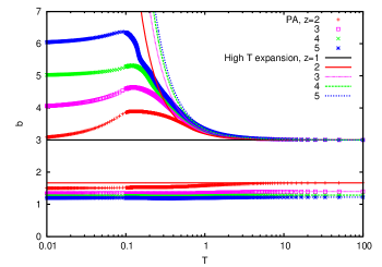
Figure 1: Phase diagrams in the pair approximation (PA) for the out-homogeneous networks with $z=2,3,4$ and $5$. The lower curves are $b_{c,1}$ and the upper curves are $b_{c,2}$. The lines are the high temperature expansion results presented in Eq. (6).

4.1 mean-field approximations

From a high temperature expansion we were able to obtain analytical results for the transition parameters, $b_{c,1}$and $b_{c,2}$ for a network with an arbitrary number of outgoing neighbors, $z$. For the single-site approximation we obtained $b_{c,1}=\tfrac{2z+1}{2z}$ and $b_{c,2}=2$, and for the pair approximation:

$$\begin{array}[]{cl}b_{c,1}&=\frac{2z+1}{2z-1}\\ b_{c,2}&=3+\frac{1}{T}\,\frac{\left(z-1\right)^{2}}{\left(2z-1\right)^{2}}\end{array}.$$ (6)

We also applied the method proposed in Ref. [54] to numerically study the MF phase diagram in the temptation and temperature parameters space. The rate of the time evolution of the density of cooperators in the equation $\frac{d\rho}{dt}=F(\rho)$ was obtained by solving, for each $\rho$, a set of modified dynamical equations that conserve $\rho$:

$$\begin{array}[]{ccc}\frac{d}{dt}p\left(CC,t\right)&=&R(DD,t)\\ \frac{d}{dt}p\left(CD,t\right)&=&-R(DD,t)\\ \frac{d}{dt}p\left(DC,t\right)&=&-R(DD,t)\\ \frac{d}{dt}p\left(DD,t\right)&=&R(DD,t)\end{array},$$ (7)

where $R(DD,t)$ is the total rate in the equation for $\frac{d}{dt}p(DD,t)$ in the pair approximation equations (4) and $F(\rho)$ is obtained from the stationary value of $R(CD,t)$ or $R(CC,t)$ , by using $F(\rho)=-R(CD,\infty)=\frac{1}{2}R(CC,\infty)$.

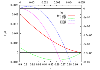
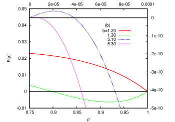
Figure 2: Function $F(\rho)$ near the phase transitions at $b_{c,1}$(with $\rho\sim 1$, left and bottom axis) and at $b_{c,2}$ (with $\rho\sim 0$, right and upper axis) for $z=4$ and two temperatures (a) $T=1$ and (b) $T=0.1$.

The zeros of $\frac{d}{d\rho}F(\rho)$ near $\rho=1$ and near $\rho=0$ give the location of the phase transitions at $b_{c,1}$ and $b_{c,2}$ , respectively. The nature of the phase transition (continuous or discontinuous) can be obtained from the sign of the second order derivative of $F(\rho)$ at the phase transition[54]. The results obtained by integrating the equations (7) until $\left|R(DD,t)\right|<10^{-12}$, for $z=2,3,4$ and $5$ are presented in Fig. 1. The behavior of $F(\rho)$ near $\rho=1$ and $\rho=0$ with density values separated by $d\rho=10^{-5}$ was used to locate the phase transitions with an error in the temptation parameter given by $db=10^{-4}$. Both phase transitions are predicted to be continuous at any temperature and for any coordination number, $z$ . In agreement with the high temperature expansion results shown in Eq. (6) we obtained values of $b_{c,1}$ almost independent of temperature and values of $b_{c,2}$ that increase for low temperatures from high temperature values close to 3. At low temperatures the values of $b_{c,2}$ are close to $z+1$. In Fig. 2 we show the behavior of $F(\rho)$ near the two phase transitions for $z=4$ and two temperatures $T=1$ (Fig. 2(a) )and $T=0.1$ (Fig. 2(b) ). Note that, at low T, the determination of the zeros of $F(\rho)$, corresponding to the transition at $b_{c,2}\sim z+1$, require a high numerical precision due to the very small value taken by $F(\rho)$ near the origin. From the lower panel of Fig. 2 it is clear that the phase with zero density of cooperators becomes stable only for high values of the temptation parameter close to $b\sim 5.2$.

4.2 $z=1$ case

The time integration of the pair mean-field equations and simulations, for $z=1$, show that the two critical temptations are equal, $b_{c,1}=b_{c,2}=3$, at any temperature, also in agreement with the high temperature expansion result Eq. (6).

$i$	Configuration	$\Delta P$
1	⋯→D→C→C→⋯	2-b
2	⋯→D→C→D→⋯	1-b
3	⋯→C→D→D→⋯	-1
4	⋯→C→D→C→⋯	b-1

Table 3: Payoff diferences, $\Delta P=P_{i_{\mu}}-P_{i}$ between strategies at $\cdots\rightarrow D\rightarrow C\rightarrow\cdots$ (configurations $1$ and $2$) and $\cdots\rightarrow C\rightarrow D\rightarrow\cdots$ (configurations $3$ and $4$) interfaces for the model with self-interaction with $z=1$.

This behavior can be understood by looking at the payoff differences, $\Delta P=P_{i_{\mu}}-P_{i}$ , listed in Table 3 for the possible configurations at the interfaces $D\rightarrow C$ (configurations $1$ and $2$ in Table 3) and $C\rightarrow D$ (configurations $3$ and $4$ in Table 3). The behavior of the system is controlled by the rates associated with the motion of the interfaces $\cdots\rightarrow D\rightarrow C\rightarrow C\rightarrow\cdots$ and $\cdots\rightarrow C\rightarrow D\rightarrow D\rightarrow\cdots$ (configurations $1$ and $3$, respectively) because the motion of the other interfaces lead to the generation of configurations of these two types. For $b\leq 1$ the rates for the displacement of $D\rightarrow C$ interfaces are higher than the rates for $C\rightarrow D$ interfaces. For $b\geq 3/2$, the rate of increase of the number of defectors associated with configuration $\cdots\rightarrow C\rightarrow D\rightarrow C\rightarrow\cdots$ (configuration $4$) becomes the higher rate in the system but it generates configurations $\cdots\rightarrow C\rightarrow D\rightarrow D\rightarrow\cdots$ ( configuration $3$) which moves, until $b=3$, at a lower rate than the rate for the spreading of cooperators $\cdots\rightarrow D\rightarrow C\rightarrow C\rightarrow\cdots$ (configuration $1$). Consequently, we expect, for $b<b_{c}=3$, the system to reach full cooperation and, for $b>b_{c}=3$, the system to reach full defection. This scenario remains valid at any nonzero temperature in spite of the temperature dependence of the rates of motion of the interfaces. This behavior is also in agreement with the results obtained for the pair approximation and simulations for $T=10$ and $T=1$ shown in Figs. 4(a) and (b), respectively. The time integration of the pair approximation equations reaches full cooperation and full defection very slowly especially at high temperatures (see the two curves shown in Fig. 4(a) obtained for a maximum integration time $10^{6}$ and $10^{7}$ where full cooperation for $b<b_{c}=3$ and full defection for $b>b_{c}=3$ are still far from being reached). In the same figure we also show the results of simulations for systems of size $N=10^{3}$ and $N=10^{4}$ showing a strong size dependence but approaching the expected behavior in the thermodynamic limit.

For the pair approximation, we have found that, exactly at $b=b_{c}=3$, $\rho(\infty)$ depends on temperature and initial condition and is given by the following expression:

$$\rho(\infty)=\frac{\left({e}^{2\,\beta}\text{\textminus}{e}^{\beta}\right)\,{\rho\left(0\right)}^{2}+\left({e}^{\beta}+1\right)\,\rho\left(0\right)}{{e}^{2\,\beta}\text{+}1-\left({e}^{3\,\beta}\text{\textminus}{e}^{2\,\beta}+{e}^{\beta}\text{\textminus}1\right)\,\rho\left(0\right)\left(\rho\left(0\right)-1\right)}.$$ (8)

Results from simulations presented in Fig. 3 agree with the pair approximation result (Eq (8)) at high temperatures and show some deviation at low temperatures.

At $T=\infty$, each agent adopts the strategy of a randomly selected neighbor with probability $\frac{1}{2}$ and the model is related to the direct voter model on directed networks considered in Ref. [53]. In this limit, the density of cooperators is conserved and it remains equal to its initial value.

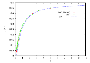
Figure 3: The stationary density of cooperators, $\rho(\infty)$ for $z=1$ and $b=3$ as a function of temperature from the pair approximation (PA, Eq. (8) ) and simulations for systems of size $N=10^{3}$and $N=10^{4}$, taking averages over $10^{4}$ samples and starting from an equal density of cooperators and defectors.

At $T=0$ the interface dynamics becomes deterministic and some of the interfaces are frozen while others are moving depending on the value of $b$ (only interfaces with $\Delta P\geq 0$ move) . For $b\leq 1$ only the $D\rightarrow C$ interfaces are active and the system should reach full cooperation (except for frozen initial domains of defectors with a negligible weight in large systems). For $b>1$ the interface $\cdots\rightarrow D\rightarrow C\rightarrow D\rightarrow\cdots$ is frozen and defectors with a neighbor cooperator that has a neighbor defector start to survive and for $b\geq 2$ the only active interface corresponds to the configuration $\cdots\rightarrow C\rightarrow D\rightarrow C\rightarrow\cdots$. After the disappearance of all cooperators with a neighbor defector that has a neighbor cooperator the system will reach a frozen disordered state, free of such configurations, with a final density of cooperators that depends on its value on the starting configuration.

4.3 $z>1$ case

For networks with a number of outgoing links, $z$, larger than one there is a region of coexistence of strategies for $b$ values between the two critical parameters $b_{c,1}$ and $b_{c,2}$. In Fig. 4 we show, for $z=2,\,4$ and $10$ the stationary density of cooperators obtained by simulations of systems of size $N=10^{4}$ for $T=10$ (Fig. 4(a) ) and $T=1$ (Fig. 4(b) ) taking averages over $100$ samples. In all our simulations the stationary averages were obtained by neglecting the initial transient time dependence and averaging only over samples that have not reached any of the two absorbing states (full cooperation and full defection). We also plot the pair approximation predictions showing a good agreement with MC simulations except near the phase transitions where slightly different values for the critical temptation parameters are obtained. In the pair approximation, for the network with $z=4$ at $T=1$ we got $b_{c,1}=1.2542(1)$ and $b_{c,2}=3.3241(1)$ and results from simulations give $b_{c,1}=1.274(1)$ and $b_{c,2}=3.14(1)$. Furthermore, the agreement between simulations and the pair approximation worsens as the temperature decreases.

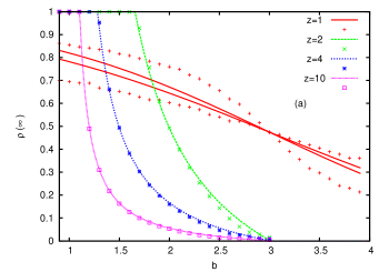
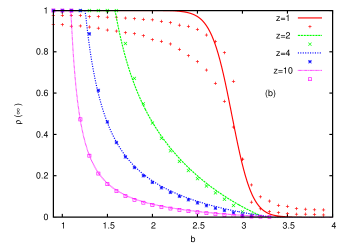
Figure 4: Comparison of the predictions of the pair approximation (lines) and Monte Carlo simulations (points) for the stationary density of cooperators $\rho(\infty)$ for (a) $T=10$ and (b) $T=1$. The simulations were done for systems of size $N=10^{4}$ and averages were made over $100$ samples. For $z=1$ simulations are shown for system sizes $N=10^{3}$and $10^{4}$ taking averages over $10^{4}$ samples. For the pair approximation the $z=1$ results are not stationary and correspond to cooperator densities reached at integration times $10^{6}$ and $10^{7}$in (a) and $10^{6}$in (b).

The payoff differences at $D\rightarrow C$ interfaces take the possible values $\Delta P_{D\rightarrow C}=m+1-n\,b$ with $0\leq m\leq z$ and $1\leq n\leq z$ and at $C\rightarrow D$ interfaces take the values $\Delta P_{C\rightarrow D}=n\,b-m-1$ with $0\leq m\leq z-1$ and $0\leq n\leq z$, where $m$ and $n$ are the possible number of cooperators in the neighborhood of the cooperator and of the defector, respectively. At low temperatures, the dynamics at interfaces with negative payoff differences is slow ( freezing at $T=0$) which generates plateaus in the density of cooperators in between the values of temptation, $b_{n,m}=\frac{m+1}{n}$, where the payoffs for the interfaces change sign.

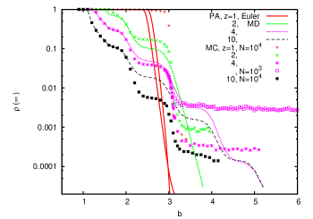
Figure 5: We compare the temptation dependence of the stationary density of cooperators, $\rho(\infty)$ , for pair approximation (PA) and Monte Carlo simulations (MC) at a low temperature, $T=0.1$, for networks with $z=1,\>2,\>4$ and $10$. The PA results for $z=1$ were obtained from time integration for $10^{6}$and $10^{7}$ steps showing a slow approach to the stationary behavior. Results for other values of $z$ were obtained from Eq. 7(MD) . The MC results were obtained for systems of size $N=10^{4}$ and $N=10^{3}$ (for $z=4$) to show the finite size effects at large values of $b$, for very small densities of cooperators.

Near the full cooperator state the most important configurations for the $D\rightarrow C$ interfaces correspond to $m=z$ and $n=z$ which becomes inactive ( stopping creating cooperators), at very low T, for $b>b_{z,z}=1+1/z$ meaning that an isolated $D$ in a sea of $C$ start surviving. The most important configuration for the $C\rightarrow D$ interface, near the full cooperator state, correspond to $m=z-1$ and $n=z$ which becomes active (starting creating defectors), at very low T, for $b>b_{z,z-1}=1$. These defectors will be at new $C\rightarrow D$ interfaces where the defector now has a neighboring defector and the new interface is active and leading to the creation of new defectors for $b>b_{z-1,z-1}=1/(1-1/z)\sim 1+1/z$ . This explains the observation of values of $b_{c,1}$ close to 1, in agreement with the high temperature expansion, Eq. (6), which gives a dependence on the network coordination number approaching 1 in the limit of an infinite number of neighbors.

The most important configurations for $D\rightarrow C$ interfaces, near the full defection state, correspond to $m=0$ and $n=1$ with $\Delta P_{D\rightarrow C}=1-b$ and for the $C\rightarrow D$ interface $m=0$ and $n=0$ with $\Delta P_{C\rightarrow D}=-1$ . However the motion of the $D\rightarrow C$ interface with $m=0$ and $n=1$ generates a new cooperator which will be at a $D\rightarrow C$ interface with $m=1$ and $n=1$ corresponding to $\Delta P_{D\rightarrow C}=2-b$ . Thus, like in the case for $z=1$, we would expect that the processes that generate defectors will win over those that generate cooperators for $b>b_{c,2}\sim 3$ . At very low T, since cooperators without any neighboring cooperators always have higher payoffs than defectors also without neighboring cooperators, independently of $b$, the interfaces $C\rightarrow D$ will be sluggish, and cooperators may persist in the system for long times. Furthermore, clusters of cooperators with a $C$ connected to other $C$ resist as long as the weakest cooperators, in the periphery of the cluster, with no neighboring cooperators resist invasion by defectors. The $C$ in the root of a cluster connected to $z$ cooperators is a source of new $C$ up to $b=z+1$. The newly generated cooperators, in the new roots, have only one neighboring $C$ and, for values of $b>2$, do not generate further spreading of cooperators. At a finite, low $T$, the balance between the rate of disappearance of $C$ in the periphery of the cluster, where the cooperators have no neighboring cooperators, and the rate of creation of new $C$, from a $C$ with only one neighboring $C$ remains the most important balance leading to $b_{c,2}=3.$ However, the pair approximation is not sensitive to the weakness of the newly generated cooperators and shows incorrectly, at low temperatures, $b_{c,2}\sim z+1$, which is the temptation limit above which, at zero temperature, all the processes generating cooperators stop.

In Fig. 5 we show for the low temperature, $T=0.1$, the stationary density of cooperators, $\rho(\infty)$, as a function of $b$, obtained from simulations and the pair approximation for systems of $z=2,\,4$ and $10$. The pair approximation results were obtained from the modified dynamics (MD) Eq. (7) and time integration of the mean-field equations (Eq. (4)) (for $z=1$). The agreement of the pair approximation with simulations is good for small values of $b$, but the height of the plateaus in $\rho(\infty)$, for $b\geq 2$, when $\rho(\infty)\lesssim 0.1$, are not correctly predicted by the pair approximation. The simulation results for $z=4$ and sizes $N=10^{3}$ and $10^{4}$ show that for $b\gtrsim 3$ the observed plateaus have heights that decrease with the size of the system suggesting that in the thermodynamic limit the system reaches the full defection absorbing state. We determined $b_{c,2}$ from simulations of the time dependent behavior of $\rho(t)$ for a network with $z=4$ and size $N=10^{6}$ (see Fig. 6) obtaining $b_{c,2}=3.11(1)$ which is much smaller than the value $b_{c,2}\sim 5$ predicted by the pair approximation. For large times we observe $\rho(t)\sim 1/t$ as expected for the mean-field universality class of phase transitions to a single absorbing state[55].

It is interesting to comment on the behavior of the system for increasing values of $z$: for very large $z$, we approach the fully connected network limit, where it is known that the system jumps from full cooperation to full defection at $b=1$. Our results show that for large $z$, the critical temptation $b_{c,1}$ gets closer to $1$ and the density of cooperators decays very strongly for $b>b_{c.1}$ but still shows a small nonzero value for temptation values up to $b_{c,2}$ which does not approach $b_{c,1}$ for arbitrary large $z$.

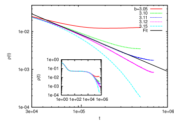
Figure 6: Monte Carlo simulations of the time dependence of the density of cooperators, $\rho(t)$, at a low temperature $T=0.1$ for a network with $z=4$ with a system size $N=10^{6}$ showing that $b_{c,2}=3.11(1)$, much smaller than the value predicted by the pair approximation. The power law fit of $\rho(t)$, for large times, shown in the plot, has a slope $\alpha=-0.998$. In the inset we present the full curve $\rho(t)$ including the behavior at short times.

4.4 model without self-interaction

We can repeat the above arguments for the model without self-interaction and conclude that for $z=1$ we have, $b_{c,1}=b_{c,2}=1$ with a suppression of cooperation for $b>1$ . For larger $z$ we have now $b_{n,m}=\frac{m}{n}$ and near the full cooperator state a single $D$ at a $D\rightarrow C$ interface start surviving, at low $T$, for $b>b_{z,z}=1$. The $C\rightarrow D$ interfaces with $m=z-1$ and $n=z$ lead to new $C\rightarrow D$ interfaces with $m=z-1$ and $n=z-1$ which are active and leading to the proliferation of defectors, for $b>b_{z-1,z-1}=1$. Consequently, we expect $b_{c,1}\sim 1$. Considering now configurations close to the full defection state we see that a single cooperator at a $C\rightarrow D$ interface in a sea of defectors has $\triangle P_{C\rightarrow D}=0$ and such interface is always active. The $D\rightarrow C$ interface for the cooperator in the sea of defectors $(m=0$ and $n=1$ ) has $\triangle P_{D\rightarrow C}=-b$ and it is inactive at very low $T$. The production of $C$ occurs predominantly at configurations where a $C$ has a neighboring $C$ $(m=1$ and $n=1$ ) with $\triangle P_{D\rightarrow C}=1-b$ and the balance between $C$ production and $D$ production turns in favor of defectors for $b>b_{c,2}\sim 1$. From an high temperature expansion (weak selection limit) we obtained from the pair approximation:

$$\begin{array}[]{cl}b_{c,1}&=1-\frac{1}{T}\,\frac{\left(z-1\right)^{2}}{8z^{3}-12z^{2}+6z-1}\\ b_{c,2}&=1+\frac{1}{T}\,\frac{\left(z-1\right)^{2}}{\left(2z-1\right)^{2}}\end{array}.$$ (9)

Contrary to the case with self-interaction a cluster of $C$ in a sea of $D$ is not stable at low T because now the cooperators in the periphery (with no neighboring $C$) do not resist invasion by defectors. Consider the cluster $D\rightarrow C\rightarrow C\rightarrow D$ with a $D\rightarrow C$ and a $C\rightarrow D$ interface and consider that the remaining neighbors are all $D$ . At $T=0$, the $D\rightarrow C$ interface is frozen for $b>1$ and the activity at the interface $C\rightarrow D$ leads to the disappearance of the cooperators. For the cluster to be sustainable there is need for the interfaces $C\rightarrow D$ in the periphery to move at a lower rate than the interfaces $D\rightarrow C$ at the root which leads to the balance being in favor of defectors for $b>1$. When the defector at the $D\rightarrow C$ interface is facing a $C$ with, for example, two neighboring $C,$ then cooperators are generated with higher rate determined by the payoff difference $2-b$ but still the newly generated $C$ will have only one $C$ neighbor and again for $b>1$ defectors will win. In Fig.7 we show the pair approximation phase diagram using the same method previously applied to the model with self-interaction. In the inset we see that the high temperature expansion Eq. 9 agrees well with the numerical results.

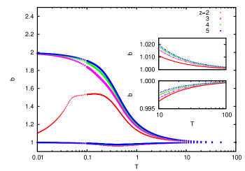
Figure 7: Phase diagram of the model without self-interaction, in the pair approximation, for the out-homogeneous networks with $z=2,3,4$ and $5$. The lower curves are $b_{c,1}$ and the upper curves are $b_{c,2}$, respectively. The inset shows the high temperature region where the numerical results based on Eq. (7) are compared with the analytical results (lines) presented in Eq. (9).

At very low $T$ we obtain for the pair approximation a value $b_{c,2}\sim 1$ for $z=2$ and $b_{c,2}\sim 2$ for $z>2$. This difference in behavior may be related with the different relative statistical weight given by the pair approximation to configurations with a $C$ with one and two $C$ as neighbors for $z=2$ and $z>2$ because if the configurations with two neighboring $C$ are predominant we expect the rate of creation of $C$ to be determined by the payoff difference $2-b$ leading to $b_{c,2}\sim 2$ . We made MC simulations of networks with, $z=2,4$ and $10$, at a low temperature, $T=0.1$ , and the results shown in Fig. 8 correspond to a value $b_{c,2}\sim 1.2$ much smaller than the pair approximation prediction.

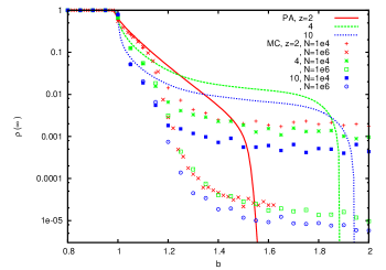
Figure 8: Comparison of pair approximation (PA) and MC simulation results for the steady state density of cooperators for the model without self-interaction at a low temperature $T=0.1$ and for out-homogeneous directed networks with $z=2$, $4$ and $10$.

5 Random directed networks

In random directed networks the distribution of the number of outgoing links of a given vertex is Poissonian and strongly peaked at its average number. The behavior of the stationary density of cooperators is expected to follow the same trend as for out-homogeneous directed random networks with a given number of outgoing links. To test the accuracy of the mean-field pair approximation in Eq. (4) for an heterogeneous case we compared it with MC simulations, for the model with self-interaction at $T=1$ for different average number of out-neighbors. The results in Fig. 9 show that the pair approximation provides a reasonably good approximation for the behavior of the system. Since we use a modified Poissonian distribution, as described in section 2, the limit $q\rightarrow 0$ of these networks corresponds exactly to out-homogeneous networks with $z=1$.

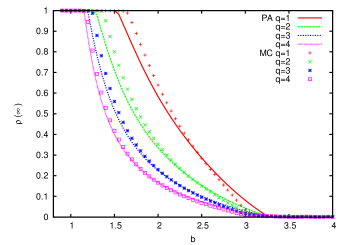
Figure 9: Comparison of the pair approximation (PA) and simulations (MC) of the PD model with self-interaction for uncorrelated directed random networks with size $N=10^{4}$, with average number of neighbors, $\left\langle z\right\rangle=1.582$ (q=1), $2.313$ (q=2), $\left\langle z\right\rangle=3.1572$ (q=3) and $\left\langle z\right\rangle=4.0746$ (q=4).

6 Concluding Remarks

We have derived an heterogeneous pair mean-field approximation that is able to correctly describe the behavior of the prisoner’s dilemma model in directed networks in the limit of high T (weak selection). At low T the pair approximation gives predictions for the critical parameter $b_{c,2}$ in disagreement with MC simulation. The pair approximation was numerically studied by using a very efficient method, previously applied to other models[54], which is based on modified dynamical equations that solve the time-dependent equations under the constraint of a given density of cooperators. We also obtained analytical expressions for the two critical parameters $b_{c,1}$ and $b_{c,2}$ in the limit of high temperature. For the model with self-interaction $b_{c,1}$ has a weak temperature dependence and approaches $1$ for large $z$ and $b_{c,2}$ is close but larger than $3$ for any $z$. Without self-interaction, at any temperature, $b_{c,1}$ is close but smaller than $1$ and $b_{c,2}$ is greater but close to 1 . Essentially, the inclusion of the self-interaction promotes a shift of $b_{c,2}$ from values close to $1$ to values close to $3$. The case $z=1$ is a special case where, in both cases, $b_{c,1}=b_{c,2}$, independent of temperature. In the model without self-interaction we find $b_{c,1}=b_{c,2}=1$ and cooperation is fully suppressed for $b>1$ while in the model with self-interaction the full cooperator state is still reached for temptation values up to $b_{c,1}=b_{c,2}=3$. In both models the coexistence region does not shrink as $z$ increases but the levels of cooperation strongly decrease with increasing $z$, as the networks get closer to the fully connected limit. This behavior is similar to the one previously reported for one-dimensional regular lattices with varying coordination number[22]. We can also compare our results to other available results for non-directed lattices and random networks. The inclusion of self-interaction increases $b_{c,2}$ from $\sim 1.035$ to $\sim 1.85$, at $T=0.1$ in the square lattice (see Refs [13, 14]) while in our out-homogeneous directed networks we observe a much larger increase in $b_{c,2}$. In previous studies of non-directed lattices and random regular graphs[14, 24] two types of phase diagrams were found: (1) one where $b_{c,2}$ shows a non-monotonous dependence with $T$ , being equal to $1$ at $T=0$ and $T=\infty$ and (2) another type where $b_{c,2}$ decreases with $T$ showing the highest value in the noise-free limit $T=0$ . Our MC simulation results suggest that the phase diagram in the directed networks studied here are of the first type showing an equal high and low $T$ limits for $b_{c,2}$ although not equal to $1$ in the case of the model with self-interaction. It is not clear if it is possible to observe phase diagrams of type (2) in directed networks. Our main results were obtained for out-homogeneous networks but we expect the main conclusions to apply also to directed random networks with Poissonian in and out degree distributions.

The study of evolutionary dynamics in other types of directed networks and in mixed directed/ non-directed networks taking into consideration the difference between interaction and learning/reproduction networks may be relevant for the modeling of real systems.

References

- [1] Kollock P 1998 Annu. Rev. Sociol. 24 183–214
- [2] Nowak M A 2006 Evolutionary dynamics: exploring the equations of life. (Harvard University Press, Cambridge, Massachussets)
- [3] Szabó G and Fáth G 2007 Physics Reports 446 97
- [4] Sigmund K 2010 The Calculus of Selfishness (Princeton University Press, New Jersey)
- [5] Axelrod R and Hamilton W D 1981 Science 211 1390–1396
- [6] Axelrod R 1984 The Evolution of Cooperation (Basic Books, New York)
- [7] Nowak M A 2006 Science 314 1560–63
- [8] Nowak M A and May R M 1992 Nature 359 826–29
- [9] Nowak M A and May R M 1993 Int. J. Bif. and Chaos 3 35
- [10] Nowak M A, Bonhoeffer S and May R M 1994 Int. J. Bif. and Chaos 4 33–56
- [11] Lindgren K and Nordahl M 1994 Physica D 75 292
- [12] Hauert C and Szabó G 2005 Am. J. Phys 73 405
- [13] Szabó G and Töke C 1998 Phys. Rev. E 58 69
- [14] Szabó G, Vukov J and Szolnoki A 2005 Phys. Rev. E 72 047107
- [15] Vukov J and Szabó G 2005 Phys. Rev. E 71 036133
- [16] Holme P, Trusina A, Kim B J and Minnhagen P 2003 Phys. Rev. E 68 030901R
- [17] Abramson G and Kuperman M 2002 Phys, Rev. E 63 030901R
- [18] Kim B J, Trusina A, Holme P, Minnhagen P, Chung J S and Choi M Y 2002 Phys. Rev. E 66 021907
- [19] Masuda N and Aihara K 2003 Physics Letters A 313 55–61
- [20] Tomochi M 2004 Social Networks 309 26
- [21] Santos F C, Rodrigues J F and Pacheco J M 2005 Phys. Rev. E 72 056128
- [22] Pacheco J M and Santos F C 2005 in Science of Complex Networks: From Biology to the Internet and WWW. (Mendes, J.F.F. (Ed.), AIP Conf. Proc. No. 776. AIP, Melville, NY, pp. 90-100)
- [23] Tang C L, Wang W X, Wu X and Wang B H 2006 Eur. Phys. J. B 53 411–15
- [24] Vukov J, Szabó G and Szolnoki A 2006 Phys. Rev. E 73 067103
- [25] Santos F C, Pacheco J M and Lenaerts T 2006 Proc. Nat. Acad. Sciences 103 3490–4
- [26] Santos F C and Pacheco J M 2005 Phys. Rev. Lett. 95 098104
- [27] Santos F C, Rodrigues J F and Pacheco J M 2006 Proc. R. Soc. B 273 51–55
- [28] Ohtsuki H, Hauert C, Lieberman E and Nowak M A 2006 Nature 502 441
- [29] Maciejewski W, Fu F and Hauert C 2014 PLoS Comput Biol 10 e1003567
- [30] Ohtsuki H, Nowak M A and Pacheco J M 2007 Phys. Rev. Lett 98 108106
- [31] Ohtsuki H, Pacheco J M and Nowak M A 2007 Journal of Theoretical Biology 246 681–94
- [32] Wu Z X and Wang Y H 2007 Phys. Rev. E 75 041114
- [33] Guha R, Kumar R, Raghavan P and Tomkins A 2004 Propagation of trust and distrust Proceedings of the 13th International Conference on World Wide Web WWW ’04 (New York, NY, USA: ACM) pp 403–412
- [34] Wu Z X, Xu X J, Huang Z G, Wang S J and Wang Y H 2006 Phys. Rev. E 74 021107
- [35] Skyrms B and Pemantle R 2000 Proc. Natl. Acad. Sci. USA 97 9340–46
- [36] Lipowski A, Lipowska D and Ferreira A L 2014 Phys. Rev. E 90 032817
- [37] Lieberman E, Hauert C and Nowak M A 2005 Nature 433 312
- [38] Ohtsuki H and Nowak M A 2006 Proc. R. Soc. B 273 2249
- [39] Ohtsuki H and Nowak M A 2008 Journal of Theoretical Biology 251 698–707
- [40] Ferreira A L and Mendiratta S K 1993 J. Phys A: Math. Gen. 26 L145
- [41] ben Avraham D and Köhler J 1992 Phys, Rev. A 45 8358
- [42] Petermann T and Rios P D L 2004 Journal of Theoretical Biology 229 1–11
- [43] Lipowski A, Ferreira A L, Lipowska D and Gontarek K 2015 Phys. Rev. E 92 052811
- [44] Dorogovtsev S N, Goltsev A V and Mendes J F F 2008 Rev. Mod. Phys 80 1275
- [45] Vespignani A 2012 Nature Physics 8 32
- [46] Pastor-Satorras R and Vespignani A 2001 Phys. Rev. Lett. 86 3200
- [47] Mata A S, Ferreira R S and Ferreira S C 2014 New J. Phys. 16 053006
- [48] Ohtsuki H, and Nowak M A 2006 Journal of Theoretical Biology 243 86–97
- [49] Lipowski A, Gontarek K and Lipowska D 2014 Phys. Rev. E 91 062801
- [50] Molloy M and Reed B 1995 Random Struct. Algorithms 6 161
- [51] Dorogovtsev S N, Mendes J F F and Samukhin A N 2001 Phys. Rev. E 64 025101(R)
- [52] Boguná M and Serrano M A 2005 Phys. Rev. E 72 016106
- [53] Serrano M A, Klemm K, Vazquez F, Eguíluz V M and Miguel M S 2009 Journal of Statistical Mechanics: Theory and Experiment 2009 P10024 URL http://stacks.iop.org/1742-5468/2009/i=10/a=P10024
- [54] Pedro T B, Figueiredo W and Ferreira A L 2015 Phys. Rev. E 92 032131
- [55] Marro J and Dickman R 1999 Nonequilibrium Phase Transitions in Lattice Models (Cambridge, U.K: Cambridge University Press)