Cell-veto Monte Carlo algorithm for long-range systems
Abstract
We present a rigorous efficient event-chain Monte Carlo algorithm for long-range interacting particle systems. Using a cell-veto scheme within the factorized Metropolis algorithm, we compute each single-particle move with a fixed number of operations. For slowly decaying potentials such as Coulomb interactions, screening line charges allow us to take into account periodic boundary conditions. We discuss the performance of the cell-veto Monte Carlo algorithm for general inverse-power-law potentials, and illustrate how it provides a new outlook on one of the prominent bottlenecks in large-scale atomistic Monte Carlo simulations.
Markov-chain Monte Carlo is one of the most widely used computational methods in the natural sciences. It samples a high-dimensional space of configurations according to a probability distribution . In the physical sciences, generally corresponds to the Boltzmann distribution , where is the inverse temperature and the system energy. The core of most Monte Carlo computations is the Metropolis algorithm Metropolis et al. (1953), which accepts a trial move from configuration to configuration with probability
| (1) |
The acceptance probability Eq. 1 satisfies the detailed balance condition, , that leads to exponential convergence towards the stationary distribution , if ergodicity is assured Krauth (2006). Moving from one configuration to another requires evaluating the induced change of the system energy. In most classical -particle simulations, the system energy is a sum over pair terms: with the pair potential and the interparticle distances . The evaluation of the system energy generally takes operations, and the computation of the energy change upon moving a single particle takes operations. For a potential with finite support, the change of the system energy for moving one particle is computed in . To speed up the evaluation, potentials with infinite support, such as the Lennard-Jones and other moderately long-ranged potentials, are truncated beyond an effective interaction range. This approximation is however known to alter the equilibrium properties Smit (1992); in ’t Veld et al. (2007). Strongly long-ranged potentials, as they appear in electrostatics and gravity, do not allow for the definition of a finite interaction range and require specialized techniques for determining the system energy to high precision. Ewald summation de Leeuw et al. (1980); Frenkel and Smit (2001), for example, adds and subtracts smooth charge distributions localized around the point particles. With periodic boundary conditions, this turns the long-ranged part of the interaction into a rapidly converging sum in Fourier space. Ewald summation computes the system energy in , taking into account periodically replicated images of the particles Perram et al. (1988); Frenkel and Smit (2001). Its refinements further reduce the burden of the system-energy computation by discretizing the charge density Eastwood and Hockney (1974) or by exploiting large-scale uniformity Greengard and Rokhlin (1987). Still, in many outstanding applications in the natural sciences, the evaluation of long-ranged potentials remains a computational bottleneck. Implementing Ewald summation is particularly difficult if periodic boundary conditions are not realized in all dimensions, as for example in slab geometries Bródka (2004); Mazars (2011).
In this paper, we present a rigorous Monte Carlo algorithm for particle systems with long-ranged interactions that does not evaluate the system energy, in contrast to virtually all existing Markov-chain Monte Carlo algorithms Krauth (2006). This change of perspective opens up many opportunities: Based on a cell-veto scheme within the factorized Metropolis algorithm Michel et al. (2014), it implements a single-particle move in complexity without any truncation error. For moderately long-ranged potentials, such as Lennard-Jones or dipolar interactions, the step size is independent of the system size, and the algorithm is effectively constant-time. For strongly long-ranged interactions, as the Coulomb forces, the single-move step size slightly decreases with . For concreteness, we will consider a fixed hypercubic box of size with periodic boundary conditions, where is the dimension of physical space. The generalization to slab geometries is straightforward.
In contrast to the Metropolis algorithm of Eq. 1, the pairwise factorized algorithmMichel et al. (2014) accepts moves with the probability
| (2) |
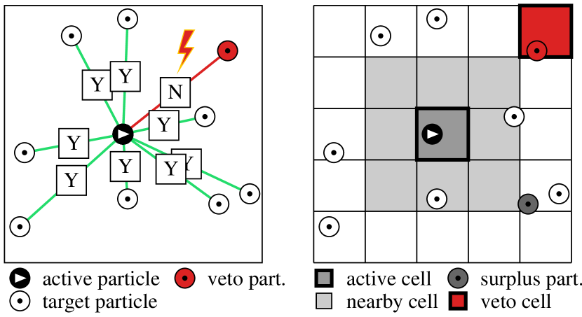
where is the change in the pair potential between particles and . In our algorithm, we never explicitly evaluate the function . Rather, the product of probabilities on the rhs of Eq. (2) is interpreted as a condition that is true if all its factors are true. The move is thus accepted by consensus, namely if each pair independently accepts the move with probability Michel et al. (2014) (see Fig. 1). Instead of computing the energy to high precision, we will compute upper bounds for the veto probability by embedding particles and into cells and , respectively. To identify particles vetoing the move, one rapidly identifies cell vetos and inspects the contents of corresponding cells to determine whether the cell vetos are confirmed on the particle level (see Fig. 1).
In continuum space, two configurations and with can be infinitesimally close to each other. For regular potentials, this implies that the change of pair energies , and therefore the veto probability , are infinitesimal as well. In the event-chain algorithm Bernard et al. (2009); Michel et al. (2014), a proposed move consists in the infinitesimal displacement of an “active” particle in a direction : The proposed move is , where is an infinitesimal time increment. The active particle keeps moving in the same direction until a move is finally vetoed by a target particle . The target particle then becomes the new active particle, i. e., the proposed move is , and if vetoed by particle pair , the configuration is changed to . This implements a “lifted” Markov chain Diaconis et al. (2000) with two additional variables and , which trivially projects to the physical space with the proper Boltzmann distribution. Veto probabilities are infinitesimal. Two simultaneous vetos are thus prevented from arising from different target particles. Detailed balance is violated (the reverse move is never proposed). However, the event-chain algorithm satisfies the global-balance condition
| (3) |
sufficient for exponential convergence to the equilibrium distribution on the accessible configurations. To ensure ergodicity, both the active particle and the direction of motion are periodically reset to random values (see Supp. 2). Lifted Markov chains have been shown to improve convergence speed in many cases, and also to lower the dynamical critical scaling exponents Diaconis et al. (2000); Kapfer and Krauth (2015); Michel et al. (2015); Nishikawa et al. (2015).
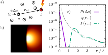
The core of an event-chain program consists in determining the step size to the next particle event and in identifying the vetoing target particle , rather than explicitly programming small time increments (see Fig. 2a). The actual move then merely consists in updating the active particle position as and in changing the active particle to . For long-ranged potentials, can be far away from the active particle. At any instant during the simulation, the veto probability of a potential target particle is given by the particle-event rate , defined via a directional derivative of the pair potential,
| (4) |
with . For long-ranged potentials, carries over large distances (see Fig. 2b, c). Particle-event distances are distributed as , where is the radial distribution function, and thus exhibit the same long-ranged tail. In contrast, the displacement between events, i. e., the step size , decays exponentially within a few interparticle distances, see Fig. 2c. For each pair , the event time can be computed in , so that the event-chain algorithm can be implemented in per particle event Peters and de With (2012), by iterating over all target particles. The earliest veto will define the step size and the active particle for the next step.
For a homogeneous system (with a bounded particle density), the complexity per particle event can be reduced from to by establishing upper bounds for the particle-event rate which hold irrespective of the precise particle positions. Concretely, we superimpose a fixed regular grid onto the system, with cells typically containing at most one particle (see Fig. 1; rare “surplus” particles are treated separately). The particle-event rate between the active particle in cell and a target particle in cell is bounded from above by the cell-veto rate
| (5) |
This quantity depends only on the pair potential and the relative positions of the two cells and can be tabulated before sampling starts. The cell-veto rate remains finite except for a few nearby cells that contain the hard-core singularities. In the case of point particles, these must include any cells that share corners with (see Fig. 1). For efficiency, “nearby” cells may comprise a larger portion of the short-range features of .
Excluding nearby and surplus particles, the total particle-event rate is bounded from above by the total cell-veto rate
| (6) |
which remains a constant throughout the simulation. The next cell veto can then be sampled in : The time is distributed exponentially
| (7) |
so that is given through the logarithm of a uniform random number (Krauth (2006), see Supp. 2). The cell veto is triggered by the cell with probability . The selection of the target cell from all the non-nearby cells can also be accomplished in constant time (see below). If the vetoing cell contains a particle, at position , it is then chosen as the target particle for a particle event with probability . This long-range particle event must be put into competition with events triggered by nearby or surplus particles, which are handled as in the short-range event-chain algorithm Michel et al. (2014) (see also Supp. 2). The number of nearby particles is naturally bounded. The number of surplus particles may be kept as small as desired by adapting the cell size. In practice, we use cells that are sufficiently small so that surplus particles appear only exceptionally. Consequently, a cell veto can effectively be processed constant time, and the performance of the cell-veto algorithm depends on the rate of cell vetos .
The total cell-veto rate depends on the range of the pair potential. For inverse-power-law interactions, , the event rate for a bare particle scales as 111We set, for , and for , , i. e., planar Coulomb; here and are the scales of energy and length. In either case, . . In an infinite system, the total cell-veto rate is finite for moderately long-ranged potentials, i. e., for . This class includes dipolar forces in and , as well as the Lennard-Jones potential. In this case, the cell-veto algorithm is of complexity .

For strongly long-ranged potentials (, including Coulomb forces), the cell-veto rate in an infinite system diverges (see Fig. 3a). In the replicated-box representation of periodic boundary conditions (see Fig. 4), even the sum over all periodic images of a single target particle () leads to an infinite particle-event rate. The sum may be regularized by adding uniformly charged line segments (parallel to the direction of motion ) that neutralize each particle charge yet combined leave invariant the energy differences of the original system. Screening line charges can be defined for general potentials. For inverse-power-law interactions, the directional derivatives of the particle and line-charge potentials are
| (8) | ||||
| (9) |
where is the folded-out distance vector between the active particle and a particular periodic image of the target particle. By vanishing monopole and dipole moments, asymptotically decays as , sufficient to render unconditionally convergent for Coulomb forces.
We may now define three distinct particle-event rates:
| bare, | (10) | ||||
| screened, | (11) | ||||
| screened lattice. | (12) |
The screened-lattice version of Eq. (12), where the sum extends over all periodic images of the target particle, minimizes the cell-veto rate by merging the periodic images into the primary copy of each particle. The number of target cells is finite, and the target cell of a cell veto can be found extremely efficiently by precomputing the function and employing Walker’s alias method or related techniques Walker (1977); Marsaglia et al. (2004) (see Supp. 1). A commented Python implementation of the cell-veto Monte Carlo algorithm using this approach is provided in Supp. 2.
In an alternative version of the cell-veto algorithm, the particle-event rates of Eq. (10) and Eq. (11) are used with explicitly replicated simulation boxes. An infinite number of target cells are considered. The target cell for a cell veto can still be found in constant time by rejection sampling. A vector is sampled with probability density , where is an upper bound to the particle-event rate for all vectors shorter than the cell diagonal. The target cell is then the cell containing the point (see Supp. 1). The cell-veto rates are somewhat larger than for the lattice-screened version. This may however be offset by the less onerous evaluation of Eq. (10) or Eq. (11) compared to Eq. (12) (surplus particles must be treated with the lattice-screened version).
Both the screened and the screened-lattice particle-event rates overcome the divergence at with periodic boundary conditions (see Fig. 3a). Since one cell veto can be handled in operations, the computational cost of simulating a fixed timespan is proportional to the rate of cell vetos. For a distance vector , the directional derivatives in Eqs (8) and (9) scale as and so do the particle-event rates . This implies that, above the point , the cell-veto rate at constant density scales as = . For Coulomb forces in dimensions, , we find , see Fig. 3b. Thus, in three dimensions, the cell-veto algorithm is of complexity . This compares favorably with the cost of an energy evaluation with Ewald summation in conventional Metropolis Monte Carlo.

In conclusion, we have presented a cell-veto Monte Carlo algorithm that need not compute the system energy. Remarkably, it advances the physical state of the system by one event in even for long-ranged interactions. The algorithm introduces none of the cutoffs that come with practical versions of Ewald summation. Strongly long-ranged potentials such as electrostatic forces are handled exactly using screening line charges. The complexity of the algorithm then scales weakly with . It is hoped that the algorithm will permit to access much larger systems than was previously possible. The demo program of Supp. 2, and the C++ version of this algorithm are available online Pos .
References
- Metropolis et al. (1953) N. Metropolis, A. W. Rosenbluth, M. N. Rosenbluth, A. H. Teller, and E. Teller, J. Chem. Phys. 21, 1087 (1953).
- Krauth (2006) W. Krauth, Statistical Mechanics: Algorithms and Computations, Oxford Master Series in Physics (Oxford University Press, UK, 2006).
- Smit (1992) B. Smit, J. Chem. Phys. 96, 8639 (1992).
- in ’t Veld et al. (2007) P. J. in ’t Veld, A. E. Ismail, and G. S. Grest, J. Chem. Phys. 127, 144711 (2007).
- de Leeuw et al. (1980) S. W. de Leeuw, J. W. Perram, and E. R. Smith, Proc. R. Soc. A 373, 27 (1980).
- Frenkel and Smit (2001) D. Frenkel and B. Smit, Understanding Molecular Simulation: From Algorithms to Applications, Computational science series (Elsevier Science, 2001).
- Perram et al. (1988) J. W. Perram, H. G. Petersen, and S. W. de Leeuw, Mol. Phys. 65, 875 (1988).
- Eastwood and Hockney (1974) J. W. Eastwood and R. W. Hockney, J. Comput. Phys. 16, 342 (1974).
- Greengard and Rokhlin (1987) L. Greengard and V. Rokhlin, J. Comput. Phys. 73, 325 (1987).
- Bródka (2004) A. Bródka, Chemical Physics Letters 400, 62 (2004).
- Mazars (2011) M. Mazars, Physics Reports 500, 43 (2011).
- Michel et al. (2014) M. Michel, S. C. Kapfer, and W. Krauth, J. Chem. Phys. 140, 054116 (2014).
- Bernard et al. (2009) E. P. Bernard, W. Krauth, and D. B. Wilson, Phys. Rev. E 80, 056704 (2009).
- Diaconis et al. (2000) P. Diaconis, S. Holmes, and R. M. Neal, Annals of Applied Probability 10, 726 (2000).
- Kapfer and Krauth (2015) S. C. Kapfer and W. Krauth, Phys. Rev. Lett. 114, 035702 (2015).
- Michel et al. (2015) M. Michel, J. Mayer, and W. Krauth, EPL (Europhysics Letters) 112, 20003 (2015).
- Nishikawa et al. (2015) Y. Nishikawa, M. Michel, W. Krauth, and K. Hukushima, Phys. Rev. E 92, 063306 (2015).
- Peters and de With (2012) E. A. J. F. Peters and G. de With, Phys. Rev. E 85, 026703 (2012).
- Note (1) We set, for , and for , , i. e., planar Coulomb; here and are the scales of energy and length. In either case, .
- Walker (1977) A. J. Walker, ACM Trans. Math. Softw. 3, 253 (1977).
- Marsaglia et al. (2004) G. Marsaglia, W. W. Tsang, and J. Wang, Journal of Statistical Software 11, 1 (2004).
- (22) https://github.com/Cell-veto .
Supplement to “Cell-veto Monte Carlo algorithm for long-range systems”
.1 Supplementary Item 1: Cell-veto sampling
The pairwise factorized Metropolis algorithm determines pair events (vetos) and
thus avoids to compute the system energy. The cell-veto algorithm takes this
strategy one step farther. Instead of scanning all particle pairs for vetos, it
first solicits cell vetos (see Fig. 1), which then have to be
confirmed on the level of the actual particle positions. Even with periodic boundary
conditions, the number of cells remains finite if all the periodic images of a
particle are merged into the one located in the primary simulation box (see
Eq. (12)). The next cell veto must be selected from the
cells with a nonzero cell-veto rate. Each cell must be sampled
with probability , see Fig. S1.
This finite discrete-probability sampling problem is best solved through a
rejection-free exact algorithm, as Walker’s alias method. In Walker’s method,
the cell-veto rates are reassembled into composite rates consisting of at most
two original rates and adding up to exactly the mean cell-veto rate
. The cutting-up and reassembling of the constitutes the initialization stage
of Walker’s method (in the demo program of Supp. 2:
in function WalkerSet). In the sampling stage, a cell can be sampled
with the proper probability by first sampling the composite rate (as a random integer between
and ) and then deciding between
the at most two rates by sampling a uniform random real between and
(WalkerSample, in the demo program of Supp. 2).
This step is constant time and independent of the number of cells.
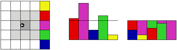
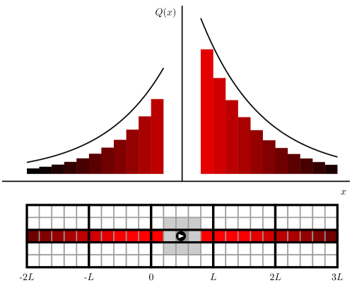
Alternatively, one may also keep the individual cells, that is, work explicitly in the folded-out version of the system, and with the cell-veto rates of Eq. (11) that consider each periodic copy of a target cell individually. The number of cells is now countably infinite. Nevertheless, it is easy to devise a rejection-sampling strategy using a function that is easy to sample, integrable to infinity, and an upper bound to the cell-veto rate (see Fig. S2 for a one-dimensional representation). A point sampled from the probability distribution identifies a cell. If that cell contains a target particle , a particle event is triggered with probability . In the folded-out formulation of the cell-veto algorithm, surplus particles must still be merged with their periodic images, in order to keep their number finite.
.2 Supplementary Item 2: Demo implementation of the cell-veto algorithm
The demo implementation of the cell-veto Monte Carlo algorithm,
the program demo_cell.py, is written in the Python 2 programming
language.
particles are simulated in a two-dimensional square box of length with
periodic boundary conditions, and with an pair potential that is
periodically continued. A regular square grid with cells is superimposed
to the system. Cells are numbered from to . The screened-lattice
particle-event rate of Eq. (12) is implemented (naively).
Walker’s method is used for sampling the veto cells.
In the setup stage of demo_cell.py, particles
are initialized to random positions, and the cell-veto rates are computed
between the active cell
and all other target cells that are not nearby .
The function translated_cell transfers this calculation (with ) to arbitrary cell pairs .
Specifically, the cell-veto rate is defined as the maximum of the
particle-event rate over all positions, as indicated in
Eq. (5). For this demo program, it is assumed that the maximum
particle-event
rate is attained for and on the boundary of and
, respectively, and discrete points in the list cell_boundary are
used. For the demo version, the lattice-screened particle-event rate of
Eq. (12) is determined by a naive direct summation of the images
of the target particle and its screening line charge (see function
pair_event_rate),
rather than by an efficient function evaluation. The initializaton of Walker’s
alias method, as explained in Supp. 1, concludes the
setup stage of demo_cell.py.
In one iteration of the sampling stage of demo_cell.py, particles
advance by a total distance chain_ell (see Bernard et al. (2009); Michel et al. (2014)) in a fixed direction.
This direction of motion is first sampled (from or ). In the demo
version, only the move is implemented explicitly ( moves are
implemented indirectly by flipping all particle coordinates ).
At the beginning of this iteration (given that such a flip may have taken
place) particles are reclassified into target
particles associated to cells (at most one per cell), and surplus particles.
(Each cell must contain at most one particle, in order for the
cell-veto rate to be an upper limit for the particle-event rate from all
particles within the cell). The
active particle is then sampled uniformly among all particles in the system.
At each step of the iteration, the step size delta_s to the next cell veto
is sampled from the total cell-veto rate .
The cell veto may be preempted by the end of the chain, after displacement chain_ell.
It is also checked whether the cell veto occurs after the active particle crosses
the cell limit: We must trigger an event when the cell
boundary is reached, as the set of nearby particles then changes.
If the cell veto is indeed confirmed on the particle level, it is
put into competition with events triggered by nearby or surplus particles.
In the demo version, the particle-event rates for nearby or surplus particles
are computed in a simplified way.
The demo_cell.py program (see below) was tested against a straightforward
implementation of the Metropolis algorithm, and against the C++ version (see
https://www.github.com/cell-veto/postlhc/).
import math, random, sys
import numpy as np

def norm (x, y):
    """norm of a two-dimensional vector"""
    return (x*x + y*y) ** 0.5

def dist (a, b):
   """periodic distance between two two-dimensional points a and b"""
   delta_x = (a[0] - b[0] + 2.5) % 1.0 - 0.5
   delta_y = (a[1] - b[1] + 2.5) % 1.0 - 0.5
   return norm (delta_x, delta_y)

def random_exponential (rate):
    """sample an exponential random number with given rate parameter"""
    return -math.log (random.uniform (0.0, 1.0)) / rate

def pair_event_rate (delta_x, delta_y):
    """compute the particle event rate for the 1/r potential in 2D (lattice-screened version)"""
    q = 0.0
    for ky in range (-k_max, k_max + 1):
        for kx in range (-k_max, k_max + 1):
            q += (delta_x + kx) / norm (delta_x + kx, delta_y + ky) ** 3
        q += 1.0 / norm (delta_x + kx + 0.5, delta_y + ky)
        q -= 1.0 / norm (delta_x - kx - 0.5, delta_y + ky)
    return max (0.0, q)

def translated_cell (target_cell, active_cell):
    """translate target_cell with respect to active_cell"""
    kt_y = target_cell // L
    kt_x = target_cell  % L
    ka_y = active_cell // L
    ka_x = active_cell  % L
    del_x = (kt_x + ka_x) % L
    del_y = (kt_y + ka_y) % L
    return del_x + L*del_y

def cell_containing (a):
    """return the index of the cell which contains the point a"""
    k_x = int (a[0] * L)
    k_y = int (a[1] * L)
    return k_x + L*k_y

def walker_setup (pi):
    """compute the lookup table for Walker’s algorithm"""
    N_walker = len(pi)
    walker_mean = sum(a[0] for a in pi) / float(N_walker)
    long_s = []
    short_s = []
    for p in pi:
        if p[0] > walker_mean:
            long_s.append (p[:])
        else:
            short_s.append (p[:])
    walker_table = []
    for k in range(N_walker - 1):
        e_plus = long_s.pop()
        e_minus = short_s.pop()
        walker_table.append((e_minus[0], e_minus[1], e_plus[1]))
        e_plus[0] = e_plus[0] - (walker_mean - e_minus[0])
        if e_plus[0] < walker_mean:
            short_s.append(e_plus)
        else:
            long_s.append(e_plus)
    if long_s != []:
        walker_table.append((long_s[0][0], long_s[0][1], long_s[0][1]))
    else:
        walker_table.append((short_s[0][0], short_s[0][1], short_s[0][1]))
    return N_walker, walker_mean, walker_table

def sample_cell_veto (active_cell):
    """determine the cell which raised the cell veto"""
    # first sample the distance vector using Walker’s algorithm
    i = random.randint (0, N_walker - 1)
    Upsilon = random.uniform (0.0, walker_mean)
    if Upsilon < walker_table[i][0]:
        veto_offset = walker_table[i][1]
    else:
        veto_offset = walker_table[i][2]
    # translate with respect to active cell
    veto_rate = Q_cell[veto_offset][0]
    vetoing_cell = translated_cell (veto_offset, active_cell)
    return vetoing_cell, veto_rate


N = 40
k_max = 3 # extension of periodic images.
chain_ell = 0.18  # displacement during one chain
L = 10  # number of cells along each dimension
density = N / 1.
cell_side = 1.0 / L

# precompute the cell-veto rates
cell_boundary = []
cb_discret = 10 # going around the boundary of a cell (naive)
for i in range (cb_discret):
    x = i / float (cb_discret)
    cell_boundary += [(x*cell_side, 0.0), (cell_side, x*cell_side),
                      (cell_side - x*cell_side, cell_side),
                      (0.0, cell_side - x*cell_side)]

excluded_cells = [ del_x + L*del_y for del_x in (0, 1, L-1) \
                                   for del_y in (0, 1, L-1) ]
Q_cell = []

for del_y in xrange (L):
    for del_x in xrange (L):
        k = del_x + L*del_y
        Q = 0.0
        # "nearby" cells have no cell vetos
        if k not in excluded_cells:
            # scan the cell boundaries of both active and target cells
            # to find the maximum of event rate
            for delta_a in cell_boundary:
                for delta_t in cell_boundary:
                    delta_x = del_x*cell_side + delta_t[0] - delta_a[0]
                    delta_y = del_y*cell_side + delta_t[1] - delta_a[1]
                    Q = max (Q, pair_event_rate (delta_x, delta_y))
        Q_cell.append ([Q, k])

Q_tot = sum (a[0] for a in Q_cell)
N_walker, walker_mean, walker_table = walker_setup (Q_cell)

# histogram for computing g(r)
hbins = 50
histo = np.zeros (hbins)
histo_binwid = .5 / hbins
hsamples = 0

# random initial configuration
particles = [ (random.uniform (0.0, 1.0), random.uniform (0.0, 1.0))
    for _ in xrange (N) ]

for iter in xrange (10000):
    if iter % 100 == 0:
        print iter

    # possibly exchange x and y coordinates for ergodicity
    if random.randint(0,1) == 1:
        particles = [ (y,x) for (x,y) in particles ]
    # pick active particle for first move
    active_particle = random.choice (particles)
    particles.remove (active_particle)
    active_cell = cell_containing (active_particle)
    # put particles into cells
    surplus = []
    cell_occupant = [ None ] * L * L
    for part in particles:
        k = cell_containing (part)
        if cell_occupant[k] is None:
            cell_occupant[k] = part
        else:
            surplus.append (part)

    # run one event chain
    distance_to_go = chain_ell
    while distance_to_go > 0.0:
        planned_event_type = ’end-of-chain’
        planned_displacement = distance_to_go
        target_particle = None
        target_cell = None

        active_cell_limit = cell_side * (active_cell % L + 1)
        if active_cell_limit - active_particle[0] <= planned_displacement:
            planned_event_type = ’active-cell-change’
            planned_displacement = active_cell_limit - active_particle[0]

        delta_s = random_exponential (Q_tot)
        while delta_s < planned_displacement:
            vetoing_cell, veto_rate = sample_cell_veto (active_cell)
            part = cell_occupant[vetoing_cell]
            if part is not None:
                Ratio = pair_event_rate (part[0] - active_particle[0] - delta_s, \
                                         part[1] - active_particle[1])           \
                        / veto_rate
                if random.uniform (0.0, 1.0) < Ratio:
                    planned_event_type = ’particle’
                    planned_displacement = delta_s
                    target_particle = part
                    target_cell = vetoing_cell
                    break
            delta_s += random_exponential (Q_tot)

        # compile the list of particles that need separate treatment
        extra_particles = surplus[:]
        for k in excluded_cells:
            part = cell_occupant[translated_cell (k, active_cell)]
            if part is not None:
                extra_particles.append (part)

        # naive version of the short-range code by discretization
        delta_s = 0.0
        short_range_step = 1e-3
        while delta_s < planned_displacement:
            for possible_target_particle in extra_particles:
                # this supposes a constant event rate over the time interval
                # [delta_s:delta_s+short_range_step]
                q = pair_event_rate (possible_target_particle[0] - active_particle[0] - delta_s,
                                     possible_target_particle[1] - active_particle[1])
                if q > 0.0:
                    event_time = random_exponential (q)
                    if event_time < short_range_step and delta_s + event_time < planned_displacement:
                        planned_event_type = ’particle’
                        planned_displacement = delta_s + event_time
                        target_particle = possible_target_particle
                        target_cell = cell_containing (target_particle)
                        break
            delta_s += short_range_step

        # advance active particle
        distance_to_go -= planned_displacement
        new_x = active_particle[0] + planned_displacement
        active_particle = (new_x % 1.0, active_particle[1])

        if planned_event_type == ’active-cell-change’:
            ac_x = (active_cell_limit + 0.5*cell_side) % 1.0
            active_cell = cell_containing ([ac_x, active_particle[1]])
            active_particle = (active_cell % L * cell_side, active_particle[1])

        elif planned_event_type == ’particle’:
            # remove newly active particle from store
            if target_particle in surplus:
                surplus.remove (target_particle)
            else:
                cell_occupant[target_cell] = None
            # put the previously active particle in the store
            if cell_occupant[active_cell] is not None:
                surplus.append (active_particle)
            else:
                cell_occupant[active_cell] = active_particle
            active_particle = target_particle
            active_cell = cell_containing (active_particle)

    # restore particles vector for x <-> y transfer
    particles = [ active_particle ]
    particles += [ part for part in cell_occupant if part is not None ]
    particles += surplus

    # form histogram for computing radial distribution function g(r)
    for k in range (len (particles)):
        for l in range (k):
            ibin = int (dist (particles[k], particles[l]) / histo_binwid)
            if ibin < len (histo):
                histo[ibin] += 1
        hsamples += 1

# compute g(r) from histogram
half_bin = .5 * histo_binwid
r = np.arange (0., hbins) * histo_binwid + half_bin
g_of_r = histo / density / hsamples * 2
g_of_r /= math.pi * ((r+half_bin)**2 - (r-half_bin)**2)
# save g(r)
np.savetxt (’cvmc-radial-distr-func.dat’, zip (r, g_of_r))