Approximate formula for total cross section for moderately small eikonal function

Abstract

The eikonal approximation for the total cross section for the scattering of two unpolarized particles is studied. The approximate formula in the case when the eikonal function $\chi(b)$ is moderately small, $|\chi(b)|\lesssim 0.1$, is derived. It is shown that the total cross section is given by the series of multiple improper integrals of the Born amplitude $A_{B}$. Its advantage compared to standard eikonal formulas is that the integrals contain no rapidly oscillating Bessel functions. Two theorems which allow one to relate large–$b$ behavior of $\chi(b)$ with analytical properties of the Born amplitude are proved. Several examples of these theorems are given. To check the efficiency of the main formula, it is applied for numerical calculations of the total cross section for a number of particular expressions of $A_{B}$. Only those Born amplitudes are chosen which result in moderately small eikonal functions and lead to the correct asymptotics of $\chi(b)$. The numerical calculations show that our formula approximates the total cross section with the relative error of $\mathrm{O}(10^{-5})$, provided that the first three non-zero terms in it are taken into account.

Keywords: eikonal approximation, total cross section, Bessel functions, Hankel transform
PACS: 11.80.Fv, 13.85.Lg, 02.30.Gp, 02.30.Uu

1 Introduction

In potential scattering the eikonal approximation is applied when a scattering angle is small, and energy of incoming particle is much larger than a “strength” of an interaction potential [1], [2]. In quantum field theory the use of the eikonal approximation is justified if

$$-t/s\ll 1\;,$$ (1)

where $s$, $t$ are the Mandelstam variables. In perturbation theory the eikonal representation was studied in [3]. It can be derived in the framework of quasipotential approach for small scattering angles and smooth quasipotentials [4]. In the Regge approach [5], the eikonalization corresponds to the summation of contributions of multi-reggeon exchanges.

In the eikonal approximation, the total cross section for a scattering of unpolarized particles is given by the formula

$$\sigma_{\mathrm{tot}}(s)=4\pi\!\!\int\limits_{0}^{\infty}\!dbb\left\{1-\exp[-\mathrm{Im}\chi(s,b)]\cos[\mathrm{Re}\chi(s,b)]\right\},$$ (2)

where $b$ is the impact parameter. The eikonal function $\chi(s,b)$ is related to the Born amplitude $A_{B}(s,t)$ by the Fourier-Bessel transformation

$$\chi(s,b)=\frac{1}{4\pi s}\int\limits_{0}^{\infty}\!dqqJ_{0}(qb)\,A_{\mathrm{B}}(s,q)\;.$$ (3)

Here and in what follows, $q=\sqrt{-t}$. In its turn, the Born amplitude is defined via eikonal function as

$$A_{\mathrm{B}}(s,q)=4\pi s\!\int\limits_{0}^{\infty}\!dbb\,J_{0}(qb)\,\chi(s,b)\;.$$ (4)

Both the eikonal function and Born amplitude are dimensionless quantities.

As we see from Eqs. (2)-(4), in order to calculate the total cross section, one has to deal with integrals containing rapidly oscillating Bessel functions. The difficulties in evaluating integrals over half-line involving products of Bessel functions were considered in Refs. [6], [7]. Note that integrals with the products of the Bessel functions are very difficult to evaluate numerically because of their poor convergence and oscillatory nature.

As it was recently shown in [8], this problem can be solved for moderately small eikonal functions. We call the eikonal function $\chi(s,b)$ moderately small if $|\chi(s,b)|\lesssim 0.1$, but the inequality $|\chi(s,b)|\ll 1$ is not implied. In Ref. [8] approximate formula for a scattering amplitude was derived which contains no Bessel functions, and, hence, no rapidly oscillating integrands. In the present paper we derive analogous approximate formula for the total cross section (2) which can be used for numerical calculations of $\sigma_{\mathrm{tot}}$.

The paper is organized as follows. In the next section a series expansion of the total cross section is derived. In Section 3 the eikonal function at large values of the impact parameter is analyzed. Two relevant theorems for the Hankel transform of order zero are proved in Section 4. In the last section our theoretical formula is applied for numerical calculations of $\sigma_{\mathrm{tot}}$ for a number of particular expressions for Born amplitude in order to study its efficiency. Some relevant formulas are collected in Appendices A, B, C and D.

2 Series expansion of total cross section

We assume that $|\chi(s,b)|$ is moderately small. Let us start from the expansion of the integrand in the r.h.s. of Eq. (2)

$$1-e^{-\mathrm{Im}\chi}\cos(\mathrm{Re}\chi)=\mathrm{Im}\chi+\frac{1}{2}\,[\mathrm{Re}\chi^{2}-\mathrm{Im}\chi^{2}]-\frac{1}{6}\,\mathrm{Im}\chi[3\mathrm{Re}\chi^{2}-\mathrm{Im}\chi^{2}]$$

$$+\frac{1}{24}\,[6\,\mathrm{Re}\chi^{2}\mathrm{Im}\chi^{2}-\mathrm{Re}\chi^{4}-\mathrm{Im}\chi^{4}]$$

$$-\frac{1}{120}\,\mathrm{Im}\chi[10\,\mathrm{Re}\chi^{2}\mathrm{Im}\chi^{2}-5\,\mathrm{Re}\chi^{4}-\mathrm{Im}\chi^{4}]$$

$$-\frac{1}{720}[15\,\mathrm{Re}\chi^{4}\mathrm{Im}\chi^{2}-15\,\mathrm{Re}\chi^{2}\mathrm{Im}\chi^{4}-\mathrm{Re}\chi^{6}+\mathrm{Im}\chi^{6}]+\ldots\;.$$ (5)

We omitted higher terms in (2). As we will see in Section 5, an account of only four terms in this expansion is enough to approximate $\sigma_{\mathrm{tot}}$ with a very small relative error.

Correspondingly, we obtain the following expansion of the total cross section

$$\sigma_{\mathrm{tot}}(s)=\sigma_{1}(s)+\ldots+\sigma_{6}(s)+\ldots\;.$$ (6)

We find from Eqs. (2)–(6)

$$\sigma_{1}(s)=\frac{\mathrm{Im}A_{B}(s,0)}{s}\;,$$ (7)

$$\sigma_{2}(s)=\frac{1}{2^{3}\pi s^{2}}\!\int\limits_{0}^{\infty}\!dqq\{[\mathrm{Re}A_{B}(s,q)]^{2}-[\mathrm{Im}A_{B}(s,q)]^{2}\}\;.$$ (8)

In deriving (8), we used Eq. (B.2) from Appendix B. We assume that $\mathrm{Im}A_{B}(s,0)$ exists. Note, the optical theorem says that

$$\sigma_{\mathrm{tot}}(s)=\frac{\mathrm{Im}A(s,0)}{s}\;,$$ (9)

where $A(s,q)$ is the full scattering amplitude. The expressions for other four terms in (6) are given in Appendix A.

Provided the Born amplitude $A_{B}(s,q)$ is known at fixed $s$ as a function of $q$, the formulas presented in this section and Appendix A enable us to numerically calculate the total cross section for the same energy (see numerical examples in Section 5).

3 Eikonal function at large values of impact parameter

The main goal of this section is to study an asymptotics of the eikonal function as $b\rightarrow\infty$. Let us start from the partial wave expansion of the scattering amplitude

$$A(s,t)=16\pi\sum_{l=0}^{\infty}(2l+1)A_{l}(s)P_{l}(\cos\theta)\;.$$ (10)

We assume that $s\gg m^{2}$, where $t_{0}=m^{2}$ is a nearby singularity in variable $t$. The $s$-channel partial waves exponentially decrease as $l$ grows [5]

$$A_{l}(s)\big{|}_{l,s\rightarrow\infty}=f(s)\exp(-2lm/\sqrt{s})\;.$$ (11)

We have at small $\theta$

$$-t=\frac{s}{2}(1-\cos\theta)\big{|}_{\theta\ll 1}=\frac{s\,\theta^{2}}{4}\;,$$ (12)

$$\theta=\frac{2q}{\sqrt{s}}=\frac{bq}{l}\;.$$ (13)

Correspondingly,

$$P_{l}(\cos\theta)\big{|}_{\theta\ll 1}=P_{l}\!\left(\cos\frac{bq}{l}\right)\!\Big{|}_{l\gg 1}.$$ (14)

Let $P_{\nu}^{\mu}(z)$ be the Legendre function of the first kind [13]. If $\mu,x$ are fixed and $\nu\rightarrow\infty$ through real positive values, then (see Eq. 9.1.71 in [9])

$$\lim_{\nu\rightarrow\infty}\left[\nu^{\mu}P_{\nu}^{-\mu}\!\left(\cos\frac{x}{\nu}\right)\right]=J_{\mu}(x)\quad(x>0)\;,$$ (15)

The case $\nu=n$, $\mu=-m$ was considered in [10] (see Section 17.4, Example 1). The special case $\nu=n$, $\mu=0$, was studied in [11] (Mehler–Heine formula). The less complicated derivation of formula (15) is presented in Appendix C. Thus, the summation over large $l$ in (10) can be replaced by integration over large $b$

$$16\pi\!\sum_{l=l_{0}\gg 1}^{\infty}(2l+1)A_{l}(s)P_{l}(\cos\theta)=8\pi s\!\!\int\limits_{b_{0}(s)}^{\infty}\!\!dbb\,A(b,s)J_{0}(qb)\;,$$ (16)

where $b_{0}(s)=l_{0}\sqrt{s}/2$. On the other hand, we have

$$A(s,t)=4\pi is\!\!\int\limits_{0}^{\infty}\!dbb\left[1-e^{i\chi(b,s)}\right]\!J_{0}(qb)\;.$$ (17)

By comparing Eqs. (16) and (17), using Eq. (11), we get

$$|\chi(b,s)|\big{|}_{\genfrac{}{}{0.0pt}{}{s\gg m^{2}}{\!\!bm\gg 1}}=2f(s)\exp(-bm)\;.$$ (18)

Note that the asymptotics of the eikonal function is factorized.

Let us consider one example. Suppose that at small $t$ the Born amplitude is given by $t$-channel exchange

$$A_{\mathrm{Born}}(s,t)\Big{|}_{-t\lesssim m^{2}}\sim\frac{1}{m^{2}-t}\;,$$ (19)

while it exponentially decreases as $|t|$ grows

$$A_{\mathrm{Born}}(s,t)\Big{|}_{-t\gg m^{2}}\sim e^{ct}\;,$$ (20)

where $c>0$. If we put

$$A_{\mathrm{Born}}(s,t)=g(s)\frac{e^{ct}}{m^{2}-t}\;,$$ (21)

we come to the following expression for the eikonal function [14]

$$\chi(b,s) =\frac{g(s)}{4\pi s}\int\limits_{0}^{\infty}\!\frac{q}{m^{2}+q^{2}}\,e^{-q^{2}c}\,J_{0}(qb)\,dq=G(s)\Bigg{[}e^{m^{2}c}K_{0}(bm)$$

$$-\frac{2c}{b^{2}}\,e^{-b^{2}/4c}\sum_{p=0}^{\infty}\left(\frac{2mc}{b}\right)^{\!\!2p}\!{}_{2}F_{0}\!\left(p+1,p+1;-\frac{4c}{b^{2}}\right)\Bigg{]},$$ (22)

where $G(s)=g(s)/(4\pi s)$, $K_{0}(z)$ is the modified Bessel function of the second kind (Macdonald function) [16], and ${}_{2}F_{0}(a,b;z)$ is the generalized hypergeometric function [13]. As a result, we find the asymptotics

$$\chi(b,s)\Big{|}_{bm\gg 1}=G(s)\sqrt{\frac{\pi}{2bm}}\,e^{-bm+m^{2}c}\left[1+\mathrm{O}((bm)^{-1})\right],$$ (23)

in full agreement with Eq. (18).

This asymptotics is also in agreement with general results of Ref. [15]. To recall them, consider the following zero order Hankel transform

$$I_{f}(w)=\int\limits_{0}^{\infty}\!\!xe^{-x^{2}}\!f(x^{2})J_{0}(wx)\,dx\;,$$ (24)

where $f(z)$ is a meromorphic function such that $f(z^{2})$ has a finite number of poles at $a_{1},\ldots,a_{k}$ in the upper half-plane and satisfies

$$|f(z)|\leqslant Me^{\xi\mathrm{Rez+\eta|\mathrm{Imz}|}}\;,$$ (25)

with $M>0$, $\eta\geqslant 0$, $\xi<1$. Then according to Theorem 2 in [15]

$$I_{f}(w)=\mathrm{O}\left(e^{-\delta w}\right),$$ (26)

as $w\rightarrow\infty$, where $\delta=\min(\mathrm{Im}\,a_{1},\ldots,\mathrm{Im}\,a_{k})$. In our case (21), $f(z^{2})=1/[(mc)^{2}+z^{2}]$, $w=b/c$, $\delta=mc$.

Note that the $t$-channel exchange (19) itself leads to the same exponentially decreasing asymptotics

$$\int\limits_{0}^{\infty}\frac{q}{m^{2}+q^{2}}\,J_{0}(bq)\,dq=K_{0}(bm)\Big{|}_{bm\gg 1}=\sqrt{\frac{\pi}{2bm}}\,e^{-bm}\left[1+\mathrm{O}((bm)^{-1})\right].$$ (27)

It is also necessary to mention another important theorem in [15]. It is formulated as follows. Let $f(z)$ in (24) be an entire function satisfying condition (25) for all sufficiently large $|z|$. Define

$$\alpha=1-\xi+\eta^{2}/(1-\xi)\;.$$ (28)

Then Theorem 1 in [15] says that

$$I_{f}(w)=\mathrm{O}\!\left(e^{-w^{2}/\alpha}\right),$$ (29)

as $w\rightarrow\infty$.

4 Two theorems for zero order Hankel transform

In the light of the above, we formulate and prove two new theorems for the Hankel transform of order zero of an even function

$$J_{g}(w)=\int\limits_{0}^{\infty}\!\!x\,\!g(x^{2})J_{0}(wx)\,dx\;.$$ (30)

Recall that the eikonal function and Born amplitude are related by this transform (3).

Theorem 1. Let $g(z)$ be a meromorphic function such that $g(z^{2})$ has a finite number of poles in the upper half-plane at $c_{1},\ldots,c_{k}$, and let $g(z)$ satisfies the grows condition of the form

$$|g(z)|=\mathrm{O}(|z|^{-c})\;,\quad c>1/4\;,$$ (31)

for all sufficiently large $|z|$. Then

$$J_{g}(w)=\pi i\sum_{i=1}^{k}\mathrm{Res}\!\left[zg(z^{2})H_{0}^{(1)}(wz);c_{i}\right],$$ (32)

where $H_{0}^{(1)}(z)$ is the Hankel function of the first kind [16].

Proof. Let us use the relation (see Eq. 3.62(5) in [17])

$$J_{0}(z)=\frac{1}{2}\left[H_{0}^{(1)}(z)-H_{0}^{(1)}(ze^{i\pi})\right].$$ (33)

The Hankel function $H_{0}^{(1)}(z)$ has a logarithmic branch point at $z=0$ [16]. The branch cut of $H_{0}^{(1)}(z)$ is determined by taking the branch of $\ln z$ which is real for positive $z$. As a result, (30) takes the form

$$J_{g}(w)=\frac{1}{2}\int\limits_{\Gamma}\!\!z\,\!g(z^{2})H_{0}^{(1)}(wz)dz\;,$$ (34)

where the contour $\Gamma$ consists of the line along the upper side of branch cut along the negative real semi-axis and positive real semi-axis (see Fig. 1).

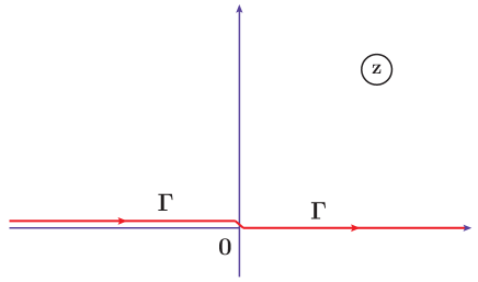
Figure 1: The contour $\Gamma$ in integral (34).

Let us consider the integral

$$\frac{1}{2}\int\limits_{C}\!\!z\,\!g(z^{2})H_{0}^{(1)}(wz)dz\;,$$ (35)

where the closed contour $C$ is a sum of the contour $\Gamma$ and infinite-radius anti-clockwise semi-circle in the upper plane. Since the Hankel function has the asymptotics [16]

$$H_{\nu}^{(1)}(z)=\sqrt{\frac{2}{\pi z}}\,e^{i(4z-2\nu\pi-\pi)/4}\left[1+\mathrm{O}(z^{-1})\right],\quad-\pi<\arg z<2\pi\;,$$ (36)

the integral along the semicircle is zero. By Cauchy’s theorem we pick up the poles of $g(z^{2})$. Q.E.D.

Corollary 1. Under conditions of Theorem 1, the Hankel transform (30) decreases exponentially at large $w$

$$J_{g}(w)=\mathrm{O}(e^{-\gamma w})\;,\quad w\rightarrow\infty\;,$$ (37)

where $\gamma=\min(\mathrm{Im}c_{1},\ldots,\mathrm{Im}c_{k})$. In order to prove this statement, it is enough to use the relation [16]

$$H_{\nu}^{(1)}\left(ze^{i\pi/2}\right)=\frac{2}{\pi i}\,e^{i\nu\pi/2}K_{\nu}(z)\;,$$ (38)

as well as asymptotics of the Macdonald function [16]

$$K_{\nu}(z)\big{|}_{z\gg 1}=\sqrt{\frac{\pi}{2z}}\,e^{-z}[1+\mathrm{O}(z^{-1})]\;,\quad-\frac{3\pi}{2}<\arg z<\frac{3\pi}{2}\;.$$ (39)

We consider two examples of Theorem 1.

Example 1. Let $g(z)$ be a meromorphic function and let $g(x^{2})$ has a simple pole in the upper plane

$$g(x^{2})=\frac{1}{x^{2}+a^{2}}\;.$$ (40)

Then we immediately find from (32) that

$$J_{g}(w)=\pi i\,\frac{xH_{0}^{(1)}(wx)}{x+ia}\bigg{|}_{x=ia}=K_{0}(wa)\;,$$ (41)

where we used Eq. (38) with $\nu=0$.

Example 2. Let $g(z)$ be a meromorphic function and let $g(x^{2})$ has a pole of order $n+1$ ($n\geqslant 1$) in the upper plane

$$g(x^{2})=\frac{1}{(x^{2}+a^{2})^{n+1}}\;.$$ (42)

After changing variable $x=e^{i\pi/2}z$ and taking into account Eq. (38), we obtain

$$J_{g}(w)=\frac{\pi i}{n!}\frac{d^{n}}{dx^{n}}\frac{xH_{0}^{(1)}(wx)}{(x+ia)^{n+1}}\bigg{|}_{x=ia}=(-1)^{n}\frac{2}{n!}\frac{d^{n}}{dz^{n}}\frac{zK_{0}(wz)}{(z+a)^{n+1}}\bigg{|}_{z=a}$$

$$=\frac{(-1)^{n}}{(2a)^{n}n!}\sum_{k=0}^{n-1}\binom{n}{k}\frac{(-1)^{k}}{2^{k}}\,\frac{\Gamma(n+k)(n-k)}{\Gamma(n+1)}\,\frac{1}{z^{n+k}}\frac{d^{n-k}}{dz^{n-k}}\,K_{0}(wz)\big{|}_{z=a},$$ (43)

where $\binom{n}{k}$ is the binomial coefficient. With the use of formula (D.1) derived in Appendix D and relation [16]

$$\left(\frac{1}{z}\frac{d}{dz}\right)^{\!\!m}\!K_{0}(z)=(-1)^{m}z^{-m}K_{m}(z)\;,\quad m=1,2,3,\ldots\;,$$ (44)

we find from (4)

$$J_{g}(w)=\frac{(-1)^{n}}{(2a)^{n}n!}\left(\frac{1}{z}\frac{d}{dz}\right)^{\!\!n}\!\!K_{0}(wz)\big{|}_{z=a}=\frac{1}{n!}\left(\frac{w}{2a}\right)^{\!\!n}K_{n}(wa)\;.$$ (45)

It is a correct expressions for the zero order Hankel transform of function (42) (see Eq. 2.12.4.28 in [18]).

Theorem 2. Let $g(z)$ be an analytic function such that $g(z^{2})$ has a finite number of branch points in the upper half-plane at $a_{1}+ib_{1},\ldots,a_{k}+ib_{k}$, where $a_{i}\neq a_{j}$ for $i\neq j$, and let $g(z)$ satisfies the grows condition of the form

$$|g(z)|=\mathrm{O}(|z|^{-c})\;,\quad c>1/4\;,$$ (46)

for all sufficiently large $|z|$. Then

$$J_{g}(w)=-\frac{1}{2}\sum_{i=1}^{k}\int\limits_{C_{i}}\!\!zg(z^{2})H_{0}^{(1)}(wz)\,dz\;,$$ (47)

where the clockwise contour $C_{i}$ ($i=1,\ldots,k$) comes from infinity along the right side of the branch cut $(a_{i}+ib_{i},a_{i}+i\infty)$, goes around the branch point $a_{i}+ib_{i}$, and then tends to infinity along the left side of this branch cut. For given $C_{i}$, the branch cut of $zg(z^{2})$ is determined by taking the branch of $g(z)$ which is real along the finite section $(a_{i},a_{i}+ib_{i})$ of the imaginary axis.

Proof. Let us complement the contour $\Gamma$ in (34) to a closed contour $C$ in the upper half-plane

$$C=\Gamma+\sum_{i=1}^{k}C_{i}+\sum_{i=1}^{k+1}C_{R_{i}}\;,$$ (48)

where $C_{R_{i}}$ are infinite-radius anti-clockwise contours, while $C_{i}$ are clockwise contours along the sides of the branch cuts $(a_{i}+ib_{i},a_{i}+i\infty)$. By Cauchy’s integral theorem, the integral of the analytic function $z\,\!g(z^{2})H_{0}^{(1)}(wz)$ in the upper half-plane along the closed contour $C$ is equal to zero.

Let $I_{C_{i}}$ ($I_{R_{i}}$) be an integral of this function along the contour $C_{i}$ ($C_{R_{i}}$). All integrals $I_{R_{i}}$ are zero due to condition (46) and asymptotic properties of the Hankel function $H_{0}^{(1)}(z)$ at large $z$ (36). Then formula (47) immediately follows from Eq. (34), Q.E.D.

Corollary 2. Let the function $g(z^{2})$ has a special form

$$g(z^{2})=(z^{2}-z_{1}^{2})^{\alpha_{1}}\ldots(z^{2}-z_{k}^{2})^{\alpha_{k}}f(z^{2})\;,$$ (49)

where $z_{i}=a_{i}+ib_{i}$ with $a_{i}\neq a_{j}$, $b_{i}\neq b_{j}$ for all $i,j=1,2,\ldots,k$, non integer $\alpha_{i}>-1$, and $f(z^{2})$ is a holomorphic function in the upper half-plane. If (49) satisfies asymptotic condition (46) of Theorem 2, then the Hankel transform (30) decreases exponentially at large $w$

$$J_{g}(w)=\mathrm{O}(e^{-\lambda w})\;,\quad w\rightarrow\infty\;,$$ (50)

where $\lambda=\min(b_{1},\ldots,b_{k})$.

Proof. Suppose that $\lambda=b_{p}$, $1\leqslant p\leqslant k$. After changing variables $z=z_{p}+iv$, we obtain from (47), (49) the contribution of the branch cut $(a_{p}+ib_{p},a_{p}+i\infty)$

$$J_{g}^{(p)}(w)=\frac{2}{\pi}\int\limits_{0}^{\infty}\!\!v^{\alpha_{p}}F(v)K_{0}[w(b_{p}+v-ia_{p})]\,dv\;,$$ (51)

where the notation

$$F(v) =iz(z^{2}-z_{1}^{2})^{\alpha_{1}}\ldots(z^{2}-z_{p-1}^{2})^{\alpha_{p-1}}(z^{2}-z_{p+1}^{2})^{\alpha_{p+1}}\ldots(z^{2}-z_{k}^{2})^{\alpha_{k}}$$

$$\times[-i(z+z_{p})]^{\alpha_{p}}f(z^{2})\big{|}_{z=z_{p}+iv}\sin(\pi\alpha_{p})$$ (52)

is introduced. The leading part of the asymptotics of $J_{g}^{(p)}(w)$ is given by

$$J_{g}^{(p)}(w)\big{|}_{w\rightarrow\infty} =\sqrt{\frac{2}{\pi w(b_{p}-ia_{p})}}\,e^{-w(b_{p}-ia_{p})}F(0)\!\int\limits_{0}^{\infty}\!\!v^{\alpha_{p}}e^{-wv}\,dv$$

$$=\sqrt{\frac{2}{b_{p}-ia_{p}}}\,w^{-(\alpha_{p}+3/2)}\,e^{-w(b_{p}-ia_{p})}\,F(0)\;.$$ (53)

As $w$ goes to infinity, contributions from other cuts are non-leading with respect to (4), because $b_{p}<\min(b_{1},\ldots b_{p-1},b_{p+1}\ldots b_{k})$. Q.E.D.

Now we consider four examples of Theorem 2.

Example 3. Let $g(z)$ be an analytic function in the upper half-plane and let $g(x^{2})$ has an integrable branch point in the upper half-plane

$$g(x^{2})=\frac{1}{\sqrt{1+x^{2}}}\;.$$ (54)

It is a particular case of Theorem 2 with $k=1$ $a_{1}=0,b_{1}=1$, and there is the branch cut $(i,i\infty)$ in the upper half-plane. We have (see Eq. 2.12.4.28 in [18])

$$\int\limits_{0}^{\infty}\!\frac{x}{\sqrt{1+x^{2}}}\,J_{0}(wx)\,dx=\frac{1}{w}\,e^{-w}\;.$$ (55)

In Fig. 2 a closed contour is shown which is a sum of the contour $\Gamma$ and contours $C_{i}$, ($i=2,\ldots 6$). In particular, the contour $C_{4}$ is a circle of small radius $r$ centered at $z=i$.

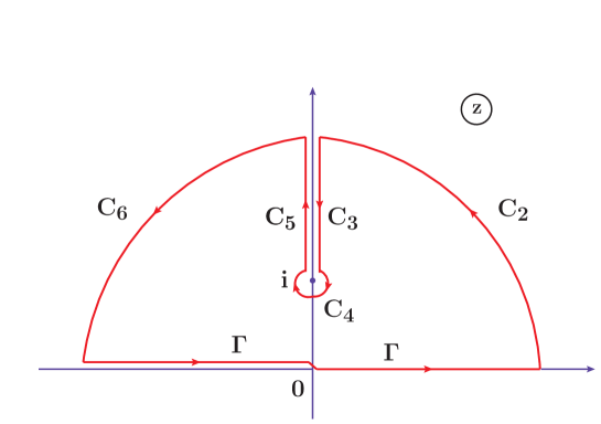
Figure 2: The contour of integration for functions (54), (58).

According to Theorem 2, $J_{g}=-(1/2)(I_{C_{2}}+I_{C_{3}}+I_{C_{4}}+I_{C_{5}}+I_{C_{6}})$. Since $I_{C_{2}}=I_{C_{6}}=0$, and $\lim_{r\rightarrow 0}I_{C_{4}}=0$, we get

$$J_{g}(w)=-\frac{1}{2}\lim_{r\rightarrow 0}(I_{C_{3}}+I_{C_{5}})\;.$$ (56)

Let us change variables $z=ue^{i\pi/2}$. The branch cuts $(\pm i,\pm i\infty)$ in the $z$-plane (see Fig. 2) turn into the branch cuts $(\pm 1,\pm\infty)$ in the $u$-plane. The contours $C_{3}$ and $C_{5}$ have opposite orientations. On the other hand, $\sqrt{1-u^{2}}=-i\sqrt{u^{2}-1}$ at the upper side of the right branch cut $(1,\infty)$, while $\sqrt{1-u^{2}}=i\sqrt{u^{2}-1}$ at its lower side. Thus, $I_{C_{3}}=I_{C_{5}}$. With the use of relation (38) and Eq. 2.16.3.8 in [18], we find that

$$J_{g}(w)=\frac{2}{\pi}\int\limits_{1}^{\infty}\!\frac{u}{\sqrt{u^{2}-1}}\,K_{0}(wu)\,du=\frac{1}{w}\,e^{-w},$$ (57)

in full agreement with Eq. (55) and Corollary 2.

Example 4. Let $g(z)$ be an analytic function in the upper half-plane and let $g(x^{2})$ has a non-integrable branch point there

$$g(x^{2})=\frac{1}{(1+x^{2})^{3/2}}\;.$$ (58)

We get

$$\int\limits_{0}^{\infty}\frac{x}{(1+x^{2})^{3/2}}\,J_{0}(wx)\,dx=e^{-w}.$$ (59)

On the other hand, according to (47), $J_{g}(w)$ is given by the following sum of non-zero contour integrals

$$J_{g}(w)=-\frac{1}{2}\lim_{r\rightarrow 0}(I_{C_{3}}+I_{C_{4}}+I_{C_{5}})\;,$$ (60)

where the contours $C_{i}$ ($i=3,4,5$) are shown in Fig. 2. Since $I_{C_{3}}=I_{C_{5}}$ (see comments after Eq. (56)), changing variables $z=ue^{i\pi/2}$, we obtain

$$I_{C_{3}}+I_{C_{5}} =\frac{4}{\pi}\int\limits_{1+r}^{\infty}\!\frac{u}{(u^{2}-1)^{3/2}}\,K_{0}(wu)\,du$$

$$=\frac{4}{\pi}\frac{1}{\sqrt{r(2+r)}}\,K_{0}[w(1+r)]-\frac{4w}{\pi}\int\limits_{1+r}^{\infty}\!\frac{u}{\sqrt{u^{2}-1}}\,K_{1}(wu)\,du\;.$$ (61)

To calculate the contour integral $I_{C_{4}}$, we put $u=1-re^{i\phi}$, then

$$I_{C_{4}} =\frac{2}{\pi\sqrt{r}}\int\limits_{\pi}^{-\pi}\!d\phi\,e^{-i\phi/2}\frac{1-re^{i\phi}}{(2+re^{i\phi})^{3/2}}\,K_{0}[w(1-re^{i\phi})]\big{|}_{r\rightarrow 0}$$

$$=-\frac{4}{\pi}\frac{1}{\sqrt{2\,r}}\,K_{0}(w)\left[1+\mathrm{O}(r)\right]\;.$$ (62)

As a result, we find in the limit $r\rightarrow 0$

$$J_{g}(w)=\frac{2w}{\pi}\int\limits_{1}^{\infty}\!\frac{u}{\sqrt{u^{2}-1}}\,K_{1}(wu)\,du=e^{-w}.$$ (63)

Thus, Eq. (59) is reproduced. It is in full agreement with Corollary 2.

Example 5. Consider the function

$$g(x^{2})=\frac{1}{\sqrt{x^{4}+2a^{2}x^{2}+b^{4}}}\;,$$ (64)

where $0<a<b$. We have (see Eq. 2.12.6.11 in [18])

$$\int\limits_{0}^{\infty}\!\frac{x}{\sqrt{x^{4}+2a^{2}x^{2}+b^{4}}}\,J_{0}(wx)\,dx=J_{0}\!\left(\!w\sqrt{\frac{b^{2}-a^{2}}{2}}\right)\!K_{0}\!\left(\!w\sqrt{\frac{a^{2}+b^{2}}{2}}\right).$$ (65)

The function (64) has two branch cuts in the upper plane, $(-p+iq,-p+i\infty)$ and $(p+iq,p+i\infty)$, where

$$p=\sqrt{\frac{b^{2}-a^{2}}{2}}\;,\quad q=\sqrt{\frac{b^{2}+a^{2}}{2}}\;.$$ (66)

The contour of integration is shown in Fig. 3.

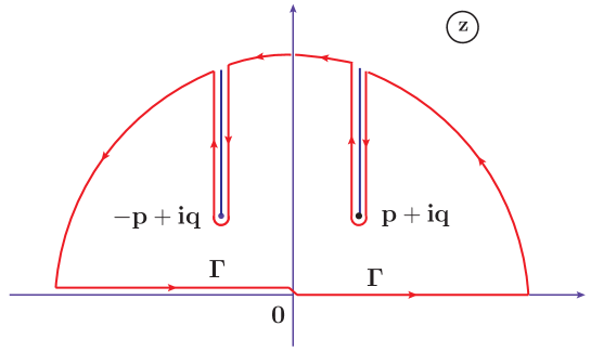
Figure 3: The contour of integration for function (64) with conditions $0<a<b$.

The contribution to $J_{g}(w)$ from the branch cut $(-p+iq,-p+i\infty)$ is given by

$$J_{g}^{(1)}(w)=\frac{2i}{\pi}\int\limits_{q+ip}^{\infty+ip}\!\frac{u}{\sqrt{[(u-q)^{2}+p^{2}][(u+q)^{2}+p^{2}]}}\,K_{0}(wu)\,du\;.$$ (67)

Let us change variables $u=q+ip+z$ ($0<z<\infty$). In order to calculate an asymptotics of $J_{g}^{(1)}(w)$ as $w\rightarrow\infty$, it is enough to put in (67) the asymptotics

$$K_{0}\big{(}w(q+ip+z)\big{)}\big{|}_{w\gg 1}=\sqrt{\frac{\pi}{2w(q+ip)}}\,e^{-w(q+ip-z)}\left[1+\mathrm{O}(w^{-1})\right],$$ (68)

and estimate a rest of the integrand in (67) near the branch point $z=0$

$$\frac{u}{\sqrt{[(u-q)^{2}+p^{2}][(u+q)^{2}+p^{2}]}}\bigg{|}_{z\rightarrow 0}\simeq\frac{1}{2\sqrt{z}}\,\sqrt{\frac{q+ip}{2ipq}}\;.$$ (69)

Then we get

$$J_{g}^{(1)}(w)\big{|}_{w\gg 1} =\frac{1}{2\sqrt{\pi pqw}}\,e^{i\pi/4}\,e^{-w(q+ip)}\int\limits_{0}^{\infty}\frac{dz}{\sqrt{z}}\,e^{-zw}$$

$$=\frac{1}{2w\sqrt{pq}}\,e^{-wq}\,e^{-iw(p-\pi/4)}\;.$$ (70)

Analogously, the contribution to the main asymptotics of $J_{g}(w)$ from the branch cut $(p+iq,p+i\infty)$ is equal to

$$J_{g}^{(2)}(w)\big{|}_{w\gg 1}=\frac{1}{2w\sqrt{pq}}\,e^{-wq}\,e^{iw(p-\pi/4)}\;,$$ (71)

that results in

$$J_{g}(w)\big{|}_{w\gg 1}=\frac{1}{w\sqrt{pq}}\cos\!\left[w\left(p-\frac{\pi}{4}\right)\right]e^{-qw}\,[1+\mathrm{O}(w^{-1})]\;.$$ (72)

Note that we can derive the same asymptotics from the exact formula (65), if we use Eq. (39) and the asymptotics of the Bessel function [16]

$$J_{\nu}(z)\big{|}_{z\gg 1} =\sqrt{\frac{2}{\pi z}}\,\cos\!\left(\frac{4z-2\nu\pi-\pi}{4}\right)\!\left[1+\mathrm{O}(z^{-1})\right],$$

$$-\pi<\arg z<\pi\;.$$ (73)

Assume that, under conditions of Theorem 2, $k\geqslant 2$, and real parts of one pair of the branch points coincide, $a_{n}=a_{m}=a$, while $b_{n}<b_{m}$. Then our formula (47) takes the form

$$J_{g}(w)=-\frac{1}{2}\left[\sum_{\begin{subarray}{c}i=1\\ i\neq n,m\end{subarray}}^{k}\,\int\limits_{C_{i}}\!\!zg(z^{2})H_{0}^{(1)}(wz)\,dz+\int\limits_{C_{nm}}\!\!\!zg(z^{2})H_{0}^{(1)}(wz)\,dz\right],$$ (74)

where $C_{nm}$ is a closed clockwise contour around the finite-length branch cut $(a+ib_{n},a+ib_{m})$. This formula is easily generalized to a case when real parts of two or more pairs of branch points coincide. It is worth to consider a corresponding example.

Example 6. Let us take again function (64), but with the other conditions $0<b<a$. In such a case, $g(z^{2})$ is an analytic function in the upper half-plane with the branch cut $(iu_{1},iu_{2})$, where

$$u_{1}=\sqrt{\frac{a^{2}+b^{2}}{2}}-\sqrt{\frac{a^{2}-b^{2}}{2}}\;,\quad u_{2}=\sqrt{\frac{a^{2}+b^{2}}{2}}+\sqrt{\frac{a^{2}-b^{2}}{2}}\;,$$ (75)

see Fig. 4.

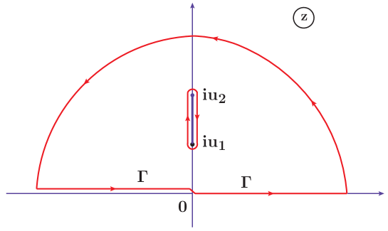
Figure 4: The contour of integration for function (64) with conditions $0<b<a$.

Starting from (74), we come to the following integral (see Eq. 2.16.4.1 in [18])

$$J_{g}(w) =\frac{2}{\pi}\int\limits_{u_{1}}^{u_{2}}\!\frac{u}{\sqrt{(u_{2}^{2}-u^{2})(u^{2}-u_{1}^{2})}}\,K_{0}(wu)\,du\;,$$

$$=I_{0}\!\left(\frac{w(u_{2}-u_{1})}{2}\right)\!K_{0}\!\left(\frac{w(u_{2}+u_{1})}{2}\right),$$ (76)

in agreement with Eq. 2.12.6.10 in [18].

5 Numerical evaluation of total cross section

In this section we numerically calculate the total cross section for a variety of expressions taken for the Born amplitude $A_{\mathrm{B}}(s,t)$. Only Born amplitudes are considered that lead to the correct asymptotics of the eikonal function at large $b$ (18). The main goal is to verify whether our formula approximates $\sigma_{\mathrm{tot}}$ well or not.

In what follows, in order to deal with dimensionless quantities in numerical calculations, it is assumed that the momentum transfer $q=\sqrt{-t}$ and collision energy $\sqrt{s}$ are measured in units of $m_{0}$, where $m_{0}$ has a dimension of mass. Correspondingly, the impact parameter $b$ is measured in units of $m_{0}^{-1}$. We calculate the total cross section at some fixed energy, knowing the Born amplitude at the same $s$.

1. We start from the case when the Born amplitude is a pure imaginary, and it looks like

$$\mathrm{Re}A_{\mathrm{B}}=0\;,\quad\mathrm{Im}A_{\mathrm{B}}=\frac{4\pi as}{(1-t)^{2}}\;,$$ (77)

where $a$ is a $t$-independent quantity to be defined below. It is implied that $a$ may depend on $s$. The imaginary part of the Born amplitude (77) is a meromorphic function of $q$ with the double pole at $q=i$ in the upper half-plane. It corresponds to the following eikonal function

$$\mathrm{Re}\chi(b)=0\;,\quad\mathrm{Im}\chi(b)=a\!\int\limits_{0}^{\infty}\!dqq\,J_{0}(qb)\frac{1}{(1+q^{2})^{2}}=\frac{a}{2}\,bK_{1}(b)\;.$$ (78)

The modified Bessel function $K_{1}(x)$ satisfies condition $\lim_{z\rightarrow 0}[zK_{1}(z)]=1$, and it has asymptotics (39). The function $xK_{1}(x)/2$ is shown in Fig. 5 along with the function $e^{-x}$. Note that (78) is in full agreement with Corollary 1 of Theorem 1 (see also Example 2).

As it was mentioned above, $b$ is measured in units of $m_{0}^{-1}$. It means that in fact

$$\mathrm{Im}\chi(b)=\frac{a}{2}\,m_{0}\mathbf{b}K_{1}(m_{0}\mathbf{b})\;,$$ (79)

where b is the true impact parameter with a dimension of (mass)^-1. If $m_{0}$ depends on $s$, the eikonal function has no factorized form. Its asymptotics is $\sim\exp(-m_{0}\mathbf{b})/\sqrt{m_{0}\mathbf{b}}$.

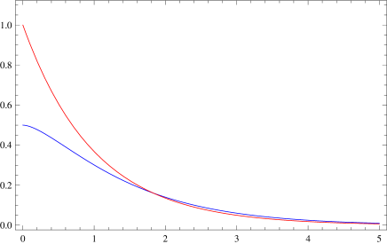
Figure 5: Functions $e^{-x}$ (upper curve) and $xK_{1}(x)/2$ (lower curve).

In the case under consideration, the total cross section is given by

$$\sigma_{\mathrm{tot}}=4\pi\!\int\limits_{0}^{\infty}\!dbb\left\{1-\exp\left[-(ab/2)K_{1}(b)\right]\right\}.$$ (80)

We also have

$$\sigma_{1}=4\pi a\;,\quad\sigma_{2}=-\frac{1}{3}\,\pi a^{2}\;,$$ (81)

$$\sigma_{3}=\frac{2\pi}{3}\,a^{3}\!\int\limits_{0}^{\infty}\!\!dx\frac{x}{(1+x^{2})^{2}}\!\int\limits_{0}^{\infty}\!\!dy\frac{y}{(1+y^{2})^{2}}\!\int\limits_{0}^{\infty}\!\!dz\frac{z}{(1+z^{2})^{2}}\,F_{3}(x,y,z)\;,$$ (82)

where $F_{3}(x,y,z)$ is defined by eq. (B.4).

Let $a=1/4$, then $\mathrm{Im}\chi(b)\leqslant 1/8$ for all $b$ (see Fig. 5). We obtain

$$\sigma_{\mathrm{tot}}=0.979627\,\pi\;,$$ (83)

$$\sigma_{1}+\sigma_{2}=\frac{47}{48}\,\pi\;.$$ (84)

Eq. (Appendix A) gives us

$$\sigma_{3}=0.0014746\;,$$ (85)

and, correspondingly, $\sigma_{1}+\sigma_{2}+\sigma_{3}=3.077615$.

Let us define a relative error

$$\varepsilon^{(n)}=\frac{|\sigma_{\mathrm{tot}}-\sum_{i=1}^{n}\sigma_{i}|}{\sigma_{\mathrm{tot}}}\;.$$ (86)

Then we find

$$\varepsilon^{(2)}=4.7\times 10^{-4}\;,\quad\varepsilon^{(3)}=8.3\times 10^{-6}\;.$$ (87)

As one can see from (87), for moderately small eikonal function ($|\chi(b)|\lesssim 0.1$) the accuracy of our approximate formula (6) is high even if one takes into account only two first terms in it.

2. Let us take a pure real Born amplitude

$$\mathrm{Re}A_{\mathrm{B}}=\frac{\pi s}{(1-t)^{2}}\;,\quad\mathrm{Im}A_{\mathrm{B}}=0\;.$$ (88)

It corresponds to the eikonal function

$$\mathrm{Re}\chi(b)=bK_{1}(b)/8\;,\quad\mathrm{Im}\chi(b)=0\;.$$ (89)

Then calculations give us

$$\sigma_{\mathrm{tot}}=0.0208237\,\pi\;.$$ (90)

The terms $\sigma_{n}$ with odd $n$ are equal to zero, $\sigma_{1}=\sigma_{3}=\sigma_{5}=\ldots=0$, while

$$\sigma_{2}=\frac{\pi}{48}\;,$$ (91)

$$\sigma_{4} =-\frac{\pi}{3\cdot 2^{9}}\!\int\limits_{0}^{\infty}\!\!dx\frac{x}{(1+x^{2})^{2}}\!\int\limits_{0}^{\infty}\!\!dy\frac{y}{(1+y^{2})^{2}}\!\int\limits_{0}^{\infty}\!\!dz\frac{z}{(1+z^{2})^{2}}\!\int\limits_{0}^{\infty}\!\!du\frac{u}{(1+u^{2})^{2}}$$

$$\times F_{4}(x,y,z,u)\;.$$ (92)

To make numerical estimates, we use formula (B.6) and find that

$$\varepsilon^{(2)}=1.7\times 10^{-4}\;,\quad\varepsilon^{(4)}=5.0\times 10^{-5}\;.$$ (93)

It is a surprise that the first nonzero term in expansion (6) results in such a small relative error of $\mathrm{O}(10^{-4})$.

3. Let us study a case when both real and imaginary parts of the Born amplitude are non-zero

$$\mathrm{Re}A_{\mathrm{B}}=\mathrm{Im}A_{\mathrm{B}}=\frac{\pi s}{(1-t)^{2}}\;.$$ (94)

Correspondingly,

$$\mathrm{Re}\chi(b)=\mathrm{Im}\chi(b)=bK_{1}(b)/8\;.$$ (95)

We get the numbers

$$\sigma_{\mathrm{tot}}=0.999098\,\pi\;,$$ (96)

$$\sigma_{1}=\pi=3.141593\;,\quad\sigma_{3}=-0.00294914\;.$$ (97)

Note that $\sigma_{2}=0$ (see Eq. (8)). As a result, we find

$$\varepsilon^{(1)}=9.0\times 10^{-4}\;,\quad\varepsilon^{(3)}=3.7\times 10^{-5}\;.$$ (98)

4. Finally, let us study the case when the real part of the Born amplitude is zero, while its imaginary part is an entire function of variable $q$

$$\mathrm{Re}A_{\mathrm{B}}=0\;,\quad\mathrm{Im}A_{\mathrm{B}}=\pi s\,e^{t/2}\;.$$ (99)

It corresponds to the eikonal function of the form

$$\mathrm{Re}\chi(b)=0\;,\quad\mathrm{Im}\chi(b)=\frac{1}{4}\,e^{-b^{2}/2}\;.$$ (100)

Let us remember that the impact parameter $b$ is measured in units of $m_{0}^{-1}$ (see our comments in the beginning of this section). It means that in fact

$$\mathrm{Im}\chi(b)=\frac{1}{4}\,e^{-(m_{0}\mathbf{b})^{2}/2}\;,$$ (101)

where b is the true impact parameter. Since the parameter $m_{0}$ may depend on $s$, this eikonal function, in general, isn’t factorized.

The asymptotics of $\mathrm{Im}\chi(b)$ is in accordance with Eq. (29). Indeed, our case (99) corresponds to $f(x^{2})=e^{x^{2}/2}$, $w=b$ in (24) and, consequently, to $\xi=1/2$, $\eta=0$ in (25), $\alpha=1/2$ in (28).

We obtain that

$$\sigma_{\mathrm{tot}}=0.940816\,\pi\;,$$ (102)

$$\sigma_{1}=\pi\;,\quad\sigma_{2}=-\frac{\pi}{48}\;,\quad\sigma_{3}=0.010897\;.$$ (103)

Aa in the previous examples, we come to the small relative errors

$$\varepsilon^{(2)}=3.5\times 10^{-3}\;,\quad\varepsilon^{(3)}=1.6\times 10^{-4}\;.$$ (104)

From the above-studied examples we may conclude that for the moderately small eikonal function ($|\chi(b)|\lesssim 0.1$, for all values of the impact parameter $b$), the account of the first three non-zero terms in expansion (6) results in the relative error of $\mathrm{O}(10^{-5})$. Throughout the paper, the notation $\varepsilon=\mathrm{O}(10^{-n})$ means that $\varepsilon$ is a term of the order $(-n)$, i.e. $10^{-n}\leqslant|\varepsilon|<10^{1-n}$.

6 Conclusions

In the present paper the eikonal approximation for the total cross section for the scattering of two unpolarized particles is studied. We have derived the approximate formula in the case when the eikonal function $\chi(s,b)$ is moderately small (see Eqs. (6)–(8), (Appendix A)–(Appendix A)). Namely, we have shown that the total cross section is given by the series of multiple improper integrals of the Born amplitude $A_{B}(s,q)$, $q=\sqrt{-t}$. The advantage of our formula compared to the standard eikonal formulas is that our integrals contain no rapidly oscillating Bessel functions. This circumstance is very important, since integrals with the products of the Bessel functions are very difficult to evaluate numerically because of their poor convergence and oscillatory nature.

At large fixed $s$, the eikonal function decreases exponentially as $b\rightarrow\infty$ (18). On the other hand, it is given by zero order Hankel transform of the function $A_{B}(s,q)$ (3). We have proved two theorems which allow one to relate large $b$ behavior of $\chi(s,b)$ with the analytical properties of the Born amplitude (for details, see Section 4). Six examples of these theorems are presented.

To check the efficiency of our formula, we applied it for the numerical calculations of the total cross section for a number of particular expressions of $A_{B}(s,q)$. Only those Born amplitudes were selected which result in moderately small eikonal functions and lead to the correct asymptotics of $\chi(s,b)$ at large $b$ (18), in accordance with the theorems presented in Sections 3 and 4. Let us underline, we didn’t demand that the resulting eikonal functions should have a factorized form.

The results obtained allow us to make the following conclusions. Provided that $|\chi(s,b)|\lesssim 0.1$ for all $b$, the sum of the first three non-zero terms in expansion (6) approximates the total cross section with the relative error of $\mathrm{O}(10^{-5})$. Higher accuracy can be achieved, if more terms in (6) ($\sigma_{4},\sigma_{5},\ldots$) are taken into account.

Thus, if the Born amplitude is known at some fixed energy $\sqrt{s}$ as a function of the momentum transfer $q$, then our formulas (6)–(8), (Appendix A) enable one to numerically calculate the total cross section for the same $\sqrt{s}$ with the high accuracy.

Appendix A

Here we present the other terms in expansion (6)

$$\sigma_{3}(s) =\frac{1}{2^{5}\pi^{2}s^{3}}\prod_{i=1}^{3}\int\limits_{0}^{\infty}dq_{i}q_{i}\,F_{3}(q_{1},q_{2},q_{3})\Bigg{[}\frac{1}{3}\prod_{i=1}^{3}\mathrm{Im}A_{B}(s,q_{i})$$

$$\ -\mathrm{Im}A_{B}(s,q_{1})\prod_{i=2}^{3}\mathrm{Re}A_{B}(s,q_{i})\Bigg{]},$$ (A.1)

$$\sigma_{4}(s) =\frac{1}{2^{8}\pi^{3}s^{4}}\prod_{i=1}^{4}\int\limits_{0}^{\infty}dq_{i}q_{i}\,F_{4}(q_{1},q_{2},q_{3},q_{4})\Bigg{[}\prod_{i=1}^{2}\mathrm{Im}A_{B}(s,q_{i})\prod_{i=3}^{4}\mathrm{Re}A_{B}(s,q_{i})\,$$

$$-\frac{1}{6}\prod_{i=1}^{4}\mathrm{Re}A_{B}(s,q_{i})-\frac{1}{6}\prod_{i=1}^{4}\mathrm{Im}A_{B}(s,q_{i})\Bigg{]},$$ (A.2)

$$\sigma_{5}(s) =\frac{1}{3\cdot 2^{10}\pi^{4}s^{5}}\prod_{i=1}^{5}\int\limits_{0}^{\infty}dq_{i}q_{i}\,F_{5}(q_{1},q_{2},q_{3},q_{4},q_{5})\Bigg{[}\frac{1}{10}\prod_{i=1}^{5}\mathrm{Im}A_{B}(s,q_{i})$$

$$+\frac{1}{2}\,\mathrm{Im}A_{B}(s,q_{1})\,\prod_{i=2}^{5}\mathrm{Re}A_{B}(s,q_{i})$$

$$-\prod_{i=1}^{3}\mathrm{Im}A_{B}(s,q_{i})\prod_{i=4}^{5}\mathrm{Re}A_{B}(s,q_{i})\Bigg{]},$$ (A.3)

$$\sigma_{6}(s) =\frac{1}{3\cdot 2^{14}\pi^{5}s^{6}}\prod_{i=1}^{6}\int\limits_{0}^{\infty}dq_{i}q_{i}\,F_{6}(q_{1},q_{2},q_{3},q_{4},q_{5},q_{6})\Bigg{[}\!-\frac{1}{15}\prod_{i=1}^{6}\mathrm{Im}A_{B}(s,q_{i})$$

$$+\frac{1}{15}\prod_{i=1}^{6}\mathrm{Re}A_{B}(s,q_{i})-\prod_{i=1}^{2}\mathrm{Im}A_{B}(s,q_{i})\prod_{i=3}^{6}\mathrm{Re}A_{B}(s,q_{i})$$

$$+\prod_{i=1}^{4}\mathrm{Im}A_{B}(s,q_{i})\prod_{i=5}^{6}\mathrm{Re}A_{B}(s,q_{i})\Bigg{]}.$$ (A.4)

The explicit expressions for the functions $F_{i}$ ($i=3,4,5,6$) are given by Eqs. (B.4), (B.6), (B.10) and (B.11) in Appendix B.

Appendix B

Let us define the integral with the product of several Bessel functions

$$F_{n}(a_{1},\ldots,a_{n})=\int\limits_{0}^{\infty}\!\!dxx\prod_{k=1}^{n}J_{0}(a_{k}x)\;,$$ (B.1)

where $a_{k}>0$, $n\geqslant 2$, $k=1,\ldots,n$. The case $n=2$ is well-known (see Eq. 6.512.8. in [19])

$$F_{2}(a,b)=\int\limits_{0}^{\infty}\!\!dxxJ_{0}(ax)J_{0}(bx)=\frac{1}{a}\,\delta(a-b)\;.$$ (B.2)

The integral with the product of three Bessel functions $J_{0}(x)$ ($a,b,c>0$),

$$F_{3}(a,b,c)=\int\limits_{0}^{\infty}\!\!dxxJ_{0}(ax)J_{0}(bx)J_{0}(cx)\;,$$ (B.3)

is given by the formula (see Eq. 13.46(3) in [17], as well as Eqs. 2.12.42.14., 2.12.42.15. in [18])

$$F_{3}(a,b,c)=\left\{\begin{array}[]{cc}\displaystyle{\frac{1}{2\pi\Delta_{3}}},&\Delta_{3}^{2}>0\;,\\ \\ 0,&\Delta_{3}^{2}<0\;,\end{array}\right.$$ (B.4)

where

$$16\Delta_{3}^{2}=[c^{2}-(a-b)^{2}][(a+b)^{2}-c^{2}]\;.$$ (B.5)

Note that expression (B.4) is divergent if $\Delta_{3}^{2}=0$ (it takes place when one of the parameters is equal to the sum of the others, say, $c=a+b>0$).

The complete expression for $F_{4}(a,b,c,d)$ was derived in [8].

$$F_{4}(a,b,c,d)=\left\{\begin{array}[]{cl}\displaystyle{\frac{1}{\pi^{2}\Delta_{4}}\,\mathrm{K}\!\left(\frac{\sqrt{abcd}}{\Delta_{4}}\right)},&\Delta_{4}^{2}>abcd\;,\\ \\ \displaystyle{\frac{1}{\pi^{2}\sqrt{abcd}}\,\mathrm{K}\!\left(\frac{\Delta_{4}}{\sqrt{abcd}}\right)},&0<\Delta_{4}^{2}<abcd\;,\\ \\ \displaystyle{\frac{1}{2\pi\sqrt{abcd}}}&\Delta_{4}^{2}=0\;,\\ \\ 0,&\Delta_{4}^{2}<0\;,\end{array}\right.$$ (B.6)

where $a,b,c,d>0$,

$$16\Delta_{4}^{2}=(a+b+c-d)(a+b+d-c)(a+c+d-b)(b+c+d-a)\;,$$ (B.7)

and

$$\mathrm{K}(k)=\int\limits_{0}^{1}\!\frac{dt}{\sqrt{(1-t^{2})(1-k^{2}t^{2})}}$$ (B.8)

is the complete elliptic integral of the first kind ($0\leqslant k<1$) [20]. The quantity $F_{4}(a,b,c,d)$ (B.6) is not defined if $\Delta_{4}^{2}=abcd$, since $\mathrm{K}(k)$ diverges as $k\rightarrow 1$ [20]

$$\mathrm{K}(k)\big{|}_{k\rightarrow 1}\simeq\ln(4/\sqrt{1-k^{2}})\;.$$ (B.9)

Nevertheless, since $F_{4}(a,b,c,d)$ will be used only as a part of integrands, we can safely put $F_{4}(a,b,c,d)=0$ for $\Delta_{4}^{2}=abcd$ in numerical calculations.

Finally, the following expressions were obtained in [8] ($a,b,c,d,e,f>0$)

$$F_{5}(a,b,c,d,e) =\int\limits_{0}^{\infty}\!dt\,t\,F_{3}(a,b,t)\,F_{4}(c,d,e,t)\;,$$ (B.10)

$$F_{6}(a,b,c,d,e,f) =\int\limits_{0}^{\infty}\!dt\,t\,F_{4}(a,b,c,t)\,F_{4}(d,e,f,t)\;,$$ (B.11)

where $F_{3}(a_{1},a_{2},a_{3})$ and $F_{4}(a_{1},a_{2},a_{3},a_{4})$ are defined by formulas (B.4) and (B.6), respectively. By doing in the same way, one can express integral (B.1) for $n>6$ and $a_{k}>0$, $k=1,\ldots,n$, as a $(n-3)$-dimensional integral of algebraic functions. Let us note that $F_{n}(a_{1},\ldots,a_{n})=0$ for $n\geqslant 2$, if $a_{n}>a_{1}+a_{2}+\ldots a_{n-1}$.

Appendix C

Here we give a simple proof of formula (15). The differential equation for the Legendre function of the first kind $u(z)=P_{\nu}^{-\mu}(z)$ looks like [13]

$$(1-z^{2})\frac{d^{2}}{dz^{2}}\,u(z)-2z\frac{d}{dz}\,u(z)+\left[\nu(\nu+1)-\frac{\mu^{2}}{1-z^{2}}\right]\!u(z)=0\;.$$ (C.1)

Let us change variables

$$z=\cos\frac{x}{\nu}\;.$$ (C.2)

In the limit $\nu\gg 1\gg x$, we get

$$z\frac{d}{dz}\simeq-\frac{\nu^{2}}{x}\,\frac{d}{dx}\;,\quad(1-z^{2})\frac{d^{2}}{dz^{2}}\simeq\nu^{2}\!\left[\frac{d^{2}}{dx^{2}}-\frac{1}{x}\frac{d}{dx}\right],$$ (C.3)

and differential equation (C.1) takes the form

$$x^{2}\frac{d^{2}}{dx^{2}}\,u(x)+x\frac{d}{dx}\,u(x)+(x^{2}-\mu^{2})u(x)=0\;,$$ (C.4)

which is Bessel’s equation [16]. It means that

$$\lim_{\nu\rightarrow\infty}\,P_{\nu}^{-\mu}\!\left(\cos\frac{x}{\nu}\right)=c_{1}J_{\mu}(x)+c_{2}Y_{\mu}(x)\;,$$ (C.5)

where $c_{1},c_{2}$ are constants. The singular solution to the Bessel equation $Y_{\mu}(x)$ is ruled out, since $P_{\nu}^{-\mu}\!\left(\cos\frac{x}{\nu}\right)$ is regular at $x=0$. So, $c_{2}=0$. We obtain

$$P_{\nu}^{-\mu}\!\left(\cos\frac{x}{\nu}\right)\Big{|}_{x\ll 1\ll\nu}=\frac{1}{\Gamma(1+\mu)}\left(\frac{x}{2}\right)^{\!\mu}=J_{\mu}(x)\Big{|}_{x\ll 1}\;,$$ (C.6)

that results in $c_{1}=1$, and Eq. (15) is reproduced.

Appendix D

Let us prove the formula

$$\left(\frac{1}{z}\frac{d}{dz}\right)^{\!\!n}=\sum_{k=0}^{n-1}\frac{(-1)^{k}}{2^{k}}\frac{\Gamma(n+k)}{\Gamma(k+1)\Gamma(n-k)}\frac{1}{z^{n+k}}\frac{d^{n-k}}{dz^{n-k}}\;,$$ (D.1)

where $n=1,2,3,\ldots$, using mathematical induction. It is evidently that our statement (D.1) is valid for $n=1$. Let us assume that it holds for some integer $n=m>1$,

$$P(m)=\left(\frac{1}{z}\frac{d}{dz}\right)^{\!\!m}=\sum_{k=0}^{m-1}\frac{(-1)^{k}}{2^{k}}\frac{\Gamma(m+k)}{\Gamma(k+1)\Gamma(m-k)}\frac{1}{z^{m+k}}\frac{d^{m-k}}{dz^{m-k}}\;.$$ (D.2)

Then we find using Eq. (D.2)

$$\left(\frac{1}{z}\frac{d}{dz}\right)^{\!\!m+1} =\sum_{k=0}^{m-1}\frac{(-1)^{k}}{2^{k}}\frac{\Gamma(m+k)}{\Gamma(k+1)\Gamma(m-k)}$$

$$\times\left[\frac{1}{z^{m+1+k}}\frac{d^{m+1-k}}{dz^{m+1-k}}-(m+k)\frac{1}{z^{m+2+k}}\frac{d^{m-k}}{dz^{m-k}}\right]$$

$$=\sum_{k=0}^{m}\frac{(-1)^{k}}{2^{k}}\frac{\Gamma(m+1+k)}{\Gamma(k+1)\Gamma(m+1-k)}\frac{1}{z^{m+1+k}}\frac{d^{m+1-k}}{dz^{m+1-k}}$$

$$=P(m+1)\;.$$ (D.3)

So, the inductive case holds. Consequently, formula (D.1) is valid for all integer $n\geqslant 1$. Q.E.D.

References

- [1] G. Molière, Theorie der Streuung schneller geladener Teilchen I. Einzelstreuung am abgeschirmten Coulomb-Feld (in German), Z. Naturforsch. A 2, 133 (1947); Theorie der Streuung schneller geladener Teilchen II. Mehrfach- und Vielfachstreuung (in German), Z. Naturforsch. A 3, 78 (1948).
- [2] R.J. Glauber, in Lectures in Theoretical Physics, ed. W.E. Brittin and L.G. Dunham, New York, Vol. 1, 1959, p. 315.
- [3] H. Cheng and T.T. Wu, High-Energy Elastic Scattering in Quantum Electrodynamics, Phys. Rev. Lett. 22, 666 (1969); Impact Factor and Exponentiation in High-Energy Scattering Processes, Phys. Rev. 186, 1611 (1969).
- [4] A.A. Logunov, A.N. Tavkhelidze, Quasi-optical approach in quantum field theory, Nuovo Cim. 29, 380 (1963).
- [5] P.D.B. Collins, An introduction to Regge theory & high energy physics, Cambridge University Press, 1977.
- [6] S.K. Lucas, Evaluating infinite integrals involving products of Bessel functions of arbitrary order, J. Comput. Appl. Math. 64, 269 (1995).
- [7] J.V. Deun and R. Cools, Integrating products of Bessel functions with an additional exponential or rational factor, Comp. Phys. Comm. 178, 578 (2008).
- [8] A.V. Kisselev, Approximate formulas for moderately small eikonal amplitudes, Teor. Math. Phys. 188, 2, 1197 (2016).
- [9] M. Abramowitz and I.A. Stegun (Eds.), Handbook of Mathematical Functions with Formulas, Graphs, and Mathematical Tables, Tenth printing, Dover, New York, 1972.
- [10] E.T. Whittaker, G.N. Watson, A Course of Modern Analysis, 4th edition, Cambridge University Press, 1927.
- [11] F.G. Mehler, Über die Vertheilung der statischen Elektricität in einem von zwei Kugelkalotten begrenzten Körper (in German), J. für die Reine und Angewandte Math. 68, 134 (1868); Notiz über die Dirichlet’schen Integralausdrücke für die Kugelfunktion und über eine analoge Integralform für die Zylinderfunktion (in German), Math. Ann. 5, 141 (1872).
- [12] G. Szegő, Orthogonal polynomials. American Mathematical Society, Providence, R.I., fourth edition, 1975.
- [13] Higher Transcendental Functions. Vol. 1. By the staff of the Bateman manuscript project (A. Erdélyi, Editor; W. Magnus, F. Oberhettinger, F.G. Tricomi, Associates), McGraw-Hill Book Company, New York, 1953.
- [14] A.V. Kisselev, Ramanujan’s Master Theorem and two formulas for zero-order Hankel transform, arXiv:math.CA/1801.06390.
- [15] C.L. Frenzen and R. Wong, A Note on Asymptotic Evaluation of Some Hankel Transforms, Math. Comp. 45, 537 (1985).
- [16] Higher Transcendental Functions. Vol. 2. By the staff of the Bateman manuscript project (A. Erdélyi, Editor; W. Magnus, F. Oberhettinger, F.G. Tricomi, Associates), McGraw-Hill Book Company, New York, 1953.
- [17] G.N. Watson, A Treatise on the Theory of Bessel Functions, 2nd edition, Cambridge University Press, 1995.
- [18] A.P. Prudnikov, Yu.A. Brychkov and O.I. Marichev, Integrals and Series, Vol. 2: Special Functions, Gordon & Breach Sci. Publ., New York, 1986.
- [19] I.S. Gradshteyn and I.M. Ryzhik, Table of Integrals, Series, and Products, 7th edition, Academic Press, New York, 2007.
- [20] Higher Transcendental Functions. Vol. 3. By the staff of the Bateman manuscript project (A. Erdélyi, Editor; W. Magnus, F. Oberhettinger, F.G. Tricomi, Associates), McGraw-Hill Book Company, New York, 1955.