How Thermal Inflation can save Minimal Hybrid Inflation in Supergravity

Abstract

Minimal hybrid inflation in supergravity has been ruled out by the 2015 Planck observations because the spectral index of the produced curvature perturbation falls outside observational bounds. To resurrect the model, a number of modifications have been put forward but many of them spoil the accidental cancellation that resolves the $\eta$-problem and require complicated Kähler constructions to counterbalance the lost cancellation. In contrast, in this paper the model is rendered viable by supplementing the scenario with a brief period of thermal inflation, which follows the reheating of primordial inflation. The scalar field responsible for thermal inflation requires a large non-zero vacuum expectation value (VEV) and a flat potential. We investigate the VEV of such a flaton field and its subsequent effect on the inflationary observables. We find that, for large VEV, minimal hybrid inflation in supergravity produces a spectral index within the 1-sigma Planck bound and a tensor-to-scalar ratio which may be observable in the near future. The mechanism is applicable to other inflationary models.

1 Introduction

The precision of the latest observational data from the Planck satellite is so high that it excludes several families of well motivated and thoroughly explored inflationary models [1]. A prominent example is minimal hybrid inflation.

Hybrid inflation was introduced by Linde [2] to employ sub-Planckian field values whilst avoiding ‘unnaturally’ tiny couplings. A supergravity (SUGRA) version of the model [3] has the neat feature that a minimal Kähler potential $K$, apart from rendering the fields canonically normalised, avoids excessive Kähler corrections due to an accidental cancellation.

Inflationary model-building in SUGRA suffers from the infamous $\eta$-problem, because the scalar potential is proportional to $e^{K/m_{P}^{2}}$ which results in $\eta=K^{\prime\prime}+\cdots$, where $\eta$ is the second slow-roll parameter and the primes denote derivatives with respect to the inflaton. For canonical fields $K^{\prime\prime}=1$ so, in general, slow-roll is spoilt. However, for hybrid inflation with a minimal Kähler potential a term in the ellipsis cancels $K^{\prime\prime}$ and allows $\eta\ll 1$ during inflation.

It was rather disappointing that the Planck observations killed the minimal hybrid model. This is why many authors put forward modifications, which produce observables within the allowed ranges but at the expense of the above accidental cancellation. Thus, elaborate Kähler constructions were introduced to ensure slow-roll (e.g. see Ref. [4] and references therein - but also see Ref. [5]).

Another proposal is Double Inflation [6], which retains the accidental cancellation mentioned above, and utilises a second period of inflation, such that the number of e-folds of remaining primordial inflation when the cosmological scales exit the horizon is reduced. As a result, the inflationary observables are affected in a way that renders them compatible with observations. In Double Inflation, however, the inflationary model is modified to enable the second stage of inflation (which follows directly after the first stage), when the field follows a semi-shifted path in configuration space. Thus, the model is no longer minimal.

In this paper we propose a mechanism which manages to render the model compatible with observations whilst retaining the neat feature of the accidental cancellation of minimal hybrid inflation in SUGRA. In contrast to Ref. [6], we do not modify the primordial inflation model. We simply consider that, after reheating, there is a period of thermal inflation due to some flaton scalar field. The mechanism operates with any suitable flaton of mass $\sim\,$1 TeV. As with Double Inflation, our mechanism dilutes unwanted relics, possibly formed at the end of minimal hybrid inflation in SUGRA.

We use natural units, for which $c=\hbar=1$ and $m_{P}^{-2}=8\pi G$, with $m_{P}=2.43\times 10^{18}\,$GeV being the reduced Planck mass.

2 Minimal Hybrid Inflation in Supergravity

Hybrid inflation in SUGRA is achieved with the superpotential:

$$W=\kappa S(\Phi\bar{\Phi}-M^{2})+\cdots$$ (1)

where the dots denote Planck-suppressed non-renormalisable operators, $\Phi,\bar{\Phi}$ are a pair of singlet lefthanded superfields and $S$ is a gauge singlet superfield which acts as the inflaton. The flatness of the inflationary trajectory is guaranteed by a U(1) R-symmetry on $S$. The parameters $\kappa$ and $M$ are made positive with field redefinitions, where $M\sim 10^{16}\,$GeV is the scale of a grand unified theory (GUT) and $\kappa\leq 1$ is a dimensionless coupling constant. The supersymmetric minimum is at $\langle\Phi\rangle=\langle\bar{\Phi}\rangle=M$ and $\langle S\rangle=0$. We also consider a minimal Kähler potential for the fields:

$$K=|\Phi|^{2}+|\bar{\Phi}|^{2}+|S|^{2}$$ (2)

Then the F-term scalar potential is:

$$V_{F}=\kappa^{2}|M^{2}-\Phi\bar{\Phi}|^{2}+\kappa^{2}|S^{2}|(|\Phi|^{2}+|\bar{\Phi}|^{2})+\cdots$$ (3)

where the dots denote Planck-suppressed terms and we consider that the fields are sub-Planckian.

When $|\langle\Phi\rangle|=|\langle\bar{\Phi}\rangle|$ the D-terms vanish. Since the soft-breaking terms are negligible near the inflation scale (the GUT scale), the scalar potential is $V=V_{F}+\Delta V$, where $\Delta V$ is the Coleman-Weinberg one-loop radiative correction:

$$\Delta V\simeq\frac{\kappa^{4}M^{4}}{16\pi^{2}}\ln\frac{\kappa^{2}|S|^{2}}{\Lambda^{2}}\,,$$ (4)

where $\Lambda$ is some renormalisation scale. By suitable rotations in field space we write $\sigma=\sqrt{2}S$ and $\Phi=\bar{\Phi}=\varphi/2$, where $\sigma$, $\varphi$ are canonically normalised real scalar fields [7].

From Eq. (3), the mass-squared for the waterfall field $\varphi$ is

$$m_{\varphi}^{2}\simeq\kappa^{2}(|S|^{2}-M^{2})\,.$$ (5)

Hence, when $\sigma<\sigma_{c}\equiv\sqrt{2}M$, the field becomes tachyonic. For $\sigma>\sigma_{c}$ the potential is minimised for $\Phi=\bar{\Phi}=0$ (i.e. $\varphi=0$) and inflation is driven by the false vacuum density $\kappa^{2}M^{4}$. Inflation ends abruptly at the waterfall when $\sigma=\sigma_{c}$. Then, during inflation, the potential becomes

$$V=\kappa^{2}M^{4}+\frac{\kappa^{4}M^{4}}{8\pi^{2}}\ln\left(\frac{\kappa\sigma}{\sqrt{2}\Lambda}\right)\,.$$ (6)

where the second term is subdominant but provides a slope along the inflationary valley, necessary for slow-roll. One of the advantages of the model is that, by keeping the minimal Kähler potential, the accidental cancellation still avoids the $\eta$-problem, otherwise endemic in SUGRA inflation.

The slow-roll parameters are:

$$\epsilon=\frac{m_{P}^{2}}{2}\left(\frac{V^{\prime}}{V}\right)^{2}=\frac{\kappa^{4}}{128\pi^{4}}\left(\frac{m_{P}}{\sigma}\right)^{2}\,,$$ (7)

$$\eta=m_{P}^{2}\frac{V^{\prime\prime}}{V}=-\frac{\kappa^{2}}{8\pi^{2}}\left(\frac{m_{P}}{\sigma}\right)^{2}\,,$$ (8)

where the prime denotes derivative with respect to the inflaton $\sigma$. For the spectral index of the density perturbations we have

$$n_{s}-1=-\frac{\kappa^{2}}{4\pi^{2}}\left(1+\frac{3\kappa^{2}}{16\pi^{2}}\right)\left(\frac{m_{P}}{\sigma}\right)^{2}\,,$$ (9)

while the tensor to scalar ratio is given by the consistency condition as $r=16\epsilon$. Expressing the above in terms of the remaining inflation e-folds $N$, using

$$\Big{(}\frac{\sigma}{m_{P}}\Big{)}^{2}=2\Big{(}\frac{M}{m_{P}}\Big{)}^{2}+\frac{\kappa^{2}}{4\pi^{2}}N\,,$$ (10)

where $\sigma_{c}^{2}\equiv 2M^{2}$, we find:

$$r=16\epsilon\simeq\frac{\kappa^{2}}{2\pi^{2}}\frac{1}{N}$$ (11)

and

$$n_{s}-1=2\eta-6\epsilon\simeq-\frac{1}{N}\,.$$ (12)

Examining Eqs. (11) and (12) with $\kappa=0.1$ and $N=60\;(50)$ gives us $r=8\times 10^{-6}$ $(1\times 10^{-5})$ and $n_{s}=0.983\;(0.980)$. Whilst $r$ is well beneath the Planck upper bound, but as yet unobservable, $n_{s}$ is clearly above the upper 2-$\sigma$ bound of the Planck observations [1]. Therefore, the model appears to be excluded. To account for this problem, many authors suggested modifications of the theoretical setup. However, these lost the accidental cancellation that resolved the $\eta$-problem. Consequently, this required the further introduction of complicated versions of the Kähler potential to keep Kähler corrections under control. In this paper, we propose a simpler tactic. By examining Eqs. (11) and (12) we notice that a lower value of $N$ can bring $n_{s}$ within the Planck bounds. Furthermore, it may also increase $r$ to the point of observability.

3 Thermal Inflation

3.1 The model

We will assume the existence of a so-called flaton field, which can realise thermal inflation. This is a brief period of inflation lasting up to $N_{T}\simeq 17$ e-folds, occurring shortly after reheating from primordial inflation. A bout of thermal inflation occurs from the moment when the scalar potential dominates the thermal bath density, with the field being held on top of a false vacuum, until the moment when a phase transition releases the field from the false vacuum and sends it towards its true vacuum expectation value (VEV). Therefore, thermal inflation requires a scalar field with a large VEV and a flat potential; such a field is called a flaton [8]. Typically, a flaton field corresponds to a supersymmetric flat direction, lifted by a soft mass $\sim\,$1 TeV.

Now, the number of e-folds before the end of primordial inflation that correspond to the exit of the cosmological scales, $N$, can be reduced by $N_{T}$. By investigating the effect of the VEV of the thermal flaton on $N_{T}$ we can determine $N$ anew and hence $r(N)$ and $n_{s}(N)$ for inflationary models. We find that this may render minimal hybrid inflation in SUGRA viable.

The zero temperature flaton potential and its VEV are:

$$V=V_{0}-\frac{1}{2}m^{2}\phi^{2}+\frac{\lambda}{[2(n+2)]!}\frac{\phi^{2(n+2)}}{m_{P}^{2n}}\,,$$ (13)

$$\langle\phi\rangle=\Big{[}\frac{\lambda}{(2n+3)!}\Big{]}^{-\frac{1}{2(n+1)}}(m_{P}^{n}m)^{\frac{1}{n+1}}\,,$$ (14)

where $n>0$ is an integer. For a given $m$, a large VEV is attained with large $n$. When $n\rightarrow\infty$ we have $\langle\phi\rangle\rightarrow m_{P}$. This case may correspond to a string modulus, whose otherwise flat potential may vary over $m_{P}$ distances in field space [8].

From the above, it is easy to show that the flaton mass-squared is

$$V^{\prime\prime}(\langle\phi\rangle)=2(n+1)m^{2}$$ (15)

Also, because $V(\langle\phi\rangle)=0$ we find:

$$V_{0}=\frac{1}{2}\Big{(}\frac{n+1}{n+2}\Big{)}m^{2}\langle\phi\rangle^{2}\,.$$ (16)

Thus, the energy scale of thermal inflation is, $V_{0}^{1/4}\sim\sqrt{m\langle\phi\rangle}$.

However, the flaton field interacts strongly with the thermal bath, which introduces an additional, sizeable, term in Eq. (13) of the form $\frac{1}{2}g^{2}T^{2}\phi^{2}$, where $g$ is the coupling to the thermal bath and $T$ is the temperature [8]. Thus, the effective mass-squared is now

$$m_{\rm eff}^{2}=g^{2}T^{2}-m^{2}$$ (17)

For high temperatures, $m_{\rm eff}^{2}$ is positive and the flaton is driven to zero, where the potential in Eq. (13) is $V(0)=V_{0}$. Thermal inflation begins when $V_{0}$ overwhelms the density of the thermal bath, $\rho_{T}=\frac{\pi^{2}}{30}g_{*}T^{4}$, where $g_{*}$ is the effective relativistic degrees of freedom. Thus, the temperature at the onset of thermal inflation is

$$T_{1}=\Big{(}\frac{30}{\pi^{2}g_{*}}\Big{)}^{\frac{1}{4}}V_{0}^{1/4}\sim V_{0}^{1/4}\,.$$ (18)

Thermal inflation continues as long as the flaton field is kept on top of the false vacuum by the thermal interaction term. However, the thermal bath is exponentially depleted, so the temperature drops enough that $m_{\rm eff}^{2}$ becomes tachyonic and the flaton is released towards its VEV. This event terminates thermal inflation, and corresponds to the temperature

$$T_{2}=m/g\,.$$ (19)

The e-folds of thermal inflation are

$$N_{T}=\ln\Big{(}\frac{T_{1}}{T_{2}}\Big{)}\simeq\ln\frac{gV_{0}^{1/4}}{m}\simeq\frac{1}{2}\ln\left(\frac{\langle\phi\rangle}{m}\right)\,,$$ (20)

where we considered $g\sim 1$. From the above we see that the flaton VEV determines $N_{T}$.

3.2 Some particulars of Thermal Inflation

Before continuing, we briefly discuss some particular issues regarding thermal inflation. First, we consider whether the flaton potential is given by Eq. (13) during inflation as well as in the vacuum. We also comment on the expectation value of the flaton field during and after inflation.

If the flaton were light (with sub-Hubble mass) during inflation then it would undergo particle production and develop a non-zero condensate. After the end of inflation and before reheating, however, while the inflaton field is oscillating, there is a thermal bath with temperature $T\sim(m_{P}^{2}\Gamma H)^{1/4}$ [9], which is bigger that the reheating temperature $\sim\sqrt{m_{P}\Gamma}$ ($\Gamma$ being the inflaton perturbative decay rate) that reduces in time as $T\propto t^{-1/4}$, while $H\propto 1/t$. The thermal mass of the flaton is $\sim T$ (taking $g\sim 1$), which means that the field becomes heavy (with super-Hubble mass) and rolls towards zero when the Hubble parameter is $H_{x}\sim(m_{P}^{2}\Gamma)^{1/3}>\Gamma$, i.e. well before reheating, as it is straightforward to show.

In SUGRA theories, however, a scalar field receives a mass of order $H$ [10], which is the source of the $\eta$-problem. This means that it is not light during inflation, but rolls to zero well before inflation ends. The Hubble-scale mass becomes negligible before reheating (when $H(t)=H_{x}$) and is irrelevant during thermal inflation.

Another issue is the following. One might worry that the coupling of the flaton to the thermal bath, which also couples to the waterfall field, may affect the potential in inflation. Note, however, that the waterfall field is zero during inflation, as most probably is the flaton as well (due to SUGRA corrections), while the particles of the thermal bath are absent because the latter is inflated away. Thus, we do not expect the potential in inflation to be affected by any non-zero contributions due to the flaton field.

Finally, the phase transition which ends thermal inflation can produce unwanted dangerous relics such as domain walls. One way to circumvent this problem is to gauge the thermal flaton such that the end of thermal inflation produces only harmless local cosmic strings, whose energy scale $V_{0}^{1/4}$ is too low to have any cosmological significance. The U(1) Goldstone boson is eaten by the gauge field, which promptly decays assuming a large mass due to the VEV of the flaton.

3.3 The impact on $N$

To find the impact on $N$ we need to consider when reheating occurred. The remaining number of e-folds of primordial inflation when the cosmological scales exit the horizon is

$$N=62.8+\ln\Big{(}\frac{k}{a_{0}H_{0}}\Big{)}+\frac{1}{3}\ln\Big{(}\frac{g_{*}}{106.75}\Big{)}+\ln\Big{(}\frac{V_{\rm end}^{1/4}}{10^{16}\,{\rm GeV}}\Big{)}-\Delta N-N_{T}\,,$$ (21)

where $k=0.05\,$Mpc^-1 is the pivot scale and $(a_{0}H_{0})^{-1}$ is the comoving Hubble radius today. In the above, $V_{\rm end}^{1/4}$ is the energy scale at the end of inflation (typically the GUT scale) and

$$\Delta N=\frac{1}{3}\ln\left(\frac{V_{\rm end}^{1/4}}{T_{\rm reh}}\right)\,,$$ (22)

which is introduced by assuming that, between the end of inflation and reheating, the Universe is dominated by the inflaton condensate, that coherently oscillates in a quadratic potential, near its global minimum. Inefficient reheating can lead to low values for $T_{\rm reh}$.

To minimise $N$, we assume the lowest possible reheating temperature. With a subsequent period of thermal inflation, the reheating from primordial inflation must have completed before the thermal inflation initiates. Hence, $T_{\rm reh}^{4}\geq V_{0}$. Therefore, the minimum $N$ is achieved when

$$\Delta N\simeq\frac{1}{3}\ln\left(\frac{V_{\rm end}^{1/4}}{\sqrt{m\langle\phi\rangle}}\right)\,,$$ (23)

In view of the above, $N$ can be minimized by the combined effect of low reheating and subsequent thermal inflation by the number of e-folds given by

$$\Delta N+N_{T}\simeq\frac{1}{3}\ln\left(\frac{V_{\rm end}^{1/4}\langle\phi\rangle}{m^{2}}\right)\simeq\frac{1}{3}\ln\left[\frac{V_{\rm end}^{1/4}}{m}\left(\frac{m_{P}}{m}\right)^{\frac{n}{n+1}}\right]$$ (24)

where we used that $\langle\phi\rangle\sim(m_{P}^{n}m)^{1/(n+1)}$ in accordance to Eq. (14) (we assumed $\lambda\sim 1$).

4 Impact of Varying $\langle\phi\rangle$ on Hybrid Inflation

Eq. (24) suggests that to minimise $N$ we need to reduce both $m$ and $n$ as much as possible. We take the value $m=1$TeV for the flaton tachyonic mass. This results in a a mass $\geq 2$ TeV as suggested by Eq. (15) for $n\geq 1$, which is the lowest allowed by LHC.

Table 1 shows the results of varying $\langle\phi\rangle$, thereby determining the range of $N$ which can be used to calculate $r$ and $n_{s}$ for given inflationary models.

$\langle\phi\rangle$ (GeV)	$N_{T}$	$N+N_{T}$	$N$
$m_{P}$	17.7	53.1	35.4
$10^{16}$	15.4	52.3	36.9
$10^{14}$	13.1	51.6	38.4
$10^{12}$	10.8	50.8	40.0
$10^{10}$	8.5	50.0	41.5

Table 1: $N_{T}$, $N+N_{T}$ and $N$ with respect to $\langle\phi\rangle$.

Focusing on SUGRA hybrid inflation and using Eqs. (11) and (12) we find the results shown in Table 2 and Fig. 1.

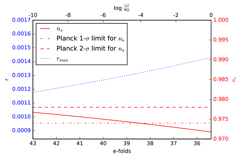
Figure 1: $n_{s}$ and $r_{\rm max}$ in hybrid inflation as a function of $\langle\phi\rangle$ and therefore $N$. The solid line depicts the values of $n_{s}$. The horizontal dashed lines correspond to the bounds from the 2015 Planck data on the spectral index (taken from Ref. [1]); the short-dashed line depicts the upper bound at 68% C.L. and the long-dashed line depicts the upper bound at 95% C.L.. The dotted line depicts the maximum allowed value for $r$, which corresponds to $\kappa=1$. Note that $n$ and $\lambda$ in Eq. (14) can both vary and hence the value of the VEV falls on a continuum.

$\langle\phi\rangle$	$N$	$n_{s}$	$r_{\rm max}$
$m_{P}$	35.4	0.972	1.4$\times 10^{-3}$
$10^{10}\,$GeV	41.5	0.976	1.2$\times 10^{-3}$

Table 2: $n_{s}$ and $r_{\rm max}$ in hybrid inflation, with minimum $N$ and $\kappa=1$ (for maximum $r$).

Fig. 1 clearly shows our range of values for $n_{s}$ inside the parameter space of the Planck results, at the 2-$\sigma$ level. For large values of the VEV; i.e. more than $10^{13}\,$GeV or so, $n_{s}$ enters inside the 1-$\sigma$ region. This corresponds to $n\geq 2$ in Eq. (14), which, in view of Eq. (15), suggests that the flaton mass is $\geq 2.4\,$TeV, which is safely above the latest LHC bounds.

5 Conclusions

In conclusion, we have demonstrated that late reheating followed by a subsequent period of thermal inflation can enable the minimal hybrid inflation in supergravity model to successfully produce cosmological perturbations with spectral index allowed by the Planck satellite observations. We have achieved this without affecting or modifying in the least the inflationary model, retaining thereby the accidental calcellation that resolves the $\eta$-problem of inflation in supergravity with minimal Kähler potential. Furthermore, we also found that the tensor to scalar ratio can be significantly increased such that it may become observable in the near future. It is important to stress that the above mechanism may also have profound implications for other inflationary models, see for example Ref. [12].

References

- [1] P. A. R. Ade et al. [Planck Collaboration], arXiv:1502.02114 [astro-ph.CO].
- [2] A. D. Linde, Phys. Lett. B 259 1991 38; Phys. Rev. D 49 (1994) 748.
- [3] A. D. Linde and A. Riotto, Phys. Rev. D 56 (1997) 1841; G. R. Dvali, G. Lazarides and Q. Shafi, Phys. Lett. B 424 (1998) 259.
- [4] C. Pallis and Q. Shafi, Phys. Lett. B 736 (2014) 261; R. Armillis, G. Lazarides and C. Pallis, Phys. Rev. D 89 (2014) no.6, 065032; M. U. Rehman, Q. Shafi and J. R. Wickman, Phys. Rev. D 83 (2011) 067304.
- [5] B. Garbrecht, C. Pallis and A. Pilaftsis, JHEP 0612 (2006) 038.
- [6] G. Lazarides and C. Panagiotakopoulos, Phys. Rev. D 92 (2015) no.12, 123502; G. Lazarides and A. Vamvasakis, Phys. Rev. D 76 (2007) 123514.
- [7] G. Lazarides, Lect. Notes Phys. 592 (2002) 351.
- [8] D. Lyth, E. Stewart, Phys. Rev. D 53 (1995) 1784
- [9] E. W. Kolb and M. S. Turner, Front. Phys. 69 (1990) 1.
- [10] M. Dine, L. Randall and S. D. Thomas, Nucl. Phys. B 458 (1996) 291; Phys. Rev. Lett. 75 (1995) 398.
- [11] D. H. Lyth and A. Riotto, Phys. Rept. 314 (1999) 1.
- [12] K. Dimopoulos and C. Owen, arXiv:1607.02469 [hep-ph].