Measurement-only verifiable blind quantum computing with quantum input verification

Abstract

Verifiable blind quantum computing is a secure delegated quantum computing where a client with a limited quantum technology delegates her quantum computing to a server who has a universal quantum computer. The client’s privacy is protected (blindness) and the correctness of the computation is verifiable by the client in spite of her limited quantum technology (verifiability). There are mainly two types of protocols for verifiable blind quantum computing: the protocol where the client has only to generate single-qubit states, and the protocol where the client needs only the ability of single-qubit measurements. The latter is called the measurement-only verifiable blind quantum computing. If the input of the client’s quantum computing is a quantum state whose classical efficient description is not known to the client, there was no way for the measurement-only client to verify the correctness of the input. Here we introduce a new protocol of measurement-only verifiable blind quantum computing where the correctness of the quantum input is also verifiable.

I Introduction

Blind quantum computing is a secure delegated quantum computing where a client (Alice) who does not have enough quantum technology delegates her quantum computing to a server (Bob) who has a universal quantum computer without leaking any information about her quantum computing. By using measurement-based quantum computing MBQC ; MBQC2 , Broadbent, Fitzsimons, and Kashefi first showed that blind quantum computing is indeed possible for a client who can do only the single qubit state generation BFK . Since the breakthrough, many theoretical improvements have been obtained MFNatComm ; CV ; coherent ; Lorenzo ; Mantri ; distillation ; composable ; AKLT ; Sueki , and even a proof-of-principle experiment was achieved with photonic qubits experiment1 . These blind quantum computing protocols guarantee two properties: first, if Bob is honest, Alice can obtain the correct result of her quantum computing (correctness). Second, whatever Bob does, he cannot gain any information about Alice’s quantum computing (blindness) unavoidable .

In stead of the single-qubit state generation, the ability of single-qubit measurements is also enough for Alice: it was shown in Ref. measuringAlice that Alice who can do only single-qubit measurements can perform blind quantum computing. The idea is that Bob generates a graph state and sends each qubit one by one to Alice. If Bob is honest, he generates the correct graph state and therefore Alice can perform the correct measurement-based quantum computing (correctness). If Bob is malicious, he might send a wrong state to Alice, but whatever Bob sends to Alice, Alice’s measurement angles, which contain information about Alice’s computation, cannot be transmitted to Bob due to the no-signaling principle (blindness). The protocol is called the measurement-only protocol, since Alice needs only measurements.

A problem in all these protocols is the lack of the verifiability: although the blindness guarantees that Bob cannot learn Alice’s quantum computing, he can still deviate from the correct procedure, mess up her quantum computing, and give Alice a completely wrong result. Since Alice cannot perform quantum computing by herself, she cannot check the correctness of the result by herself unless the problem is, say, in NP, and therefore she can accept a wrong result. To solve the problem, verifiable blind quantum computing protocol was introduced in Ref. FK , and some theoretical improvements were also obtained topoveri ; ElhamDI ; JoeDI . Experimental demonstrations of the verification were also done experiment2 ; experiment3 . The basic idea of these protocols is so called the trap technique: Alice hides some trap qubits in the register, and any change of a trap signals Bob’s malicious behavior. By checking traps, Alice can detect any Bob’s malicious behavior with high probability. If the computation is encoded by a quantum error detection code, the probability that Alice is fooled by Bob can be exponentially small, since in that case in order to change the logical state, Bob has to touch many qubits, and it consequently increases the probability that Bob touches some traps.

Recently, a new verification protocol that does not use the trap technique was proposed HM (see also Ref. HH ). In this protocol, Bob generates a graph state, and sends each qubit of it one by one to Alice. Alice directly verifies the correctness of the graph state (and therefore the correctness of the computation) sent from Bob by measuring stabilizer operators. This verification technique is called the stabilizer test. Note that the stabilizer test is useful also in quantum interactive proof system QMAsingle ; QAMsingle ; Matt ; FV ; Ji .

Although computing itself is verifiable through the stabilizer test, the input is not if it is a quantum state whose classical efficient description is not known to Alice. For example, let us assume that Alice receives a state $|\psi\rangle$ from Charlie, and she wants to apply a unitary $U$ on $|\psi\rangle$. If she delegates the quantum computation to Bob in the measurement-only style, a possible procedure is as follows. Alice first sends $|\psi\rangle$ to Bob. Bob next entangles $|\psi\rangle$ to the graph state. Bob then sends each qubit of the state one by one to Alice, and Alice does measurement-based quantum computing on it. If Bob is honest, Alice can realize $U|\psi\rangle$. Furthermore, as is shown in Refs. QMAsingle , Alice can verify the correctness of the graph state by using the stabilizer test even if some states are coupled to the graph state. However, in the procedure, the correctness of the input state is not guaranteed, since Bob does not necessarily couple $|\psi\rangle$ to the graph state, and Alice cannot check the correctness of the input state. Bob might discard $|\psi\rangle$ and entangles completely different state $|\psi^{\prime}\rangle$ to the graph state. In this case what Alice obtains is not $U|\psi\rangle$ but $U|\psi^{\prime}\rangle$. Can Alice verify that Bob honestly coupled her input state to the graph state?

In this paper, we introduce a new protocol of measurement-only verifiable blind quantum computing where not only the computation itself but also the quantum input are verifiable. Our strategy is to combine the trap technique and the stabilizer test. The correctness of the computing is verified by the stabilizer test, and the correctness of the quantum input is verified by checking the trap qubits that are randomly hidden in the input state. When the traps are checked, the state can be isolated from the graph state by measuring the connecting qubits in $Z$ basis. The main technical challenge in our proof is to show that the trap verification and the stabilizer verification can coexist with each other.

II Stabilizer test

We first review the stabilizer test. Let us consider an $N$-qubit state $\rho$ and a set $g\equiv\{g_{1},...,g_{n}\}$ of generators of a stabilizer group. The stabilizer test is a following test:

• Randomly generate an $n$-bit string $k\equiv(k_{1},...,k_{n})\in\{0,1\}^{n}$.

• Measure the operator

  $$s_{k}\equiv\prod_{j=1}^{n}g_{j}^{k_{j}}.$$

  Note that this measurement can be done with single-qubit measurements, since $s_{k}$ is a tensor product of Pauli operators.

• If the result is $+1$ ($-1$), the test passes (fails).

The probability of passing the stabilizer test is

$$p_{pass}=\frac{1}{2^{n}}\sum_{k\in\{0,1\}^{n}}\mbox{Tr}\Big{(}\frac{I+s_{k}}{2}\rho\Big{)}.$$

We can show that if the probability of passing the test is high, $p_{pass}\geq 1-\epsilon$, then $\rho$ is “close” to a certain stabilized state $\sigma$ in the sense of

$$\mbox{Tr}(M\sigma)(1-2\epsilon)-\sqrt{2\epsilon}\leq\mbox{Tr}(M\rho)\leq\mbox{Tr}(M\sigma)+\sqrt{2\epsilon}$$ (1)

for any POVM element $M$.

In fact, if $p_{pass}\geq 1-\epsilon$, we obtain

$$\mbox{Tr}\Big{(}\prod_{j=1}^{k}\frac{I+g_{j}}{2}\rho\Big{)}\geq 1-2\epsilon.$$

Let

$$\Lambda\equiv\prod_{j=1}^{k}\frac{I+g_{j}}{2}.$$

From the gentle measurement lemma gentle ,

$$\frac{1}{2}\|\rho-\Lambda\rho\Lambda\|_{1} \leq \sqrt{1-\mbox{Tr}(\Lambda\rho)}$$

$$\leq \sqrt{1-(1-2\epsilon)}$$

$$= \sqrt{2\epsilon}.$$

Note that

$$g_{j}\frac{\Lambda\rho\Lambda}{\mbox{Tr}(\Lambda\rho)}g_{j}=\frac{\Lambda\rho\Lambda}{\mbox{Tr}(\Lambda\rho)}$$

for any $j$, and therefore, $\Lambda\rho\Lambda/\mbox{Tr}(\Lambda\rho)$ is a stabilized state.

For any positive operator $M$,

$$\mbox{Tr}(M\rho)-\mbox{Tr}(\Lambda\rho\Lambda)\leq\sqrt{2\epsilon},$$

which means

$$\mbox{Tr}(M\rho) \leq \mbox{Tr}\Big{(}M\frac{\Lambda\rho\Lambda}{\mbox{Tr}(\Lambda\rho)}\Big{)}{\mbox{Tr}(\Lambda\rho)}+\sqrt{2\epsilon}$$

$$\leq \mbox{Tr}\Big{(}M\frac{\Lambda\rho\Lambda}{\mbox{Tr}(\Lambda\rho)}\Big{)}+\sqrt{2\epsilon}.$$

And, for any positive operator $M$,

$$\mbox{Tr}(\Lambda\rho\Lambda)-\mbox{Tr}(M\rho)\leq\sqrt{2\epsilon},$$

which means

$$\mbox{Tr}(M\rho) \geq \mbox{Tr}\Big{(}M\frac{\Lambda\rho\Lambda}{\mbox{Tr}(\Lambda\rho)}\Big{)}\mbox{Tr}(\Lambda\rho)-\sqrt{2\epsilon}$$

$$\geq \mbox{Tr}\Big{(}M\frac{\Lambda\rho\Lambda}{\mbox{Tr}(\Lambda\rho)}\Big{)}(1-2\epsilon)-\sqrt{2\epsilon}.$$

III Our protocol

Now we explain our protocol and analyze it, which is the main result of the present paper. Let us consider the following situation: Alice possesses an $m$-qubit state $|\psi\rangle$, but she neither knows its classical description nor a classical description of a quantum circuit that efficiently generates the state. (For example, she just receives $|\psi\rangle$ from her friend Charlie, etc.) She wants to perform a polynomial-size quantum computing $U$ on the input $|\psi\rangle$, but she cannot do it by herself. She therefore asks Bob, who is very powerful but not trusted, to perform her quantum computing. We show that Alice can delegate her quantum computing to Bob without revealing $|\psi\rangle$ and $U$, and she can verify the correctness of the computation and input.

For simplicity, we assume that Alice wants to solve a decision problem $L$. Alice measures the output qubit of $U|\psi\rangle$ in the computational basis, and accepts (rejects) if the result is 1 (0). As usual, we assume that for any yes instance $x$, i.e., $x\in L$, the acceptance probability is larger than $a$, and for any no instance $x$, i.e., $x\notin L$, the acceptance probability is smaller than $b$, where $a-b\geq 1/poly(|x|)$.

Our protocol runs as follows:

• Alice randomly chooses a $3m$-qubit permutation $P$, and applies it on

  $$|\Psi\rangle\equiv|\psi\rangle\otimes|0\rangle^{\otimes m}\otimes|+\rangle^{\otimes m}$$

  to generate $P|\Psi\rangle$. Alice further chooses a random $6m$-bit string $(x_{1},...,x_{3m},z_{1},...,z_{3m})\in\{0,1\}^{6m}$, and applies $\bigotimes_{j=1}^{3m}X_{j}^{x_{j}}Z_{j}^{z_{j}}$ on $P|\Psi\rangle$ to generate

  $$|\Psi^{\prime}\rangle\equiv\Big{(}\bigotimes_{j=1}^{3m}X_{j}^{x_{j}}Z_{j}^{z_{j}}\Big{)}P|\Psi\rangle.$$

  She sends $|\Psi^{\prime}\rangle$ to Bob. (Or, it is reasonable to assume that Charlie gives Alice $|\Psi^{\prime}\rangle$ and information of $P$ and $(x_{1},...,x_{3m},z_{1},...,z_{3m})$ in stead of giving $|\psi\rangle$.)

• If Bob is honest, he generates the $(3m+N)$-qubit state

  $$|G_{\Psi^{\prime}}\rangle\equiv\Big{(}\bigotimes_{e\in E_{connect}}CZ_{e}\Big{)}(|\Psi^{\prime}\rangle\otimes|G\rangle),$$ (2)

  and sends each qubit of it one by one to Alice, where $CZ_{e}$ is the CZ gate on the vertices of the edge $e$, and $E_{connect}$ is the set of edges that connects qubits in $|G\rangle$ and $|\Psi^{\prime}\rangle$ (Fig. 1). If Bob is malicious, he sends any $(3m+N)$-qubit state $\rho$ to Alice.

• • With probability $q$, which is specified later, Alice does the measurement-based quantum computing on qubits sent from Bob. If the computation result is accept (reject), she accepts (rejects). (During the computation, Alice of course corrects the initial random Pauli operator and permutation $(\bigotimes_{j=1}^{3m}X_{j}^{x_{j}}Z_{j}^{z_{j}})P$.)

  • With probability $(1-q)/2$, Alice does the stabilizer test, and if she passes (fails) the test, she accepts (rejects).

  • With probability $(1-q)/2$, Alice does the following test, which we call the input-state test: Let $V_{1}$ and $V_{2}$ be the set of qubits in the red dotted box and the blue dotted box in Fig. 1, respectively. Alice stores qubits in $V_{2}$ in her memory, and measures each qubit in $V_{1}$ in $Z$ basis. If the $Z$-basis measurement result on the nearest-neighbour of $j$th vertex in $V_{2}$ is 1, Alice applies $Z$ on the $j$th vertex in $V_{2}$ for $j=1,...,3m$. If Bob was honest, the state of $V_{2}$ is now

    $$|\Psi^{\prime}\rangle=\Big{(}\bigotimes_{j=1}^{3m}X_{j}^{x_{j}}Z_{j}^{z_{j}}\Big{)}P|\Psi\rangle.$$

    Alice further applies $P^{\dagger}(\bigotimes_{j=1}^{3m}X_{j}^{x_{j}}Z_{j}^{z_{j}})$ on $V_{2}$. If Bob was honest, the state of $V_{2}$ is now $|\Psi\rangle=|\psi\rangle\otimes|0\rangle^{\otimes m}\otimes|+\rangle^{\otimes m}$. Then Alice performs the projection measurement $\{\Lambda_{0}\equiv|0\rangle\langle 0|^{\otimes m}\otimes|+\rangle\langle+|^{\otimes m},\Lambda_{1}=I^{\otimes 2m}-\Lambda_{0}\}$, on the last $2m$ qubits of $V_{2}$. If she gets $\Lambda_{0}$, she accepts. Otherwise, she rejects.

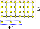
Figure 1: The state $|G_{\Psi^{\prime}}\rangle$. The state in the red dotted box is $|G\rangle$ and that in the blue dotted box is $|\Psi^{\prime}\rangle$. $E_{connect}$ is the set of edges that connects qubits in the red dotted box and those in the blue dotted box.

Now let us analyze the protocol. First, the blindness is obvious, since what she sends to Bob is the completely-mixed state from Bob’s view point, and due to the no-signaling principle, Alice’s operations on states sent from Bob do not transmit any information to Bob.

Second, let us consider the case of $x\in L$. In this case, honest Bob generates the correct state, $|G_{\Psi^{\prime}}\rangle$, Eq. (2), and therefore Alice can do correct computation, if she chooses the measurement-based quantum computing, passes the stabilizer test with probability 1, if she chooses the stabilizer test, and passes the input-state test with probability 1, if she chooses the input-state test. Therefore, the acceptance probability, $p_{acc}^{x\in L}$, is

$$p_{acc}^{x\in L} \geq qa+\frac{1-q}{2}\times 1+\frac{1-q}{2}\times 1$$

$$= qa+(1-q)\equiv\alpha.$$

Finally, let us consider the case of $x\notin L$. In this case, Bob might be malicious, and can send any $(3m+N)$-qubit state $\rho$. Let $p_{Gpass}$ and $p_{\psi pass}$ be the probability of passing the stabilizer test and the initial-state test, respectively.

Let $\epsilon=\frac{1}{poly(|x|)}$. It is easy to see that the acceptance probability, $p_{acc}^{x\notin L}$, is given as follows:

• If $p_{Gpass}\geq 1-\epsilon$ and $p_{\psi pass}<1-\epsilon$, then

  $$p_{acc}^{x\notin L} < q+\frac{1-q}{2}+\frac{1-q}{2}(1-\epsilon)\equiv\beta_{1}.$$

• If $p_{Gpass}<1-\epsilon$ and $p_{\psi pass}\geq 1-\epsilon$, then

  $$p_{acc}^{x\notin L} < q+\frac{1-q}{2}(1-\epsilon)+\frac{1-q}{2}=\beta_{1}.$$

• If $p_{Gpass}<1-\epsilon$ and $p_{\psi pass}<1-\epsilon$, then

  $$p_{acc}^{x\notin L} < q+\frac{1-q}{2}(1-\epsilon)+\frac{1-q}{2}(1-\epsilon)$$

  $$= q+(1-q)(1-\epsilon)\equiv\beta_{2}.$$

Let us consider the remaining case, $p_{Gpass}\geq 1-\epsilon$ and $p_{\psi pass}\geq 1-\epsilon$. From the triangle inequality and the invariance of the trace norm under a unitary operation, we obtain

$$\frac{1}{2}\big{\|}\rho-G_{\Psi^{\prime}}\big{\|}_{1} = \frac{1}{2}\big{\|}\rho-G_{\sigma}+G_{\sigma}-G_{\Psi^{\prime}}\big{\|}_{1}$$

$$\leq \frac{1}{2}\big{\|}\rho-G_{\sigma}\big{\|}_{1}+\frac{1}{2}\big{\|}G_{\sigma}-G_{\Psi^{\prime}}\big{\|}_{1}$$

$$= \frac{1}{2}\big{\|}\rho-G_{\sigma}\big{\|}_{1}+\frac{1}{2}\big{\|}\sigma-|\Psi^{\prime}\rangle\langle\Psi^{\prime}|\big{\|}_{1},$$

where $G_{\Psi^{\prime}}\equiv|G_{\Psi^{\prime}}\rangle\langle G_{\Psi^{\prime}}|$,

$$G_{\sigma}\equiv\big{(}\bigotimes_{e\in E_{connect}}CZ_{e}\big{)}(\sigma\otimes|G\rangle\langle G|)\big{(}\bigotimes_{e\in E_{connect}}CZ_{e}\big{)},$$

and $\sigma$ is any $3m$-qubit state on $V_{2}$. Since $p_{Gpass}\geq 1-\epsilon$, the first term is upperbounded as

$$\frac{1}{2}\big{\|}\rho-G_{\sigma}\big{\|}_{1}\leq\sqrt{2\epsilon},$$

from Eq. (1). We can show that if $p_{\psi pass}\geq 1-\epsilon$, the second term is upperbounded as

$$\frac{1}{2}\big{\|}\sigma-|\Psi^{\prime}\rangle\langle\Psi^{\prime}|\big{\|}_{1}\leq\sqrt{2\epsilon}+\sqrt{\frac{2}{3}+\epsilon}.$$ (3)

The proof is given in Appendix.

Therefore, we obtain

$$\frac{1}{2}\big{\|}\rho-G_{\Psi^{\prime}}\big{\|}_{1} \leq 2\sqrt{2\epsilon}+\sqrt{\frac{2}{3}+\epsilon}$$

$$\equiv \delta,$$

which means

$$\big{|}\mbox{Tr}(\Pi\rho)-\mbox{Tr}(\Pi G_{\Psi^{\prime}})\big{|}\leq\delta$$

for the POVM element $\Pi$ corresponding to the acceptance of the measurement-based quantum computing. Therefore, the total acceptance probability, $p_{acc}^{x\notin L}$, is

$$p_{acc}^{x\notin L} \leq q(b+\delta)+\frac{1-q}{2}+\frac{1-q}{2}$$

$$= q(b+\delta)+(1-q)\equiv\beta_{3}.$$

Let us define

$$\Delta_{1}(q) \equiv \alpha-\beta_{1}=q(a-1)+\frac{\epsilon(1-q)}{2},$$

$$\Delta_{2}(q) \equiv \alpha-\beta_{2}=q(a-1)+\epsilon(1-q),$$

$$\Delta_{3}(q) \equiv \alpha-\beta_{3}=q(a-b-\delta).$$

The optimal value

$$q^{*}\equiv\frac{\frac{\epsilon}{2}}{1+\frac{\epsilon}{2}-b-\delta}$$

of $q$ is that satisfies $\Delta_{1}(q)=\Delta_{3}(q)$. Then, if we take $a=1-2^{-r}$ and $b=2^{-r}$ for a polynomial $r$,

$$\Delta_{3}(q^{*}) = \frac{\frac{\epsilon}{2}(a-b-\delta)}{1+\frac{\epsilon}{2}-b-\delta}$$

$$\geq \frac{\epsilon}{4}\Big{(}1-2^{-r+1}-2\sqrt{2\epsilon}-\sqrt{\frac{2}{3}+\epsilon}\Big{)}$$

$$\geq \frac{1}{poly(|x|)}.$$

As usual, the inverse polynomial gap can be amplified with a polynomial overhead.

*

Appendix A Proof of Eq. (3)

In this appendix, we show Eq. (3). Due to the triangle inequality and the invariance of the trace norm under a unitary operation,

$$\frac{1}{2}\big{\|}\sigma-|\Psi^{\prime}\rangle\langle\Psi^{\prime}|\big{\|}_{1} = \frac{1}{2}\Big{\|}\sigma-\big{(}\bigotimes_{j=1}^{3m}X_{j}^{x_{j}}Z_{j}^{z_{j}}\big{)}P\big{(}\framebox{$\psi$}\otimes\framebox{0}^{\otimes m}\otimes\framebox{+}^{\otimes m}\big{)}P^{\dagger}\big{(}\bigotimes_{j=1}^{3m}X_{j}^{x_{j}}Z_{j}^{z_{j}}\big{)}\Big{\|}_{1}$$

$$= \frac{1}{2}\Big{\|}P^{\dagger}\big{(}\bigotimes_{j=1}^{3m}X_{j}^{x_{j}}Z_{j}^{z_{j}}\big{)}\sigma\big{(}\bigotimes_{j=1}^{3m}X_{j}^{x_{j}}Z_{j}^{z_{j}}\big{)}P-\framebox{$\psi$}\otimes\framebox{0}^{\otimes m}\otimes\framebox{+}^{\otimes m}\Big{\|}_{1}$$

$$\leq \frac{1}{2}\Big{\|}P^{\dagger}\big{(}\bigotimes_{j=1}^{3m}X_{j}^{x_{j}}Z_{j}^{z_{j}}\big{)}\sigma\big{(}\bigotimes_{j=1}^{3m}X_{j}^{x_{j}}Z_{j}^{z_{j}}\big{)}P-\rho_{before}\Big{\|}_{1}$$

$$+\frac{1}{2}\Big{\|}\rho_{before}-\framebox{$\psi$}\otimes\framebox{0}^{\otimes m}\otimes\framebox{+}^{\otimes m}\Big{\|}_{1},$$

where $\rho_{before}$ is the state before measuring $\{\Lambda_{0},\Lambda_{1}\}$.

From the monotonicity of the trace distance under a CPTP map, the first term is upperbounded as

$$\frac{1}{2}\Big{\|}P^{\dagger}\big{(}\bigotimes_{j=1}^{3m}X_{j}^{x_{j}}Z_{j}^{z_{j}}\big{)}\sigma\big{(}\bigotimes_{j=1}^{3m}X_{j}^{x_{j}}Z_{j}^{z_{j}}\big{)}P-\rho_{before}\Big{\|}_{1}\leq\frac{1}{2}\|G_{\sigma}-\rho\|_{1}\leq\sqrt{2\epsilon}.$$

As is shown below, the second term is upperbounded as

$$\frac{1}{2}\Big{\|}~{}\framebox{$\psi$}\otimes\framebox{0}^{\otimes m}\otimes\framebox{+}^{\otimes m}-\rho_{before}\Big{\|}_{1} \leq \sqrt{\frac{2}{3}+\epsilon}.$$ (4)

Therefore, we have shown Eq. (3).

Let us show Eq. (4). Note that

$$\rho_{before}=\frac{1}{(3m)!}\frac{1}{4^{3m}}\sum_{P,\alpha,k}P^{\dagger}\sigma_{\alpha}E_{k}\sigma_{\alpha}P\big{(}\framebox{$\psi$}\otimes\framebox{0}^{\otimes m}\otimes\framebox{+}^{\otimes m}\big{)}P^{\dagger}\sigma_{\alpha}E_{k}^{\dagger}\sigma_{\alpha}P,$$

where $\sigma_{\alpha}$ is a $3m$-qubit Pauli operator, and $E_{k}$ is a Kraus operator. Let us decompose each Kraus operator in terms of Pauli operators as $E_{k}=\sum_{\beta}C_{\beta}^{k}\sigma_{\beta}$. Since

$$I = \sum_{k}E_{k}^{\dagger}E_{k}$$

$$= \sum_{k,\beta,\gamma}C_{\beta}^{k*}C_{\gamma}^{k}\sigma_{\beta}\sigma_{\gamma}$$

$$= \sum_{k,\beta}|C_{\beta}^{k}|^{2}I+\sum_{k,\beta\neq\gamma}C_{\beta}^{k*}C_{\gamma}^{k}\sigma_{\beta}\sigma_{\gamma},$$

we obtain

$$\sum_{k,\beta}|C_{\beta}^{k}|^{2}=1.$$

Then,

$$\rho_{before} = \frac{1}{(3m)!}\frac{1}{4^{3m}}\sum_{P,\alpha,k,\beta,\gamma}C_{\beta}^{k}C_{\gamma}^{k*}P^{\dagger}\sigma_{\alpha}\sigma_{\beta}\sigma_{\alpha}P\big{(}\framebox{$\psi$}\otimes\framebox{0}^{\otimes m}\otimes\framebox{+}^{\otimes m}\big{)}P^{\dagger}\sigma_{\alpha}\sigma_{\gamma}\sigma_{\alpha}P$$

$$= \frac{1}{(3m)!}\sum_{P,k,\beta}|C_{\beta}^{k}|^{2}P^{\dagger}\sigma_{\beta}P\big{(}\framebox{$\psi$}\otimes\framebox{0}^{\otimes m}\otimes\framebox{+}^{\otimes m}\big{)}P^{\dagger}\sigma_{\beta}P$$

$$= \frac{1}{(3m)!}\sum_{P,\beta}D_{\beta}P^{\dagger}\sigma_{\beta}P\big{(}\framebox{$\psi$}\otimes\framebox{0}^{\otimes m}\otimes\framebox{+}^{\otimes m}\big{)}P^{\dagger}\sigma_{\beta}P$$

$$= D_{0}\big{(}\framebox{$\psi$}\otimes\framebox{0}^{\otimes m}\otimes\framebox{+}^{\otimes m}\big{)}+\frac{1}{(3m)!}\sum_{P,\beta\neq 0}D_{\beta}P^{\dagger}\sigma_{\beta}P\big{(}\framebox{$\psi$}\otimes\framebox{0}^{\otimes m}\otimes\framebox{+}^{\otimes m}\big{)}P^{\dagger}\sigma_{\beta}P$$

$$\equiv \rho_{1}+\rho_{2}.$$

Here, $\sigma_{0}=I^{\otimes 3m}$, we have used the relation

$$\sum_{\alpha}\sigma_{\alpha}\sigma_{\beta}\sigma_{\alpha}\rho\sigma_{\alpha}\sigma_{\gamma}\sigma_{\alpha}=0$$

for any $\rho$ and $\beta\neq\gamma$, and defined

$$\sum_{k}|C_{\beta}^{k}|^{2}=D_{\beta}.$$

Note that

$$\sum_{\beta}D_{\beta}=\sum_{\beta,k}|C_{\beta}^{k}|^{2}=1.$$

It is obvious that

$$\mbox{Tr}\Big{[}\big{(}I^{\otimes m}-\framebox{$\psi$}\big{)}\otimes\framebox{0}^{\otimes m}\otimes\framebox{+}^{\otimes m}\times\rho_{1}\Big{]}=0.$$

Furthermore,

$$\mbox{Tr}\Big{[}\big{(}I^{\otimes m}-\framebox{$\psi$}\big{)}\otimes\framebox{0}^{\otimes m}\otimes\framebox{+}^{\otimes m}\times\rho_{2}\Big{]}$$

$$= \frac{1}{(3m)!}\sum_{P,\beta\neq 0}D_{\beta}\mbox{Tr}\Big{[}\big{(}I^{\otimes m}-\framebox{$\psi$}\big{)}\otimes\framebox{0}^{\otimes m}\otimes\framebox{+}^{\otimes m}\times P^{\dagger}\sigma_{\beta}P\big{(}\framebox{$\psi$}\otimes\framebox{0}^{\otimes m}\otimes\framebox{+}^{\otimes m}\big{)}P^{\dagger}\sigma_{\beta}P\Big{]}$$

$$\leq \frac{1}{(3m)!}\sum_{\beta\neq 0}D_{\beta}(2m\times(3m-1)!)$$

$$\leq \frac{2m\times(3m-1)!}{(3m)!}$$

$$= \frac{2}{3}.$$

Therefore,

$$\mbox{Tr}\Big{[}\big{(}I^{\otimes m}-\framebox{$\psi$}\big{)}\otimes\framebox{0}^{\otimes m}\otimes\framebox{+}^{\otimes m}\times\rho_{before}\Big{]}\leq\frac{2}{3},$$

which means

$$\mbox{Tr}\Big{[}\framebox{$\psi$}\otimes\framebox{0}^{\otimes m}\otimes\framebox{+}^{\otimes m}\times\rho_{before}\Big{]} \geq \mbox{Tr}\Big{[}I^{\otimes m}\otimes\framebox{0}^{\otimes m}\otimes\framebox{+}^{\otimes m}\times\rho_{before}\Big{]}-\frac{2}{3}$$

$$\geq 1-\epsilon-\frac{2}{3}$$

$$= \frac{1}{3}-\epsilon,$$

where we have used the assumption that

$$p_{\psi pass}=\mbox{Tr}\Big{[}I^{\otimes m}\otimes\framebox{0}^{\otimes m}\otimes\framebox{+}^{\otimes m}\times\rho_{before}\Big{]}\geq 1-\epsilon.$$

Therefore

$$\frac{1}{2}\Big{\|}~{}\framebox{$\psi$}\otimes\framebox{0}^{\otimes m}\otimes\framebox{+}^{\otimes m}-\rho_{before}\Big{\|}_{1} \leq \sqrt{1-\Big{(}\frac{1}{3}-\epsilon\Big{)}}$$

$$= \sqrt{\frac{2}{3}+\epsilon}.$$

References

(1)
R. Raussendorf and H. J. Briegel,
A one-way quantum computer.
Phys. Rev. Lett. 86, 5188 (2001).
(2)
R. Raussendorf, D. E. Browne, and H. J. Briegel,
Measurement-based quantum computation on cluster states.
Phys. Rev. A 68, 022312 (2003).
(3)
A. Broadbent, J. F. Fitzsimons, and E. Kashefi,
Universal blind quantum computation.
50th Annual IEEE Symposium on Foundations of Computer Science
(2009).
(4)
T. Morimae and K. Fujii,
Blind topological measurement-based quantum computation.
Nat. Comm. 3, 1036 (2012).
(5)
T. Morimae,
Continuous-variable blind quantum computation.
Phys. Rev. Lett. 109, 230502 (2012).
(6)
V. Dunjko, E. Kashefi, and A. Leverrier,
Universal blind quantum computing with weak coherent pulses.
Phys. Rev. Lett. 108, 200502 (2012).
(7)
V. Giovannetti, L. Maccone, T. Morimae, and T. G. Rudolph,
Efficient universal blind quantum computation.
Phys. Rev. Lett. 111, 230501 (2013).
(8)
A. Mantri, C. A. Perez-Delgado, and J. F. Fitzsimons,
Optimal blind quantum computation.
Phys. Rev. Lett. 111, 230502 (2013).
(9)
T. Morimae and K. Fujii,
Secure entanglement distillation for double-server blind quantum computation.
Phys. Rev. Lett. 111, 020502 (2013).
(10)
V. Dunjko, J. F. Fitzsimons, C. Portmann, and R. Renner,
Composable security of delegated quantum computation.
ASIACRYPT 2014, LNCS Volume 8874, pp406-425 (2014).
(11)
T. Morimae, V. Dunjko, and E. Kashefi,
Ground state blind quantum computation on AKLT state.
Quant. Inf. Comput. 15, 0200 (2015).
(12)
T. Sueki, T. Koshiba, and T. Morimae,
Ancilla-driven universal blind quantum computation.
Phys. Rev. A 87, 060301(R) (2013).
(13)
S. Barz, E. Kashefi, A. Broadbent, J. F. Fitzsimons,
A. Zeilinger, and P. Walther,
Experimental demonstration of blind quantum computing.
Science 335, 303 (2012).
(14)
Of course, some unavoidable leakage of information, such as the upperbound
of the computation size, occurs.
(15)
T. Morimae and K. Fujii,
Blind quantum computation protocol in which Alice only makes
measurements.
Phys. Rev. A 87, 050301(R) (2013).
(16)
J. F. Fitzsimons and E. Kashefi,
Unconditionally verifiable blind computation.
arXiv:1203.5217
(17)
T. Morimae,
Verification for measurement-only blind quantum computing.
Phys. Rev. A 89, 060302(R) (2014).
(18)
A. Gheorghiu, E. Kashefi, and P. Wallden,
Robustness and device independence of verifiable blind quantum
computing.
New J. Phys. 17, 083040 (2015).
(19)
M. Hajdusek, C. A. Perez-Delgado, and J. F. Fitzsimons,
Device-independent verifiable blind quantum computation.
arXiv:1502.02563
(20)
S. Barz, J. F. Fitzsimons, E. Kashefi, and P. Walther,
Experimental verification of quantum computations.
Nat. Phys. 9, 727 (2013).
(21)
C. Greganti, M. C. Roehsner, S. Barz, T. Morimae, and P. Walther,
Demonstration of measurement-only blind quantum computing.
New J. Phys. 18, 013020 (2016).
(22)
M. Hayashi and T. Morimae,
Verifiable measurement-only blind quantum computing
with stabilizer testing.
Phys. Rev. Lett. 115, 220502 (2015).
(23)
M. Hayashi and M. Hajdusek,
Self-guaranteed measurement-based quantum computation.
arXiv:1603.02195
(24)
T. Morimae, D. Nagaj, and N. Schuch,
Quantum proofs can be verified using only single qubit measurements.
Phys. Rev. A 93, 022326 (2016).
(25)
T. Morimae,
Quantum Arthur-Merlin with single-qubit measurements.
to appear in Phys. Rev. A.
(26)
M. McKague,
Interactive proofs for BQP via self-tested graph states.
arXiv:1309.5675
(27)
Z. Ji, Classical verification of quantum proofs.
arXiv:1505.07432
(28)
J. F. Fitzsimons and T. Vidick,
A multiprover interactive proof system for the local Hamiltonian problem.
arXiv:1409.0260
(29)
A. Winter,
Coding Theorem and Strong Converse for Quantum Channels.
IEEE Trans. Inf. Theory, vol. 45, no. 7, pp.2481-2485 (1999).