Three-particle correlation from a Many-Body Perspective:
Trions in a Carbon Nanotube

Abstract

Trion states of three correlated particles (e.g., two electrons and one hole) are essential to understand the optical spectra of doped or gated nanostructures, like carbon nanotubes or transition-metal dichalcogenides. We develop a theoretical many-body description for such correlated states using an ab-initio approach. It can be regarded as an extension of the widely used $GW$ method and Bethe-Salpeter equation, thus allowing for a direct comparison with excitons. We apply this method to a semiconducting (8,0) carbon nanotube, and find that the lowest optically active trions are red-shifted by $\sim 130$ meV compared to the excitons, confirming experimental findings for similar tubes. Moreover, our method provides detailed insights in the physical nature of trion states. In the prototypical carbon nanotube we find a variety of different excitations, discuss the spectra, energy compositions, and correlated wave functions.

Trions or “charged excitons” compete with excitons in the luminescence of carbon nanotubes (CNTs) Matsunaga et al. (2011); Santos et al. (2011); Park et al. (2012); Jakubka et al. (2014); Rønnow et al. (2009, 2010); Watanabe and Asano (2012); Nishihara et al. (2013); Yuma et al. (2013); Mouri et al. (2013a); Koyama et al. (2013) and transition-metal dichalcogenides Mak et al. (2013); Ross et al. (2013); Mouri et al. (2013b); Berkelbach et al. (2013). They result from correlation between (light-activated) excitons and additional charges (from doping or gating). However, detailed theoretical information about trions in atom-scaled systems, like CNTs, is very difficult to achieve for conceptual and numerical reasons. Here we develop an ab-initio many-body method that can describe trions on top of the widely used $GW$ method and Bethe-Salpeter equation (BSE). Our approach can thus be considered as an extension of the many-body perturbation theory (MBPT) Rohlfing and Louie (2000); Onida et al. (2002) to the situation of three correlated quasi-particles.

Trions are composed from electrons and holes forming correlated three-particle states in a condensed-matter system. In this work, we concentrate on two electrons and one hole (the treatment of a trion formed by two holes and one electron would be analogous and we expect similar results Park et al. (2012)). Usually one electron and one hole result from interband excitation by light, like an exciton in a charge-neutral system, while the third particle stems from impurities, intentional doping, or can be induced by a gate voltage. The actual source of the additional electron (doping, field effects, etc.) is not considered for our present description of trions. A trion state of two electrons and one hole with a total momentum K can be described as a linear combination of products of single-particle wave functions $\phi_{n{\bf k}}(x)$,

$$\Phi^{(T,{\bf K})} (x_{h},x_{1},x_{2})=\sum_{{\bf v},{\bf c}_{1},{\bf c}_{2}}A^{(T,{\bf K})}_{{\bf v},{\bf c}_{1},{\bf c}_{2}}\phi^{\ast}_{{\bf v}}(x_{h})\times$$

$$\times\frac{1}{\sqrt{2}}\left\{\phi_{{\bf c}_{1}}(x_{1})\phi_{{\bf c}_{2}}(x_{2})-\phi_{{\bf c}_{2}}(x_{1})\phi_{{\bf c}_{1}}(x_{2})\right\}$$ (1)

with ${\bf v}=(v,{\bf k}_{v})$ denoting band index and wave number of a hole in the valence bands (analogously, ${\bf c}_{1}$ and ${\bf c}_{2}$ for the two electrons in the conduction bands) and $x_{h}$, $x_{1}$, $x_{2}$ denoting their coordinates (position and spin). Due to Bloch’s theorem, the total momentum K is a good quantum number, and only wave vectors (from the first Brillouin zone) with ${\bf k}_{1}+{\bf k}_{2}-{\bf k}_{v}={\bf K}$ contribute to the sum. The trion states described within our framework (determined by the coefficients $A^{(T,{\bf K})}_{{\bf v},{\bf c}_{1},{\bf c}_{2}}$) are eigenstates of an effective Hamiltonian with matrix elements

$$\langle{\bf v}{\bf c}_{1}{\bf c}_{2}|\hat{H}^{(eeh)} |{\bf v}^{\prime}{\bf c}^{\prime}_{1}{\bf c}^{\prime}_{2}\rangle=$$ (2)

$$(\epsilon_{{\bf c}_{1}}+\epsilon_{{\bf c}_{2}}-\epsilon_{\bf v})\delta_{{\bf c}_{1},{\bf c}_{1}^{\prime}}\delta_{{\bf c}_{2},{\bf c}_{2}^{\prime}}\delta_{{\bf v},{\bf v}^{\prime}} (\hat{H}_{\text{BS}})\quad$$

$$+ (W_{{\bf c}_{1}{\bf c}_{2},{\bf c}^{\prime}_{1}{\bf c}^{\prime}_{2}}-W_{{\bf c}_{1}{\bf c}_{2},{\bf c}^{\prime}_{2}{\bf c}^{\prime}_{1}})\delta_{{\bf v},{\bf v}^{\prime}} (\hat{H}_{ee})\quad$$

$$- (W_{{\bf v}^{\prime}{\bf c}_{1},{\bf v}{\bf c}^{\prime}_{1}}-V_{{\bf v}^{\prime}{\bf c}_{1},{\bf c}^{\prime}_{1}{\bf v}})\delta_{{\bf c}_{2},{\bf c}_{2}^{\prime}} (\hat{H}_{eh,1})\quad$$

$$- (W_{{\bf v}^{\prime}{\bf c}_{2},{\bf v}{\bf c}^{\prime}_{2}}-V_{{\bf v}^{\prime}{\bf c}_{2},{\bf c}^{\prime}_{2}{\bf v}})\delta_{{\bf c}_{1},{\bf c}_{1}^{\prime}}~{}. (\hat{H}_{eh,2})\quad$$

Here, $\epsilon_{{\bf c}_{1}}\equiv\epsilon_{c_{1},{\bf k}_{1}}$ etc. denote the band-structure energies of a preceding $GW$ calculation. The first line of Eq. (2) describes the single particle contributions given by the system’s band structure, while the other terms describe the interaction (direct and exchange) between the two electrons, and between the hole and each of the electrons. Without the second electron Eq. (2) is reduced to $\langle{\bf v}{\bf c}|\hat{H}^{(eh)}|{\bf v}^{\prime}{\bf c}^{\prime}\rangle=(\epsilon_{\bf c}-\epsilon_{\bf v})\delta_{{\bf c}{\bf c}^{\prime}}\delta_{{\bf v}{\bf v}^{\prime}}-(W_{{\bf v}^{\prime}{\bf c},{\bf v}{\bf c}^{\prime}}-V_{{\bf v}^{\prime}{\bf c},{\bf c}^{\prime}{\bf v}})$, which are the matrix elements of the BSE Hamiltonian commonly used for excitons within MBPT Strinati (1982, 1984). Eq. (2) can be regarded as an extension of the BSE from two to three particles, allowing to directly compare the spectra of trions (from Eq. (2)) and excitons (from the BSE) in a consistent way. In semiconductor quantum systems, similar Hamiltonians are commonly employed Esser et al. (2000); Filinov et al. (2004); Narvaez et al. (2005); Rabani and Baer (2008); Huneke et al. (2011); Machnikowski and Kuhn (2011) (see next paragraph). A detailed discussion can be found in the Supplementary Material Note (1).

The general ab-initio determination of the Hamiltonian (2) constitutes a key issue of our study. In semiconductor quantum dots and similar structures, in which the relevant length scales are much larger than interatomic distances, $\hat{H}^{(eeh)}$ may be constructed from empirical parameters (e.g., effective masses, one single dielectric-constant value, etc.) Esser et al. (2000); Filinov et al. (2004); Narvaez et al. (2005); Rabani and Baer (2008); Huneke et al. (2011); Machnikowski and Kuhn (2011). In a CNT, on the other hand, excitonic binding occurs on a much smaller length scale of about one nanometer. Inter-atomic electronic-structure details become important, and dielectric screening properties are inhomogeneous and anisotropic on such small length scale. A priori, it is not clear if a parameter-controlled modelling of $\hat{H}^{(eeh)}$ Esser et al. (2000); Filinov et al. (2004); Narvaez et al. (2005); Rabani and Baer (2008); Huneke et al. (2011); Machnikowski and Kuhn (2011) is sufficient. To overcome system specific modelling, we perform a general determination of $\hat{H}^{(eeh)}$ for one-, two-, and three-dimensional systems (and gain full access to the atomic composition). This must be performed on a microscopic level, including many-body effects, starting from atom- and orbital-resolved single-particle wave functions $\phi_{n{\bf k}}(x)$. Thereby the six-dimensional dielectric function $\epsilon({\bf r},{\bf r}^{\prime})$ evaluated from $\phi_{n{\bf k}}(x)$ and their energies $\epsilon_{n{\bf k}}$ within the random-phase approximation is also included [rather than using a dielectric constant $\epsilon$ or a simple distance dependence $\epsilon(|{\bf r}-{\bf r}^{\prime}|)$]. The dielectric function is needed for the screened Coulomb interaction ($W({\bf r},{\bf r}^{\prime})=\int\epsilon^{-1}({\bf r},{\bf r}^{\prime\prime})V({\bf r}^{\prime\prime},{\bf r}^{\prime})d^{3}r^{\prime\prime}$) which contains the full information about spatial inhomogeneity and anisotropy. Such procedure was the key to understand excitons in CNTs Spataru et al. (2004); Chang et al. (2004); Mu et al. (2013); Rohlfing (2012) within an ab-initio $GW$/BSE approach. We note that (in contrast to many model Hamiltonians) the screened interaction ($W_{{\bf c}_{1}{\bf c}_{2},{\bf c}_{1}^{\prime}{\bf c}_{2}^{\prime}}$ etc.) within $GW$/BSE (see e.g. Johnson and Hulbert (1987); Puschnig et al. (2012); Milko et al. (2012, 2013); Neaton et al. (2006); Garcia-Lastra et al. (2009); Garcia-Lastra and Thygesen (2011); Rohlfing (2012)) acts in a natural way on the band structure ($\epsilon_{\bf{v}}$ etc.), on the excitonic binding, and on the trions on equal footing. We also note that polaronic or self-trapping effects, localized charges at defects/dopant atoms, as well as high-density effects (bleaching, band-gap renormalization etc.) are not considered within our framework.

In contract to excitons (described by the BSE), the configurational space of trions is much larger, which prohibits the standard diagonalization of the Hamiltonian of Eq. (2). For instance, our typical calculations for the (8,0) nanotube include 16 valence bands, 16 conduction bands, and 32 $\bf k$-points, yielding a trion configuration space of $\sim\frac{1}{2}16^{3}\times 32^{2}$ $\sim$ $2.1\times 10^{6}$ (as compared to an exciton configuration space of only $16^{2}\times 32$ = 8192). The unit cell contains $32$ atoms (Fig. S1 of the Supplementary Material), for the evaluation of excitons and trions this cell is extended by a factor of 32 (due to the usage of 32 $\bf k$-points). This extended unit cell is shown in Fig. 3. Fortunately, all Coulomb interaction terms (bare or screened, direct or exchange) in Eq. (2) are of two-particle nature only, and the resulting Hamilton matrix is very sparse Note (1). This opens an avenue to deal with the trion Hamiltonian iteratively, either by Haydock recursion or similar Haydock et al. (1972); Schmidt et al. (2003) when focusing on spectra, or by the Lanczos algorithm or similar Hernandez et al. (2005) when eigenstates are requested. Such an iterative procedure, together with parallel architecture make our approach feasible .

Having set up a general method to describe trions, we are now able to discuss trions in a prototypical low-dimensional system on the atomic scale, i.e. the (8,0) CNT. Figure 1 shows our calculated absorption spectra of excitons and trions (upper panel) and corresponding room-temperature luminescence spectra (lower panel). We want to stress that in most common experimental set-ups the spectra show the combined effects of trions and excitons.

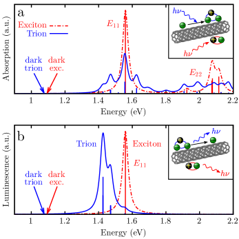
Figure 1: Optical absorption and luminescence spectrum of an (8,0) carbon nanotube. (a) Optical absorption due to excitons (red dashed lines) and due to negatively charge trions (blue lines). The arrows at $1.09$ eV (exciton) and at $1.07$ eV (trion) indicate the onset of the spectrum, which is not visible because of zero optical dipole strength of the corresponding states. (b) Luminescence spectrum from the $E_{11}$ exciton and from the related optically allowed trions, assuming that the occupancy of the excited states relative to each other is given by a Boltzmann distribution at room temperature (see Supplementary Material). This distribution highlights the lower-energy states near $1.4$ eV and suppresses states above $1.5$ eV. In all cases the electric-field vector of the light is along the tube axis. Note that the amplitudes of the exciton and trion spectrum cannot be compared with one another because the trion spectrum scales with the density of donated electrons. The trions have been calculated for ${\bf K}=0$, at which the optical dipoles are by far the strongest. We consider transitions to the conduction-band minimum. Including non-zero K yields very similar results. An artificial broadening of $0.02$ eV is used.

The exciton spectrum exhibits two distinct peaks ($E_{11}$ and $E_{22}$), but there are also many dark excitons (triplet excitons and dipole-forbidden singlet excitons), starting at an onset of $1.09$ eV . These excitons are accompanied by a variety of trion states. At the low-energy onset, the first trion state is found at $1.07$ eV. The first dipole-allowed trion, however, is found slightly below the $E_{11}$ exciton, at $1.43$ eV, together with several other dipole-allowed trions below and above the $E_{11}$ exciton. More states are observed at and above $1.8$ eV. A more drastic picture emerges in the luminescence spectrum, which contains the same excitations, but with weights that simulate a luminescence experiment Note (1, 4). Here we simply assume that the trions (and excitons as well) achieve thermal equilibrium after the excitation process, with energy dependent occupation probabilities given by a room-temperature Boltzmann distribution (see Supplementary Material). Luminescence from trions then occurs predominantly from those states near $1.4$ eV, i.e. $\sim$130 meV below the $E_{11}$ exciton, which dominates the exciton luminescence .

Experimental spectra similar to Fig. 1 have been measured for various CNTs, with red-shifts of 100-200 meV Matsunaga et al. (2011); Park et al. (2012); Jakubka et al. (2014) between trion and exciton luminescence. Unfortunately, we are not aware of any trion experiment on an (8,0) CNT yet, and most CNTs from experiment have more complicated chirality and are thus numerically too demanding for our present study. However, our results show redshifts of the same size. We note that the trionic binding effects between exciton and electron strongly differ from state to state. For example, the dark states near $1.1$ eV exhibit a much smaller redshift of only $\sim$20 meV.

Table 1: Energy composition of the exciton and trion energies. Transition energy $\Omega$, band-structure term $\langle E_{\text{BS}}\rangle$, electron-hole interaction $\langle E_{eh}\rangle$, and electron-electron interaction $\langle E_{ee}\rangle$ for the lowest dark and bright states (in eV), for zero total momentum (exciton: ${\bf Q}=0$, trion: ${\bf K}=0$). For further details see main text.

(eV)	$\Omega$	$\langle E_{\text{BS}}\rangle$	$\langle E_{eh}\rangle$	$\langle E_{ee}\rangle$
dark exciton	$1.09$	$2.17$	$-1.08$	–
dark trion	$1.07$	$2.18$	$-1.65$	$0.56$
bright exciton	$1.56$	$2.51$	$-0.95$	–
bright trion	$1.43$	$2.60$	$-1.69$	$0.52$

We now discuss the energetics of the trions in comparison to excitons (Tab. 1). For an exciton, $\Omega$ is the eigenvalue of the corresponding Hamiltonian. For a trion, $\Omega$ is given as the difference between the eigenvalue of the Hamiltonian (2) and the CBM energy (see Supplementary Material), which allows a systematic comparison. $\Omega$ thus immediately gives the transition energy for the transition from the trion to the electron remaining in the CBM at zero momentum (i.e., at the $\Gamma$ point). For the trions, $\langle E_{\text{BS}}\rangle$ is also given relative to the CBM. This band is chosen because the (radiative) decay of a trion (with ${\bf K}=0$) is mostly into the CBM, so the calibration to the CBM immediately yields the luminescence frequency of the transition (cf. Fig. 1). All other values are expectation values of the corresponding terms to the Hamiltonians $\langle E_{i}\rangle=\langle\Phi|\hat{H}_{i}|\Phi\rangle$, with $\Phi$ denoting the wave function.
Both for excitons and for trions we discuss in Tab. 1 the lowest-energy states (which happen to have zero dipole moment, i.e. these are dark states) and the first bright states. The compositions of the bright states from bands and wave numbers is also shown in Fig. 2. Both dark states and both bright states show about the same band-structure contribution, $\langle E_{\text{BS}}\rangle$, indicating similar composition from the bands. The bright exciton, e.g., is composed from the highest valence band and from the CBM+3 conduction band (excitons from lower conduction bands are dark, or involve deeper valence electrons which leads to higher transition energies). The bright trion similarly involves one electron in the CBM+3 band (see Fig. 2) while the other electron is mostly located in the CBM band. The main difference between excitons and trions is in the Coulomb interaction. The trions observe electron-electron repulsion $\langle E_{ee}\rangle$ which is of course absent in the excitons. They also observe stronger electron-hole attraction because there are two electrons to which the hole is attracted. However, $\langle E_{eh}\rangle$ is less than twice as strong compared to the exciton, because the electron-electron repulsion drives the electrons somewhat apart from each other, thus weakening the attraction of both of them to the hole.

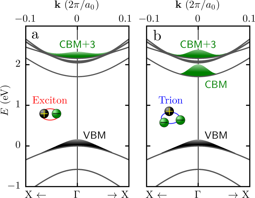
Figure 2: Band structure of an (8,0) CNT, showing the composition of the lowest bright exciton (a) and trion (b). The black bell-shaped distributions on the highest valence band indicate the composition of the hole as a function of wave number ${\bf k}_{v}$ (resulting from the coefficients of the exciton and the trion, respectively). Similarly, the green bell-shaped distributions on the lowest conduction band and the CBM+3 band indicate the contributions to the electrons (see text). The total momenta of the exciton and trion were chosen as zero.

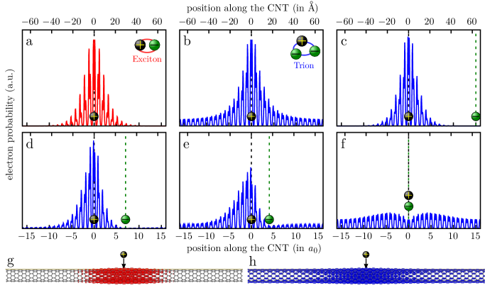
Figure 3: Spatial electron distribution in the exciton (red) and trion (blue) as a function of position along the CNT. (a) Spatial distribution of the electron relative to the hole, which is kept at the center of the panel (black vertical line), for the lowest-energy exciton. (b) Distribution of one electron relative to the hole (again in the center) for the lowest-energy trion, after complete spatial averaging over the other electron. (c)-(f) Distribution of one electron of the lowest-energy trion. The hole and the other electron are kept in the center (black vertical line) and at positions (indicated by the green vertical line) of 15, 7, 4, and 0 lattice constants $a_{0}$ (63 Å, 30 Å, 17 Å, and 0 Å) away from the hole. All distribution functions are given by $|\Phi|^{2}$ of the wave functions of Eq. (Three-particle correlation from a Many-Body Perspective: Trions in a Carbon Nanotube) and analog for excitons Note (1). All positions are on a line parallel to the CNT, at a distance of $3.7$ Å from its axis (i.e. on the outside of the CNT, $0.55$ Å above the nuclei, see also yellow line in (g) and (f)). (g)-(h) Three-dimensional view of the electron distribution, see (a) and (b).

Detailed information about spatial correlation can be obtained from the wave function (Three-particle correlation from a Many-Body Perspective: Trions in a Carbon Nanotube). Here we focus on the dark lowest-energy states. The wave function of the first bright exciton and trion look similar. Because of the six-/nine-dimensional nature of the exciton/trion wave functions, we discuss some characteristic features, only. Figs. 3 a and g show the probability distribution of the electron in the exciton state along the CNT, relative to the hole which is fixed in the center of the panel. Figs. 3 b and h exhibit the same quantity for the trion, after averaging over the coordinates of one of the two electrons. Figs. 3 b and h thus show the correlation of any of the two electrons to the hole. Due to the electron-hole attraction, the localization around the hole is still quite strong but farther extended (in real space) than for the exciton, resulting from the electron-electron repulsion. In particular, the envelope function does not decay to zero at large distance, but converges to the CBM wave function: at large distance, one electron observes attraction to the hole and repulsion from the other electron simultaneously, which cancel such that some free-electron mobility remains. The larger spatial extent of the electrons corresponds to stronger localization in reciprocal space as compared to the electron in the exciton state (see Fig. 2). In contrast, the reciprocal-space distribution of the hole is nearly the same for exciton and trion.

Further details of the trion become visible in Figs. 3 c-f where the hole and one electron are kept fixed (marked by a black line in the center and by a green line at various distances from the center of each panel), showing the spatial distribution of the other electron. In panel c the first electron is so far away from the hole that the same electron-hole pair distribution as for the exciton emerges. In panel d the second electron observes repulsion from the first electron (which is $30$ Å away from the hole) and tends to swerve to the left. This becomes even more pronounced when the fixed electron approaches the hole further (panel e). Here their distance of $17$ Å is already smaller than the intrinsic size of the exciton, so the above-mentioned free-particle behaviour of the other electron becomes visible. At even closer electron-hole distance (panel f), the other electron behaves as a free particle which is attractively scattered at the electron-hole pair. Note that in all cases the Pauli principle suppresses the amplitude of the two electrons at the same position (if they have the same spin), resulting e.g. in the dip in the center of panel f.

In summary, we have introduced a novel ab-initio scheme that accounts for many-body effects, which enables us to accurately describe trions and directly compare them to excitons. It further allows studying in detail the mechanisms of inter-particle correlation and entanglement on the atomic level. We have applied this method to negatively charged excitons (trions) in a semiconducting (8,0) CNT. A variety of trion states with different binding energies are found, e.g., $\sim$20 meV for the lowest dark and $\sim$130 meV for the lowest bright trion. The latter dominates luminescence which is red-shifted compared to the excitons, confirming experimental observations. Our data allows a detailed description of the internal energetics of trion states, their correlated composition from the single-particle states, and their spatial wave functions on a microscopic level. The latter demonstrate how quantum-mechanical correlation works on the atomic scale in nanostructured condensed matter. The presented method is generally applicable to all nanostructures and the obtained results are a further step towards a deeper understanding of three particle correlation and towards a specific manipulation of the latter by light and by charging, e.g., due to an externally applied gate voltage.

We thank P. Krüger for fruitful discussions and for critically reading our manuscript. The authors gratefully acknowledge the computing time granted by the John von Neumann Institute for Computing (NIC) and provided on the super-computer JURECA at Jülich Supercomputing Centre (JSC).

Supplement to
Three-particle correlation from a Many-Body Perspective:
Trions in a Carbon Nanotube

I Many-body approach towards three correlated particles

Ab-initio many-body perturbation theory (MBPT) is a state of the art method to reliably describe excited electronic states in electronic-structure theory Onida et al. (2002); Rohlfing and Louie (2000). Here we first briefly outline MBPT for electron-hole pairs for comparison and to provide a common notation. Thereafter corresponding issues for two electrons are outlined, followed by the discussion of trionic states for two electrons and one hole. The discussion is carried out in second quantization and kept very brief and simple, for explanatory purpose. Before deriving the Hamilton matrices in our many-body approach, Hartree-Fock theory is used for explanatory reasons only.

The formal description of correlated particles follows general concepts Combescot (2003); Combescot and Tribollet (2003); Esser et al. (2001) that have been employed for, e.g., semiconductor quantum dots Esser et al. (2000); Filinov et al. (2004); Narvaez et al. (2005); Rabani and Baer (2008); Huneke et al. (2011); Machnikowski and Kuhn (2011). Here we present the following derivations and formulas to have a consistent notation to extend it. Our many-body approach adds two essential features to those approaches: (i) We incorporate inhomogeneous and anisotropic dielectric screening $\epsilon({\bf r},{\bf r}^{\prime})$ on the atomic scale, rather than using a dielectric constant $\epsilon$ or a simple distance dependence $\epsilon(|{\bf r}-{\bf r}^{\prime}|)$. (ii) The band-structure energies and the screened Coulomb interaction between the particles both result from the same $GW$ self-energy operator (which incorporates dielectric screening) and must be evaluated on equal footing.

I.1 Electron-hole pair states

Within second-quantization notation, the ground state for an $N$-electron system may be denoted as $|0\rangle$. The application of annihilation and creation operators generates an electron-hole pair configuration as

$$|{\bf v}{\bf c}\rangle:=\hat{a}^{\dagger}_{\bf c}\hat{a}_{\bf v}|0\rangle~{}.$$ (S1)

In here, ${\bf v}$ (${\bf c}$) denotes occupied valence (empty conduction) states. For a periodic system ${\bf v}=(v,{\bf k}_{v}$) and ${\bf c}=(c,{\bf k}_{c}$) combine the band index ($v$, $c$) with a wave number (${\bf k}_{v}$, ${\bf k}_{c}$) for holes and electrons. Here we prefer the short-hand notation ${\bf v}$ (${\bf c}$) for the sake of brevity.

Within Hartree-Fock theory, the single-particle states $\phi_{\bf n}(x)$ are considered to be the solutions of the Hartree-Fock equations (i.e. $|0\rangle$ is taken as a single Slater determinant and minimizes the total energy of the system). The many-body Hamiltonian is then given as

$$\hat{H}=\sum_{{\bf ij}}h_{{\bf ij}}\hat{a}^{\dagger}_{\bf i}\hat{a}_{\bf j}+\frac{1}{2}\sum_{{\bf ijmn}}V_{{\bf ij},{\bf mn}}~{}\hat{a}^{\dagger}_{\bf i}\hat{a}^{\dagger}_{\bf j}\hat{a}_{\bf n}\hat{a}_{\bf m}$$ (S2)

with $h_{\bf ij}$ being the matrix elements of the single-particle terms (kinetic energy and external potential, e.g. pseudopotentials from the cores) and $V_{{\bf ij},{\bf mn}}$ being matrix elements of the Coulomb interaction:

$$V_{{\bf ij},{\bf mn}}=\int\phi_{\bf i}^{\ast}(x)\phi_{\bf j}^{\ast}(y)V(x,y)\phi_{\bf m}(x)\phi_{\bf n}(y)dxdy~{}.$$ (S3)

The coordinate $x=({\bf r},\sigma)$ combines position and spin; correspondingly, the integration includes spin summation, i.e. $\int dx=\sum_{\sigma=\pm}\int d^{3}r$. At the moment, the bare Coulomb interaction is considered, i.e. $V(x,x^{\prime})=e^{2}/|{\bf r}-{\bf r}^{\prime}|$. The implementation of screening effects (replacing $V$ by $W$) is discussed further below.

It turns out that the free electron-hole pair configurations $|{\bf v}{\bf c}\rangle$ are not eigenstates of the Hamiltonian (S2), because the matrix elements between two configurations $|{\bf v}{\bf c}\rangle$ and $|{\bf v}^{\prime}{\bf c}^{\prime}\rangle$ are non-diagonal:

$$\langle{\bf v}{\bf c}|\hat{H}|{\bf v}^{\prime}{\bf c}^{\prime}\rangle= (E_{0}^{({\rm HF})}+\epsilon^{({\rm HF})}_{\bf c}-\epsilon^{({\rm HF})}_{\bf v})\delta_{{\bf c}{\bf c}^{\prime}}\delta_{{\bf v}{\bf v}^{\prime}}$$

$$-(V_{{\bf v}^{\prime}{\bf c},{\bf v}{\bf c}^{\prime}}-V_{{\bf v}^{\prime}{\bf c},{\bf c}^{\prime}{\bf v}})$$ (S4)

with $\epsilon^{({\rm HF})}_{n}$ being the (Hartree-Fock) band-structure energy of level $n$. The Hartree-Fock ground-state energy $E_{0}^{({\rm HF})}$ can be disregarded in the following. Excited states result as linear combinations of the free electron-hole pair configurations, given by the diagonalization of the Hamilton matrix of Eq. (I.1):

$$|S,{\bf Q}\rangle=\sum_{{\bf v}{\bf c}}B^{(S,{\bf Q})}_{{\bf v}{\bf c}}|{\bf v}{\bf c}\rangle$$ (S5)

with the coefficients $B^{(S,{\bf Q})}_{{\bf v}{\bf c}}$ and the excitation energy $\Omega^{(S,{\bf Q})}$ of excitation $|S,{\bf Q}\rangle$ resulting from the eigenvalue equation

$$\sum_{{\bf v}^{\prime}{\bf c}^{\prime}}\langle{\bf v}{\bf c}|\hat{H}|{\bf v}^{\prime}{\bf c}^{\prime}\rangle B^{(S,{\bf Q})}_{{\bf v}^{\prime}{\bf c}^{\prime}}=\Omega^{(S,{\bf Q})}B^{(S,{\bf Q})}_{{\bf v}{\bf c}}~{}.$$ (S6)

These coupled states are the true electron-hole excitations (i.e., excitons in periodic systems). Note that the discussion here is restricted to the Tamm-Dancoff approximation within time-dependent Hartree-Fock theory. Eqs. (S5) and (S6) contain the total momentum Q of the exciton, which (according to Bloch’s theorem) is a good quantum number of the exciton and can be preselected. Accordingly, the summations in Eqs. (S5) and (S6), which contain double summations over ${\bf k}_{v}$ and ${\bf k}_{c}$, are restricted to such ${\bf k}_{v}$ that fulfill ${\bf k}_{v}={\bf k}_{c}-{\bf Q}$.

The electron-hole pair configurations yield a real-space amplitude of

$$\Phi_{{\bf v}{\bf c}}(x_{h},x_{e})=\langle 0|\hat{\psi}^{\dagger}(x_{h})\hat{\psi}(x_{e})|{\bf v}{\bf c}\rangle=\phi_{\bf v}^{\ast}(x_{h})\phi_{\bf c}(x_{e})$$ (S7)

(employing annihilation and creation field operators, with $x_{h}$ and $x_{e}$ denoting the coordinates of the hole and the electron), with a corresponding linear combination for a coupled state $|S,{\bf Q}\rangle$:

$$\Phi^{(S,{\bf Q})}(x_{h},x_{e})=\sum_{{\bf v}{\bf c}}B^{(S,{\bf Q})}_{{\bf v}{\bf c}}\phi_{\bf v}^{\ast}(x_{h})\phi_{\bf c}(x_{e})$$ (S8)

(again with the restriction ${\bf k}_{v}={\bf k}_{c}-{\bf Q}$ in the summation).

Furthermore, optical dipole transitions between the ground state and an excited state are controlled by the dipole-moment operator, $\hat{{\bf p}}=\sum_{\bf ij}{\bf p}_{\bf ij}\hat{a}^{\dagger}_{\bf i}\hat{a}_{\bf j}$, yielding

$$\langle 0|\hat{{\bf p}}|{\bf v}{\bf c}\rangle = {\bf p}_{{\bf v}{\bf c}}$$ (S9)

$$\langle 0|\hat{{\bf p}}|{S,{\bf Q}}\rangle = \sum_{{\bf v}{\bf c}}B^{(S,{\bf Q})}_{{\bf v}{\bf c}}{\bf p}_{{\bf v}{\bf c}}~{}.$$ (S10)

Note that only states with ${\bf Q}=0$ yield a non-zero dipole moment.

A formula similar to Eq. (I.1) can be derived independently within many-body perturbation theory. However, two important changes result from the consideration of dielectric screening effects: (i) the Hartree-Fock energy levels are replaced by quasiparticle levels $\epsilon_{\bf n}$ from a $GW$ calculation, and (ii) the interaction matrix elements between the electron-hole pair configurations becomes screened in the direct interaction part. We thus obtain an effective Hamiltonian for electron-hole pair states:

$$\langle{\bf v}{\bf c}|\hat{H}^{(eh)}|{\bf v}^{\prime}{\bf c}^{\prime}\rangle=(\epsilon_{{\bf c}}-\epsilon_{\bf v})\delta_{{\bf c}{\bf c}^{\prime}}\delta_{{\bf{\bf v}}{\bf{\bf v}}^{\prime}}-(W_{{\bf v}^{\prime}{\bf c},{\bf v}{\bf c}^{\prime}}-V_{{\bf v}^{\prime}{\bf c},{\bf c}^{\prime}{\bf v}})$$ (S11)

which is employed in the well established $GW$/BSE method. The matrix elements $W_{\bf ij,mn}$ have the same structure as Eq. (S3), but with the screened Coulomb interaction $W(x,x^{\prime})$ which includes dielectric screening effects in terms of the (inverse) dielectric function of the system via $W({\bf r},{\bf r}^{\prime})=\int\epsilon^{-1}({\bf r},{\bf r}^{\prime\prime})V({\bf r}^{\prime\prime},{\bf r}^{\prime})d^{3}r^{\prime\prime}$. As in most $GW$/BSE studies, we use dynamic screening in the $GW$, but restrict ourselves to static screening in the BSE. Note that within MBPT the exchange interaction between electrons and holes results from the classical part of the (bare) Coulomb interaction and is therefore not screened.

I.2 Correlated states of two electrons

As a preparation for trion states, we take an intermediate step and discuss states in which two electrons are moving in the conduction bands. An independent-particle configuration would be given by

$$|{\bf c}_{1}{\bf c}_{2}\rangle:=\hat{a}^{\dagger}_{{\bf c}_{2}}\hat{a}^{\dagger}_{{\bf c}_{1}}|0\rangle~{}.$$ (S12)

To avoid double counting, we require that ${\bf c}_{1}<{\bf c}_{2}$. This assumes that the empty states are ordered. The definition of the order is arbitrary (in particular when ${\bf c}=(c,{\bf k}_{c}$) includes a wave number) but has to be kept.

Within Hartree-Fock theory, the configurations (S12) are again not eigenstates of the Hamiltonian (S2). In fact, the Hamilton matrix elements between such configurations result as

$$\langle{\bf c}_{1}{\bf c}_{2}|\hat{H}|{\bf c}_{1}^{\prime}{\bf c}_{2}^{\prime}\rangle= (E_{0}^{({\rm HF})}+\epsilon^{({\rm HF})}_{{\bf c}_{1}}+\epsilon^{({\rm HF})}_{{\bf c}_{2}})\delta_{{\bf c}_{1}{\bf c}_{1}^{\prime}}\delta_{{\bf c}_{2}{\bf c}_{2}^{\prime}}$$

$$+(V_{{\bf c}_{1}{\bf c}_{2},{\bf c}_{1}^{\prime}{\bf c}_{2}^{\prime}}-V_{{\bf c}_{1}{\bf c}_{2},{\bf c}_{2}^{\prime}{\bf c}_{1}^{\prime}})~{}.$$ (S13)

The diagonalization of Eq. (I.2) yields correlated electron-electron pair states.

The two-electron states (S12) have a real-space amplitude of

$$\Phi_{{\bf c}_{1}{\bf c}_{2}}(x_{1},x_{2}) =\frac{1}{\sqrt{2}}\langle 0|\hat{\psi}(x_{1})\hat{\psi}(x_{2})|{\bf c}_{1}{\bf c}_{2}\rangle$$

$$=\frac{1}{\sqrt{2}}\{\phi_{{\bf c}_{1}}(x_{1})\phi_{{\bf c}_{2}}(x_{2})-\phi_{{\bf c}_{2}}(x_{1})\phi_{{\bf c}_{1}}(x_{2})\}$$ (S14)

(with $x_{1}$ and $x_{2}$ being the coordinates of the two electrons) which reflects the anti-symmetry required from two identical particles (including the vanishing of the wave function for $x_{1}=x_{2}$, i.e. same position and spin).

For physical correspondence to Eq. (S11) we again replace the Hartree-Fock levels by QP energy levels (also stemming from the $GW$ approach) and screen the interaction. We thus obtain an effective Hamiltonian for electron-electron pair states:

$$\langle{\bf c}_{1}{\bf c}_{2}|\hat{H}^{(ee)}|{\bf c}_{1}^{\prime}{\bf c}_{2}^{\prime}\rangle= (\epsilon_{{\bf c}_{1}}+\epsilon_{{\bf c}_{2}})\delta_{{\bf c}_{1}{\bf c}_{1}^{\prime}}\delta_{{\bf c}_{2}{\bf c}_{2}^{\prime}}$$

$$+(W_{{\bf c}_{1}{\bf c}_{2},{\bf c}_{1}^{\prime}{\bf c}_{2}^{\prime}}-W_{{\bf c}_{1}{\bf c}_{2},{\bf c}_{2}^{\prime}{\bf c}_{1}^{\prime}})~{}.$$ (S15)

Note that both interaction terms are screened. This is necessary to guarantee invariance of the entire approach when the order of the single-particle states (see at the beginning of this subsection) is selected in a different way.

I.3 Trion states of two electrons and one hole

As a direct extension of Secs. I.1 and I.2, independent-particle configurations of two electrons and one hole are constructed as

$$|{\bf v}{\bf c}_{1}{\bf c}_{2}\rangle:=\hat{a}^{\dagger}_{{\bf c}_{2}}\hat{a}^{\dagger}_{{\bf c}_{1}}\hat{a}_{\bf v}|0\rangle$$ (S16)

with the restriction again that ${\bf c}_{1}<{\bf c}_{2}$ within the chosen order of the single-particle levels, to avoid double counting among the identical electrons.

Within the framework of Hartree-Fock theory, the matrix elements between these configurations are

$$\langle{\bf v}{\bf c}_{1}{\bf c}_{2}|\hat{H} |{\bf v}^{\prime}{\bf c}^{\prime}_{1}{\bf c}^{\prime}_{2}\rangle=$$

$$(E_{0}^{({\rm HF})}+\epsilon^{({\rm HF})}_{{\bf c}_{1}}+\epsilon^{({\rm HF})}_{{\bf c}_{2}}-\epsilon^{({\rm HF})}_{\bf v})\delta_{{\bf c}_{1}{\bf c}_{1}^{\prime}}\delta_{{\bf c}_{2}{\bf c}_{2}^{\prime}}\delta_{{\bf v}{\bf v}^{\prime}}$$

$$+ (V_{{\bf c}_{1}{\bf c}_{2},{\bf c}^{\prime}_{1}{\bf c}^{\prime}_{2}}-V_{{\bf c}_{1}{\bf c}_{2},{\bf c}^{\prime}_{2}{\bf c}^{\prime}_{1}})\delta_{{\bf v}{\bf v}^{\prime}}$$

$$- (V_{{\bf v}^{\prime}{\bf c}_{1},{\bf v}{\bf c}^{\prime}_{1}}-V_{{\bf v}^{\prime}{\bf c}_{1},{\bf c}^{\prime}_{1}{\bf v}})\delta_{{\bf c}_{2}{\bf c}_{2}^{\prime}}$$

$$- (V_{{\bf v}^{\prime}{\bf c}_{2},{\bf v}{\bf c}^{\prime}_{2}}-V_{{\bf v}^{\prime}{\bf c}_{2},{\bf c}^{\prime}_{2}{\bf v}})\delta_{{\bf c}_{1}{\bf c}_{1}^{\prime}}~{}.$$ (S17)

The interpretation of these terms is straight-forward: The first line of Eq. (I.3) describes independent motion of each particle in the system’s band structure, while the other terms describe the interaction (direct and exchange) between the two electrons, and between the hole and each of the electrons.

In accordance with Eqs. (S11) and (I.2) we employ an effective Hamiltonian for trion states as:

$$\langle{\bf v}{\bf c}_{1}{\bf c}_{2}|\hat{H}^{(eeh)}|{\bf v}^{\prime}{\bf c}^{\prime}_{1}{\bf c}^{\prime}_{2}\rangle =(\epsilon_{{\bf c}_{1}}+\epsilon_{{\bf c}_{2}}-\epsilon_{\bf v})\delta_{{\bf c}_{1}{\bf c}_{1}^{\prime}}\delta_{{\bf c}_{2}{\bf c}_{2}^{\prime}}\delta_{{\bf v}{\bf v}^{\prime}}$$

$$+(W_{{\bf c}_{1}{\bf c}_{2},{\bf c}^{\prime}_{1}{\bf c}^{\prime}_{2}}-W_{{\bf c}_{1}{\bf c}_{2},{\bf c}^{\prime}_{2}{\bf c}^{\prime}_{1}})\delta_{{\bf v}{\bf v}^{\prime}}$$

$$-(W_{{\bf v}^{\prime}{\bf c}_{1},{\bf v}{\bf c}^{\prime}_{1}}-V_{{\bf v}^{\prime}{\bf c}_{1},{\bf c}^{\prime}_{1}{\bf v}})\delta_{{\bf c}_{2}{\bf c}_{2}^{\prime}}$$

$$-(W_{{\bf v}^{\prime}{\bf c}_{2},{\bf v}{\bf c}^{\prime}_{2}}-V_{{\bf v}^{\prime}{\bf c}_{2},{\bf c}^{\prime}_{2}{\bf v}})\delta_{{\bf c}_{1}{\bf c}_{1}^{\prime}}~{},$$ (S18)

again, keeping the general form as in Eq. (I.3), but using $GW$ band-structure energies and a screened Coulomb interaction where necessary.

The Hamiltonian (I.3) also causes the formation of correlated states $|T,{\bf K}\rangle$ ($\hat{=}$ trions) between the configurations (S16), i.e.

$$|T,{\bf K}\rangle=\sum_{{\bf v}{\bf c}_{1}{\bf c}_{2}}A^{(T,{\bf K})}_{{\bf v}{\bf c}_{1}{\bf c}_{2}}|{\bf v}{\bf c}_{1}{\bf c}_{2}\rangle~{}.$$ (S19)

Note that the summation is restricted to ${\bf c}_{1}<{\bf c}_{2}$ (see above). Here, ${\bf K}$ denotes the total momentum of the trion state (which, similar to excitons, is a good quantum number following Bloch’s theorem). Since the wave numbers of the contributing configurations $({\bf v}{\bf c}_{1}{\bf c}_{2})$ have to fulfill the requirement ${\bf k}_{v}={\bf k}_{1}+{\bf k}_{2}-{\bf K}$, the sum in Eq. (S19) is reduced.

Similar to excitons and electron-electron states, a configuration (S16) has a real-space amplitude

$$\Phi_{{\bf v}{\bf c}_{1}{\bf c}_{2}}(x_{h},x_{1},x_{2})=\frac{1}{\sqrt{2}}\langle 0|\hat{\psi}^{\dagger}(x_{h})\hat{\psi}(x_{1})\hat{\psi}(x_{2})|{\bf v}{\bf c}_{1}{\bf c}_{2}\rangle$$

$$\qquad=\phi_{\bf v}^{\ast}(x_{h})\frac{1}{\sqrt{2}}\left\{\phi_{{\bf c}_{1}}(x_{1})\phi_{{\bf c}_{2}}(x_{2})-\phi_{{\bf c}_{2}}(x_{1})\phi_{{\bf c}_{1}}(x_{2})\right\}$$ (S20)

(with $x_{h}$, $x_{1}$ and $x_{2}$ being the coordinates of the hole and the two electrons) and the corresponding linear combination for the trion state, is given by

$$\Phi^{(T,{\bf K})}(x_{h},x_{1},x_{2})=\sum_{{\bf v}{\bf c}_{1}{\bf c}_{2}}A^{(T,{\bf K})}_{{\bf v}{\bf c}_{1}{\bf c}_{2}}\phi_{\bf v}^{\ast}(x_{h})\times$$

$$\qquad\qquad\times\frac{1}{\sqrt{2}}\left\{\phi_{{\bf c}_{1}}(x_{1})\phi_{{\bf c}_{2}}(x_{2})-\phi_{{\bf c}_{2}}(x_{1})\phi_{{\bf c}_{1}}(x_{2})\right\}~{}.$$ (S21)

The expansion coefficients $A^{(T,{\bf K})}_{{\bf v}{\bf c}_{1}{\bf c}_{2}}$ and the energy $E^{(T,{\bf K})}$ of a trion $(T,{\bf K})$ result from the eigenvalue problem

$$\sum_{{\bf v}^{\prime}{\bf c}_{1}^{\prime}{\bf c}_{2}^{\prime}}\langle{\bf v}{\bf c}_{1}{\bf c}_{2}|\hat{H}^{(eeh)}|{\bf v}^{\prime}{\bf c}^{\prime}_{1}{\bf c}^{\prime}_{2}\rangle A^{(T,{\bf K})}_{{\bf v}^{\prime}{\bf c}^{\prime}_{1}{\bf c}_{2}^{\prime}}=E^{(T,{\bf K})}A^{(T,{\bf K})}_{{\bf v}{\bf c}_{1}{\bf c}_{2}}~{}.$$ (S22)

Note that the energy $E^{(T,{\bf K})}$ is not a transition energy to occur in an (optical) spectrum. Such transitions (including absorption or emission of a photon) would occur between the trion $|T,{\bf K}\rangle$ and an electron in the conduction band $|c{\bf K}\rangle$ (i.e. the single electron from which the absorption process starts, or the single electron which remains after one electron and the hole of the trion have recombined). Note that the trion and the remaining electron must have the same wave number ${\bf K}$ to allow photon-assisted transitions between them. Consequently, (optical) transition energies would be given by

$$\Omega(|T,{\bf K}\rangle\leftrightarrow|c{\bf K}\rangle)=E^{(T,{\bf K})}-\epsilon_{c{\bf K}}~{}.$$ (S23)

This is associated with a dipole moment

$$\langle c{\bf K}|\hat{{\bf p}}|T,{\bf K}\rangle =\sum_{{\bf v}{\bf c}_{1}{\bf c}_{2}}A^{(T,{\bf K})}_{{\bf v}{\bf c}_{1}{\bf c}_{2}}\langle c{\bf K}|\hat{{\bf p}}|{\bf v}{\bf c}_{1}{\bf c}_{2}\rangle$$

$$=\sum_{{\bf v}{\bf c}_{1}{\bf c}_{2}}A^{(T,{\bf K})}_{{\bf v}{\bf c}_{1}{\bf c}_{2}}\left({\bf p}_{{\bf v}{\bf c}_{1}}\delta_{c{\bf K},{\bf c}_{2}}-{\bf p}_{{\bf v}{\bf c}_{2}}\delta_{c{\bf K},{\bf c}_{1}}\right)~{}.$$ (S24)

II Hardware requirements for the calculations

Due to the third particle, the configuration space is much larger for trions than for excitons. A precise analysis of the required hardware is therefore necessary.

The number of occupied bands included in Eq. (S19) is denoted as $N_{v}$, the unoccupied bands as $N_{c}$ and the number of ${\bf k}$-points as $N_{\bf k}$. The size of the trion Hamiltonian is $\sim\frac{1}{2}N_{v}\cdot N_{c}^{2}\cdot N_{\bf k}^{2}$ (instead of $N_{v}\cdot N_{c}\cdot N_{\bf k}$ for excitons), including the factor $\sim$1/2 from the restriction that ${\bf c}_{1}$$<$${\bf c}_{2}$ (see Sec. I.3). Therefore the full Hamilton matrix can only be stored in memory for very small systems.

In Eq. (I.3) all four terms (kinetic energy, electron-electron interaction and electron-hole interaction) include Kronecker deltas. This allows to index these combinations properly and therefore to reduce the number of floating point operations for every matrix-vector multiplication drastically, in analogy to commonly known sparse matrix operations. In addition, this makes it possible to restrict the memory requirement tremendously and to share it efficiently between the processors. The minimal required memory for non-zero elements of the Hamiltonian scales with $N_{c}^{2}\cdot(N_{c}^{2}+N_{v}^{2})\cdot N_{\bf k}^{3}$.

In the particular case of the (8,0) CNT, we usually employ $32$ ${\bf k}$-points, 16 valence bands (out of a total of 128 valence bands, including spin) and 16 conduction bands. In these calculations, less than one percent of the Hamilton matrix elements is non-zero. This causes memory requirements of about $33$ GB. When $64$ ${\bf k}$-points are employed, the requirement rises to about $262$ GB.

In addition, up to ten vectors (of the dimension of the Hamiltonian) are required for the iterative procedure of applying the Hamiltonian to states and for the evaluation of the spectrum (using, e.g., the Haydock method). For the determination of trion states by an iterative diagonalization, on the other hand, more vectors and therefore more memory is required. For example, the determination of the lowest 5000 trion states (i.e., all states below 2.2 eV in Fig. 1 of the main text) requires about $900$ GB of memory, again employing $32$ ${\bf k}$-points.

III Numerical results

The trion calculations are carried out in the framework of many-body perturbation theory. Therefore several steps are necessary, which will be discussed one after the other.

III.1 DFT calculations

As a basis for the many-body calculations of the (8,0) CNT we first carry out a DFT calculation to provide an optimized geometry, DFT wave functions, and their band-structure energies. The $(8,0)$ CNT consists of $32$ carbon atoms in the unit cell, the configuration is sketched in Fig. S1.

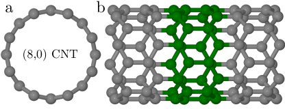
Figure S1: Structure of the (8,0) CNT. (a) Front view and (b) side view. The unit cell is marked in green.

The structure has eight-fold rotational symmetry along the tube axis, two mirror symmetries are observed perpendicular to it at the center and the border of the marked unit cell. the local density approximation (in the parametrization of Perdew and Zunger Perdew and Zunger (1981)). Norm-conserving pseudopotentials Hamann (1989) in Kleinman-Bylander form Kleinman and Bylander (1982) are used. We employ a mixed basis of 5 shells of Gaussian orbitals (38 functions with $s$, $p$, $d$, and $s^{\ast}$ symmetry, with decay constants from 0.1 to 3.0 $a_{B}^{-2}$) per carbon atom plus plane waves with a cutoff of $1$ Ry. The basis is unstable due to (almost) linear dependence among the basis functions. Stability is recovered by eliminating those linear combinations which are responsible for the instability, such that the resulting overlap matrix is again positive definite. A mesh of 16 ${\bf k}$-points in the one dimensional Brillouin zone is employed for the DFT. We obtain an optimized lattice constant of $4.22$ Å and a tube diameter of $6.29$ Å  after full relaxation of the structure. We employ a large unit cell perpendicular to the tube axis to guarantee a minimal distance of $10.6$ Å between the tubes. With this we obtain the eigenvalues and wave functions which serve as input for the $GW$ calculation.

III.2 $GW$ calculations

The MBPT calculations are carried out within the $GW$ approximation for the electron self energy. This requires a second, auxiliary basis set in which two-point quantities (e.g., the dielectric function, the screened Coulomb interaction etc.) are represented. Again, a mixed basis of 4 shells of Gaussian orbitals (34 functions with $s$, $p$, $d$, $s^{\ast}$, and $f$ symmetry, with decay constants from 0.25 to 4.0 $a_{B}^{-2}$) per carbon atom plus plane waves with a cutoff of $1$ Ry is used, which again has to be stabilized by elimination of linear dependence.

The main purpose of the $GW$ calculation is to provide the band-structure energies $\epsilon_{n,{\bf k}}$ required in Eqs. (S11) and (I.3), for the k-points in which the exciton and trion states are represented. The $GW$ self-energy operator further involves an integration in reciprocal space, which is carried out by a finite sum over q-points. For reasons of consistency with the BSE and trion calculation (see below) we employ a grid of q-points given by the differences between the k-points of the exciton (or trion) states. Obviously this difference grid includes the $\Gamma$ point (${\bf q}=0$), at which the Coulomb interaction diverges. We solve this problem by replacing the screened Coulomb interaction $W({\bf q}_{i})$ by its average $1/V_{i}\int_{V_{i}}W({\bf q})d^{3}q$ in the reciprocal volume $V_{i}$ of each grid point ${\bf q}_{i}$.

$GW$ calculations should include self-consistency in terms of the resulting band-structure energies. Here we simplify this requirement by including a scissors shift of $0.1$ Ry before the RPA screening and the $GW$ self-energy operator are evaluated. Thereby we anticipate the opening of the gap in a self-consistent approach. Comparing to this, our procedure is accurate to within 0.05 eV. Starting from a DFT-LDA gap of 0.58 eV, we finally obtain a $GW$ band gap of 1.70 eV. Similar results of $0.6$ eV (DFT) and $1.75$ eV ($GW$) have been found previously Spataru et al. (2004).

III.3 BSE calculations / optical absorption and luminescence spectra

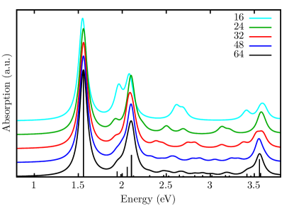
Figure S2: Exciton absorption spectrum. The spectra include different vertical offset to improve visibility. An artificial broadening of $0.054$ eV is employed.

The optical properties are then obtained by solving the BSE. We have tested convergence with respect to the k-points, using grids from 16 to 64 points. The resulting optical spectra are compiled in Fig. S2. We observe results converged better than $0.1$ eV even for meshes with only 16 ${\bf k}$-points. Especially the first optical peak at $1.56$ eV is very stable, as well as the first dark exciton at $1.090$ eV (not shown). Both this optical peak and the next one at $1.94$ eV are in good agreement with previous studies, as well as with experimental data (see Ref. Spataru et al. (2004); Chang et al. (2004); Rohlfing (2012); Mu et al. (2013)).

The calculation of luminescence spectra is analogous as explained in the next section (Eq. (S25)).

III.4 Trion calculations / optical absorption and luminescence spectra

In the last step we include an additional electron, and consider trion states as linear combinations of three-particle configurations. As described in Sec. II, the direct diagonalization of the trion Hamilton operator is not possible due to its high dimension ($\sim$10⁶), which depends on the number of bands and, in particular, on the number of k-points to be considered. For the evaluation of the optical spectrum the Haydock recursion method Haydock et al. (1972) and real-time integration followed by Fourier transform Schmidt et al. (2003) are a well established techniques. For the determination of a limited number of eigenstates at low energy, we employ iterative diagonalization techniques Hernandez et al. (2005, 2003). We have carefully checked the convergence behaviour of the spectra (using the Haydock method and using Fourier transform after real-time integration) and of the eigenstates with respect to the k-point sampling (see Fig. S3). We have further checked that in the low-energy part of the spectrum (accessible by iterative diagonalization) the eigenstates and the Haydock method yield the same spectral data.

To converge the full trion spectrum a larger number of ${\bf k}$-points has to be used than for the excitons. Fortunately, the low-energy results from 32 ${\bf k}$-point are already reasonably well converged (in comparison with data from larger sets, as shown in Fig. S3).

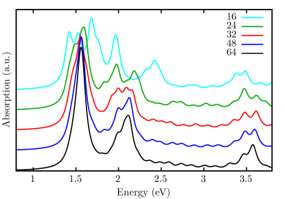
Figure S3: Trion absorption spectrum obtained using the Haydock recursion method. The spectra include different vertical offset to improve visibility. An artificial broadening of $0.054$ eV is used.

In analogy to the dipole moment for an exciton (see Eq. (S10)) the optical dipole moment for a trion are calculated by Eq. (S24). Note that in contrast to excitons, the initial (or final) state from (or to) which a transition occurs is not the ground state $|0\rangle$ but a single-electron state in a conduction band, $|c{\bf K}\rangle$. Due to momentum conservation in the optical transition, this electron’s momentum must equal the trion momentum, K. For Fig. S3 we have chosen ${\bf K}=0$, and the single-electron initial/final state is the CBM.

Although the spectra from various k-point grids are in reasonable agreement with each other, their exact shape slightly depends on the ${\bf k}$-point mesh, in particular at higher energy. Fortunately, the behaviour of the low-energy states is very stable. Fig. S4 shows the convergence of two excitons and of the related trions with respect to the grid density. In particular the energies of the lowest-energy trion (at 1.1 eV) and of the lowest dipole-allowed trion (at 1.4 eV) are very stable, similar to the excitons.

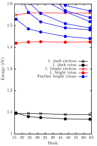
Figure S4: Convergence of the trion states with respect to the number of ${\bf k}$-points. The first dark (bright) exciton and trion are marked by black (red) crosses and dots. In addition, further trions (that are found in the manageable number of lowest states) are indicated by blue dots.

Optical absorption due to trions starts from a single-electron state and ends in a trion state. In contrast, luminescence (see Fig. 1 b of the main text) starts from the trions and ends in a single-electron state $|c{\bf K}\rangle$, again conserving total momentum. In this context several issues have to be considered. First, after the original excitation process the trions will (after some time) equilibrate according to the system’s temperature. By including a temperature-dependent Boltzmann distribution, we obtain a luminescence spectrum

$$L(E)\propto\sum_{c,{\bf K},|T,{\bf K}\rangle}\text{e}^{-\beta E^{(T,{\bf K})}} |\langle c{\bf K}|\hat{{\bf p}}|T,{\bf K}\rangle|^{2}\times$$

$$\times\delta(E- \Omega(|T,{\bf K}\rangle\leftrightarrow|c{\bf K}\rangle))$$ (S25)

with $\beta=1/(k_{B}T)$. Secondly, this expression requires to consider all possible momenta K and final-state band indices $c$. However, we find in our calculations that the dipole moments are particularly strong near ${\bf K}=0$ and quickly decrease for ${\bf K}\neq 0$. Furthermore, $E^{(T,{\bf K})}$ increases for ${\bf K}\neq 0$, leading to a decreasing Boltzmann factor and decreasing contribution to Eq. (S25). We have found that focusing on ${\bf K}=0$ is sufficient, since the inclusion of other momenta has no recognizable effect on the luminescence spectrum at room temperature. It should also be noted that the optically allowed trions near 1.4 eV show strong dipoles only for $c=\text{CBM}$ (i.e., the remaining electron in the lowest conduction band) and much smaller contribution from other bands. Transitions to higher bands $c$ occur at lower energy, but are dipole forbidden in the present case.

References

- Matsunaga et al. (2011) Ryusuke Matsunaga, Kazunari Matsuda, and Yoshihiko Kanemitsu, “Observation of Charged Excitons in Hole-Doped Carbon Nanotubes Using Photoluminescence and Absorption Spectroscopy,” Phys. Rev. Lett. 106, 037404 (2011).
- Santos et al. (2011) Silvia M. Santos, Bertrand Yuma, Stéphane Berciaud, Jonah Shaver, Mathieu Gallart, Pierre Gilliot, Laurent Cognet, and Brahim Lounis, “All-Optical Trion Generation in Single-Walled Carbon Nanotubes,” Phys. Rev. Lett. 107, 187401 (2011).
- Park et al. (2012) Jin Sung Park, Yasuhiko Hirana, Shinichiro Mouri, Yuhei Miyauchi, Naotoshi Nakashima, and Kazunari Matsuda, “Observation of Negative and Positive Trions in the Electrochemically Carrier-Doped Single-Walled Carbon Nanotubes,” Journal of the American Chemical Society 134, 14461–14466 (2012).
- Jakubka et al. (2014) Florian Jakubka, Stefan B. Grimm, Yuriy Zakharko, Florentina Gannott, and Jana Zaumseil, “Trion Electroluminescence from Semiconducting Carbon Nanotubes,” ACS Nano 8, 8477–8486 (2014).
- Rønnow et al. (2009) Troels F. Rønnow, Thomas G. Pedersen, and Horia D. Cornean, “Stability of singlet and triplet trions in carbon nanotubes,” Physics Letters A 373, 1478 – 1481 (2009).
- Rønnow et al. (2010) Troels F. Rønnow, Thomas G. Pedersen, and Horia D. Cornean, “Correlation and dimensional effects of trions in carbon nanotubes,” Phys. Rev. B 81, 205446 (2010).
- Watanabe and Asano (2012) Kouta Watanabe and Kenichi Asano, “Trions in semiconducting single-walled carbon nanotubes,” Phys. Rev. B 85, 035416 (2012).
- Nishihara et al. (2013) Taishi Nishihara, Yasuhiro Yamada, Makoto Okano, and Yoshihiko Kanemitsu, “Trion formation and recombination dynamics in hole-doped single-walled carbon nanotubes,” Applied Physics Letters 103 (2013), 10.1063/1.4813014.
- Yuma et al. (2013) B. Yuma, S. Berciaud, J. Besbas, J. Shaver, S. Santos, S. Ghosh, R. B. Weisman, L. Cognet, M. Gallart, M. Ziegler, B. Hönerlage, B. Lounis, and P. Gilliot, “Biexciton, single carrier, and trion generation dynamics in single-walled carbon nanotubes,” Phys. Rev. B 87, 205412 (2013).
- Mouri et al. (2013a) Shinichiro Mouri, Yuhei Miyauchi, Munechiyo Iwamura, and Kazunari Matsuda, “Temperature dependence of photoluminescence spectra in hole-doped single-walled carbon nanotubes: Implications of trion localization,” Phys. Rev. B 87, 045408 (2013a).
- Koyama et al. (2013) Takeshi Koyama, Satoru Shimizu, Yasumitsu Miyata, Hisanori Shinohara, and Arao Nakamura, “Ultrafast formation and decay dynamics of trions in -doped single-walled carbon nanotubes,” Phys. Rev. B 87, 165430 (2013).
- Mak et al. (2013) Kin Fai Mak, Keliang He, Changgu Lee, Gwan Hyoung Lee, James Hone, Tony F. Heinz, and Jie Shan, “Tightly bound trions in monolayer MoS2,” Nat Mater 12, 207–211 (2013).
- Ross et al. (2013) Jason S. Ross, Sanfeng Wu, Hongyi Yu, Nirmal J. Ghimire, Aaron M. Jones, Grant Aivazian, Jiaqiang Yan, David G. Mandrus, Di Xiao, Wang Yao, and Xiaodong Xu, “Electrical control of neutral and charged excitons in a monolayer semiconductor,” Nat Commun 4, 1474 (2013).
- Mouri et al. (2013b) Shinichiro Mouri, Yuhei Miyauchi, and Kazunari Matsuda, “Tunable photoluminescence of monolayer mos2 via chemical doping,” Nano Letters 13, 5944–5948 (2013b).
- Berkelbach et al. (2013) Timothy C. Berkelbach, Mark S. Hybertsen, and David R. Reichman, “Theory of neutral and charged excitons in monolayer transition metal dichalcogenides,” Phys. Rev. B 88, 045318 (2013).
- Rohlfing and Louie (2000) Michael Rohlfing and Steven G. Louie, “Electron-hole excitations and optical spectra from first principles,” Phys. Rev. B 62, 4927–4944 (2000).
- Onida et al. (2002) Giovanni Onida, Lucia Reining, and Angel Rubio, “Electronic excitations: density-functional versus many-body Green’s-function approaches,” Rev. Mod. Phys. 74, 601–659 (2002).
- Note (1) See Supplementary Material for a detailed discussion of our theoretical framework and further numerical details at http://link.aps.org/supplemental/10.1103/PhysRevLett.116.196804, which includes Ref. Combescot (2003); Combescot and Tribollet (2003); Esser et al. (2001); Perdew and Zunger (1981); Hamann (1989); Kleinman and Bylander (1982); Hernandez et al. (2003).
- Strinati (1982) G. Strinati, “Dynamical Shift and Broadening of Core Excitons in Semiconductors,” Phys. Rev. Lett. 49, 1519–1522 (1982).
- Strinati (1984) G. Strinati, “Effects of dynamical screening on resonances at inner-shell thresholds in semiconductors,” Phys. Rev. B 29, 5718–5726 (1984).
- Esser et al. (2000) Axel Esser, Erich Runge, Roland Zimmermann, and Wolfgang Langbein, “Photoluminescence and radiative lifetime of trions in gaas quantum wells,” Phys. Rev. B 62, 8232–8239 (2000).
- Filinov et al. (2004) A. V. Filinov, C. Riva, F. M. Peeters, Yu. E. Lozovik, and M. Bonitz, “Influence of well-width fluctuations on the binding energy of excitons, charged excitons, and biexcitons in -based quantum wells,” Phys. Rev. B 70, 035323 (2004).
- Narvaez et al. (2005) Gustavo A. Narvaez, Gabriel Bester, and Alex Zunger, “Excitons, biexcitons, and trions in self-assembled quantum dots: Recombination energies, polarization, and radiative lifetimes versus dot height,” Phys. Rev. B 72, 245318 (2005).
- Rabani and Baer (2008) E. Rabani and R. Baer, “Distribution of Multiexciton Generation Rates in CdSe and InAs Nanocrystals,” Nano Letters 8, 4488–4492 (2008).
- Huneke et al. (2011) J. Huneke, I. D’Amico, P. Machnikowski, T. Thomay, R. Bratschitsch, A. Leitenstorfer, and T. Kuhn, “Role of coulomb correlations for femtosecond pump-probe signals obtained from a single quantum dot,” Phys. Rev. B 84, 115320 (2011).
- Machnikowski and Kuhn (2011) Paweł Machnikowski and Tilmann Kuhn, “Nonlinear optical response of hole–trion systems in quantum dots in tilted magnetic fields,” physica status solidi (c) 8, 1231–1234 (2011).
- Spataru et al. (2004) Catalin D. Spataru, Sohrab Ismail-Beigi, Lorin X. Benedict, and Steven G. Louie, “Excitonic Effects and Optical Spectra of Single-Walled Carbon Nanotubes,” Phys. Rev. Lett. 92, 077402 (2004).
- Chang et al. (2004) Eric Chang, Giovanni Bussi, Alice Ruini, and Elisa Molinari, “Excitons in carbon nanotubes: An Ab Initio symmetry-based approach,” Phys. Rev. Lett. 92, 196401 (2004).
- Mu et al. (2013) Jinglin Mu, Yuchen Ma, Huabing Yin, Chengbu Liu, and Michael Rohlfing, “Photoluminescence of Single-Walled Carbon Nanotubes: The Role of Stokes Shift and Impurity Levels,” Phys. Rev. Lett. 111, 137401 (2013).
- Rohlfing (2012) Michael Rohlfing, “Redshift of Excitons in Carbon Nanotubes Caused by the Environment Polarizability,” Phys. Rev. Lett. 108, 087402 (2012).
- Johnson and Hulbert (1987) P. D. Johnson and S. L. Hulbert, “Inverse-photoemission studies of adsorbed diatomic molecules,” Physical Review B 35, 9427–9436 (1987).
- Puschnig et al. (2012) Peter Puschnig, Peiman Amiri, and Claudia Draxl, “Band renormalization of a polymer physisorbed on graphene investigated by many-body perturbation theory,” Physical Review B 86, 085107 (2012).
- Milko et al. (2012) Matus Milko, Peter Puschnig, and Claudia Draxl, “Predicting the electronic structure of weakly interacting hybrid systems: The example of nanosized peapod structures,” Physical Review B 86, 155416 (2012).
- Milko et al. (2013) Matus Milko, Peter Puschnig, Pascal Blondeau, Enzo Menna, Jia Gao, Maria Antonietta Loi, and Claudia Draxl, “Evidence of Hybrid Excitons in Weakly Interacting Nanopeapods,” The Journal of Physical Chemistry Letters 4, 2664–2667 (2013).
- Neaton et al. (2006) J. B. Neaton, Mark S. Hybertsen, and Steven G. Louie, “Renormalization of Molecular Electronic Levels at Metal-Molecule Interfaces,” Phys. Rev. Lett. 97, 216405 (2006).
- Garcia-Lastra et al. (2009) J. M. Garcia-Lastra, C. Rostgaard, A. Rubio, and K. S. Thygesen, “Polarization-induced renormalization of molecular levels at metallic and semiconducting surfaces,” Physical Review B 80, 245427 (2009).
- Garcia-Lastra and Thygesen (2011) J.M. Garcia-Lastra and K.S. Thygesen, “Renormalization of Optical Excitations in Molecules near a Metal Surface,” Phys. Rev. Lett. 106, 187402 (2011).
- Haydock et al. (1972) R Haydock, V Heine, and M J Kelly, “Electronic structure based on the local atomic environment for tight-binding bands,” Journal of Physics C: Solid State Physics 5, 2845 (1972).
- Schmidt et al. (2003) W. G. Schmidt, S. Glutsch, P. H. Hahn, and F. Bechstedt, “Efficient method to solve the bethe-salpeter equation,” Phys. Rev. B 67, 085307 (2003).
- Hernandez et al. (2005) Vicente Hernandez, Jose E. Roman, and Vicente Vidal, “SLEPc: A scalable and flexible toolkit for the solution of eigenvalue problems,” ACM Trans. Math. Software 31, 351–362 (2005).
- Note (2) Sufficient processors and memory were supplied by the HPC system PALMA of the University of Münster and the super-computer JURECA at Jülich Supercomputing Centre (JSC).
- Note (3) Note that due to the involved approximations, the absolute accuracy of any /BSE study cannot be better than 0.1\tmspace+.1667emeV. On the other hand, relative energy differences between excitations and between excitons and trions can be given with much higher precision.
- Note (4) Note that the dynamical processes leading to thermal equilibrium, as well as details of the emission processes, are not considered here, so the amplitudes in the luminescence spectrum can only indicate trends.
- Combescot (2003) Monique Combescot, “Trions in first and second quantizations,” The European Physical Journal B - Condensed Matter and Complex Systems 33, 311–320 (2003).
- Combescot and Tribollet (2003) Monique Combescot and Jérôme Tribollet, “Trion oscillator strength,” Solid State Communications 128, 273 – 277 (2003).
- Esser et al. (2001) A. Esser, R. Zimmermann, and E. Runge, “Theory of trion spectra in semiconductor nanostructures,” physica status solidi (b) 227, 317–330 (2001).
- Perdew and Zunger (1981) J. P. Perdew and Alex Zunger, “Self-interaction correction to density-functional approximations for many-electron systems,” Phys. Rev. B 23, 5048–5079 (1981).
- Hamann (1989) D. R. Hamann, “Generalized norm-conserving pseudopotentials,” Phys. Rev. B 40, 2980–2987 (1989).
- Kleinman and Bylander (1982) Leonard Kleinman and D. M. Bylander, “Efficacious Form for Model Pseudopotentials,” Phys. Rev. Lett. 48, 1425–1428 (1982).
- Hernandez et al. (2003) V. Hernandez, J. E. Roman, and V. Vidal, “SLEPc: Scalable Library for Eigenvalue Problem Computations,” Lecture Notes in Computer Science 2565, 377–391 (2003).

References

- Onida et al. (2002) Giovanni Onida, Lucia Reining, and Angel Rubio, “Electronic excitations: density-functional versus many-body Green’s-function approaches,” Rev. Mod. Phys. 74, 601–659 (2002).
- Rohlfing and Louie (2000) Michael Rohlfing and Steven G. Louie, “Electron-hole excitations and optical spectra from first principles,” Phys. Rev. B 62, 4927–4944 (2000).
- Combescot (2003) Monique Combescot, “Trions in first and second quantizations,” The European Physical Journal B - Condensed Matter and Complex Systems 33, 311–320 (2003).
- Combescot and Tribollet (2003) Monique Combescot and Jérôme Tribollet, “Trion oscillator strength,” Solid State Communications 128, 273 – 277 (2003).
- Esser et al. (2001) A. Esser, R. Zimmermann, and E. Runge, “Theory of Trion Spectra in Semiconductor Nanostructures,” physica status solidi (b) 227, 317–330 (2001).
- Esser et al. (2000) Axel Esser, Erich Runge, Roland Zimmermann, and Wolfgang Langbein, “Photoluminescence and radiative lifetime of trions in gaas quantum wells,” Phys. Rev. B 62, 8232–8239 (2000).
- Filinov et al. (2004) A. V. Filinov, C. Riva, F. M. Peeters, Yu. E. Lozovik, and M. Bonitz, “Influence of well-width fluctuations on the binding energy of excitons, charged excitons, and biexcitons in -based quantum wells,” Phys. Rev. B 70, 035323 (2004).
- Narvaez et al. (2005) Gustavo A. Narvaez, Gabriel Bester, and Alex Zunger, “Excitons, biexcitons, and trions in self-assembled quantum dots: Recombination energies, polarization, and radiative lifetimes versus dot height,” Phys. Rev. B 72, 245318 (2005).
- Rabani and Baer (2008) E. Rabani and R. Baer, “Distribution of Multiexciton Generation Rates in CdSe and InAs Nanocrystals,” Nano Letters 8, 4488–4492 (2008).
- Huneke et al. (2011) J. Huneke, I. D’Amico, P. Machnikowski, T. Thomay, R. Bratschitsch, A. Leitenstorfer, and T. Kuhn, “Role of coulomb correlations for femtosecond pump-probe signals obtained from a single quantum dot,” Phys. Rev. B 84, 115320 (2011).
- Machnikowski and Kuhn (2011) Paweł Machnikowski and Tilmann Kuhn, “Nonlinear optical response of hole–trion systems in quantum dots in tilted magnetic fields,” physica status solidi (c) 8, 1231–1234 (2011).
- Perdew and Zunger (1981) J. P. Perdew and Alex Zunger, “Self-interaction correction to density-functional approximations for many-electron systems,” Phys. Rev. B 23, 5048–5079 (1981).
- Hamann (1989) D. R. Hamann, “Generalized norm-conserving pseudopotentials,” Phys. Rev. B 40, 2980–2987 (1989).
- Kleinman and Bylander (1982) Leonard Kleinman and D. M. Bylander, “Efficacious Form for Model Pseudopotentials,” Phys. Rev. Lett. 48, 1425–1428 (1982).
- Spataru et al. (2004) Catalin D. Spataru, Sohrab Ismail-Beigi, Lorin X. Benedict, and Steven G. Louie, “Excitonic Effects and Optical Spectra of Single-Walled Carbon Nanotubes,” Phys. Rev. Lett. 92, 077402 (2004).
- Chang et al. (2004) Eric Chang, Giovanni Bussi, Alice Ruini, and Elisa Molinari, “Excitons in Carbon Nanotubes: An Ab Initio Symmetry-Based Approach,” Phys. Rev. Lett. 92, 196401 (2004).
- Rohlfing (2012) Michael Rohlfing, “Redshift of Excitons in Carbon Nanotubes Caused by the Environment Polarizability,” Phys. Rev. Lett. 108, 087402 (2012).
- Mu et al. (2013) Jinglin Mu, Yuchen Ma, Huabing Yin, Chengbu Liu, and Michael Rohlfing, “Photoluminescence of Single-Walled Carbon Nanotubes: The Role of Stokes Shift and Impurity Levels,” Phys. Rev. Lett. 111, 137401 (2013).
- Haydock et al. (1972) R Haydock, V Heine, and M J Kelly, “Electronic structure based on the local atomic environment for tight-binding bands,” Journal of Physics C: Solid State Physics 5, 2845 (1972).
- Schmidt et al. (2003) W. G. Schmidt, S. Glutsch, P. H. Hahn, and F. Bechstedt, “Efficient method to solve the Bethe-Salpeter equation,” Phys. Rev. B 67, 085307 (2003).
- Hernandez et al. (2005) Vicente Hernandez, Jose E. Roman, and Vicente Vidal, “SLEPc: A Scalable and Flexible Toolkit for the Solution of Eigenvalue Problems,” ACM Trans. Math. Software 31, 351–362 (2005).
- Hernandez et al. (2003) V. Hernandez, J. E. Roman, and V. Vidal, “SLEPc: Scalable Library for Eigenvalue Problem Computations,” Lecture Notes in Computer Science 2565, 377–391 (2003).