Outlier Edge Detection Using Random Graph Generation Models and Applications

Abstract

Outliers are samples that are generated by different mechanisms from other normal data samples. Graphs, in particular social network graphs, may contain nodes and edges that are made by scammers, malicious programs or mistakenly by normal users. Detecting outlier nodes and edges is important for data mining and graph analytics. However, previous research in the field has merely focused on detecting outlier nodes. In this article, we study the properties of edges and propose outlier edge detection algorithms using two random graph generation models. We found that the edge-ego-network, which can be defined as the induced graph that contains two end nodes of an edge, their neighboring nodes and the edges that link these nodes, contains critical information to detect outlier edges. We evaluated the proposed algorithms by injecting outlier edges into some real-world graph data. Experiment results show that the proposed algorithms can effectively detect outlier edges. In particular, the algorithm based on the Preferential Attachment Random Graph Generation model consistently gives good performance regardless of the test graph data. Further more, the proposed algorithms are not limited in the area of outlier edge detection. We demonstrate three different applications that benefit from the proposed algorithms: 1) a preprocessing tool that improves the performance of graph clustering algorithms; 2) an outlier node detection algorithm; and 3) a novel noisy data clustering algorithm. These applications show the great potential of the proposed outlier edge detection techniques.

1 Introduction

Graphs are an important data representation, which have been extensively used in many scientific fields such as data mining, bioinformatics, multimedia content retrieval and computer vision. For several hundred years, scientists have been enthusiastic about graph theory and its applications [1]. Since the revolution of the computer technologies and the Internet, graph data have become more and more important because many of the “big” data are naturally formed in a graph structure or can be transformed into graphs.

Outliers almost always happen in real-world graphs. Outliers in a graph can be outlier nodes or outlier edges. For example, outlier nodes in a social network graph may include: scammers who steal users’ personal information; fake accounts that manipulate the reputation management system; or spammers who send free and mostly false advertisements [2, 3]. Researchers have been working on algorithms to detect these malicious outlier nodes in graphs [4, 5, 6, 7]. Outlier edges are also common in graphs. They can be edges that are generated by outlier nodes, or unintentional links made by normal users or the system. Outlier edges are not only harmful but also greatly increase the system complexity and degrade the performance of graph mining algorithms. In this paper, we will show that the performance of the community detection algorithms can be greatly improved when a small amount of outlier edges are removed. Outlier edge detection can also help evaluate and monitor the behavior of end users and further identify the malicious entities. However, in contrast to the focus on the outlier node detection, there have been very few studies on outlier edge detection.

In this paper, we present novel outlier edge detection algorithms. Our proposed algorithms use the clustering property of social network graphs to detect outlier edges. The outlier score of an edge is determined by the difference of the actual number of edges and the expected number of edges that link the two groups of nodes that are around the edge. We use random graph generation models to predict the number of edges between the two groups of nodes. We evaluated the proposed algorithms using injected edges in real-world graph data.

Further more, we show the great potentials of the outlier edge detection technique in the areas of graph mining and pattern recognition. We demonstrate three different applications that are based on the proposed algorithms: 1) a preprocessing tool for graph clustering algorithms; 2) an outlier node detection algorithm; 3) a novel noisy data clustering algorithm.

The rest of the paper is organized as follows: the prior art is reviewed in Section 2; the methodology to detect outlier edges is in Section 3; evaluation of the proposed algorithms are given in Section 4; various applications that use or benefit from outlier edge detection algorithms are presented in Section 5; and finally, conclusions and future directions are included in Section 6.

2 Previous Work

Outliers are data instances that are markedly different from the rest of the data [8]. Outliers are often located outside (mostly far way) from the normal data points when presented in an appropriate feature space. It is also commonly assumed that the number of outliers is much less than the number of normal data points.

Outlier detection in graph data includes outlier node detection and outlier edge detection. Noble and Cook studied substructures of graphs and used the Minimum Description Length technique to detect unusual patterns in a graph [5]. Xu et al. considered nodes that marginally connect to a structure (or community) as outliers [9]. They used a searching strategy to group the nodes that share many common neighbors into communities. The nodes that are not tightly connected to any community are classified as outliers. Gao et al. also studied the roles of the nodes in communities [10]. Nodes in a community tend to have similar attributes. Using the Hidden Markov Random Field technique as a generative model, they were able to detect the nodes that are abnormal in their community. Akoglu et al. detected outlier nodes using the near-cliques and stars, heavy vicinities and dominant heavy links properties of the ego-network–the induced network formed by a focal node and its direct neighbors [11]. They observed that some pairs of the features of normal nodes follow a power law and defined an outlier score function that measures the deviation of a node from the normal patterns. Dai et al. detected outlier nodes in bipartite graphs using mutual agreements between nodes [6].

In contrast to proliferative research on outlier node detection, there have been very few studies on outlier edge detection in graphs. Chakrabarti detected outlier edges by partitioning nodes into groups using the Minimum Description Length technique [12]. Edges that link the nodes from different groups are considered as outliers. These edges are also called weak links or weak ties in literature [13]. Obviously this method has severe limitations. First, one shall not classify all weak links as outliers since they are part of the normal graph data. Second, many outlier edges do not happen between the groups. Finally, many graphs do not contain easily partitionable groups.

Detection of missing edges (or link prediction) is the opposite technique of outlier edge detection. These algorithms find missing edges between pairs of nodes in a graph. They are critical in recommendation systems, especially in e-commerce industry and social network service industry [14, 15]. Such algorithms evaluate similarities between each pair of nodes. A pair of nodes with high similarity score is likely to be connected by an edge. One may use the similarity scores to detect outlier edges. The edges whose two end nodes have a low similarity score are likely to be the outlier edges. However, in practice, these similarity scores do not give satisfactory performance if one uses them to detect outlier edges.

3 Methodology

3.1 Notation

Let $G(V,E)$ denote a graph with a set of nodes $V$ and a set of edges $E$. In this article, we consider undirected, unweighted graphs that do not contain self-loops. We use lower case $a,\ b,\ c,$ etc., to represent nodes. Let $\overline{ab}$ denote the edge that connects nodes $a$ and $b$. Because our graph $G$ is undirected, $\overline{ab}$ and $\overline{ba}$ represent the same edge. Let $N_{a}$ be the set of neighboring nodes of node $a$, such that $N_{a}=\left\{x|x\in V,\overline{xa}\in E\right\}$. Let $S_{a}=N_{a}\cup\left\{a\right\}$ (i.e. $S_{a}$ contains node $a$ and its neighboring nodes). Let $k_{a}$ be the degree of node $a$, so that $k_{a}=\left|N_{a}\right|$. Let $A$ be the adjacency matrix of graph $G$. Let $n=\left|V\right|$ be the number of nodes and $m=\left|E\right|$ be the number of edges of graph $G$.

Freeman defines the ego-network as the induced subgraph that contains a focal node and all of its neighboring nodes together with edges that link these nodes [16]. To study the properties of an edge, we define the edge-ego-network as follows:

Definition 1.

An edge-ego-network is the induced subgraph that contains the two end nodes of an edge, all neighboring nodes of these two end nodes and all edges that link these nodes.

Let $G_{\overline{ab}}=G\left(V_{\overline{ab}},E_{\overline{ab}}\right)$ denote the edge-ego-network of edge $\overline{ab}$, where $V_{\overline{ab}}=S_{a}\cup S_{b}$ and $E_{\overline{ab}}=\left\{\overline{xy}|x\in V_{\overline{ab}},y\in V_{\overline{ab}}\ \mathrm{and}\ \overline{xy}\in E\right\}$.

3.2 Motivation

Graphs representing real-world data, in particular social network graphs, often exhibit the clustering property–nodes tend to form highly dense groups in a graph [17]. For example, if two people have many friends in common, they are likely to be friends too. Therefore, it is common for social network services to recommend new connections to a user using this clustering property [14]. As a consequence, social network graphs display an even stronger clustering property compared to other graphs. New connections to a node may be recommended from the set of neighboring nodes with the highest number of common neighbors to the given node. The common neighbors (CN) score of node $a$ and node $b$ is defined as

$$s_{CN}=\left|N_{a}\cap N_{b}\right|.$$ (1)

CN score is the basis of many node similarity scores that have been used to find missing edges [14]. Some common similarity indices are:

• Salton index or cosine similarity (Salton)

  $$s_{Salton}=\frac{S_{CN}}{\sqrt{k_{a}k_{b}}}$$ (2)

• Jaccard index (Jaccard)

  $$s_{Jaccard}=\frac{S_{CN}}{\left|N_{a}\cup N_{b}\right|}$$ (3)

• Hub promoted index (HPI)

  $$s_{HPI}=\frac{S_{CN}}{\min(k_{a},k_{b})}$$ (4)

• Hub depressed index (HDI)

  $$s_{HDI}=\frac{S_{CN}}{\max(k_{a},k_{b})}$$ (5)

Next we shall investigate how to detect outlier edges in a social network using the clustering property. According to this property, if two people are friends, they are likely to have many common friends or their friends are also friends of each other. If two people are linked by an edge, but do not share any common friends and neither do their friends know each other, we have good reason to suspect that the link between them is an outlier. So, when node $a$ and node $b$ are connected by edge $\overline{ab}$, there should be edges connect the nodes in set $S_{a}$ and the nodes in set $S_{b}$. However, the number of connections should depend on the number of nodes in these two groups. Let us consider the different cases as shown in Fig. 1.

(a)	(b)
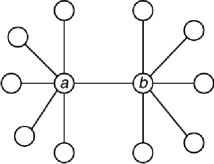
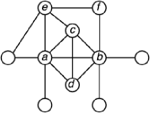
(c)	(d)

Figure 1: Different cases of edge-ego-networks (a) $k_{a}=k_{b}=1$, $\left|N_{a}\cap N_{b}\right|=0$ (b) $k_{a}=k_{b}=2$, $\left|N_{a}\cap N_{b}\right|=0$ (c) $k_{a}=k_{b}=6$, $\left|N_{a}\cap N_{b}\right|=0$ (d) $k_{a}=k_{b}=6$, $\left|N_{a}\cap N_{b}\right|=2$

In these four cases, edge $\overline{ab}$ is likely to be a normal edge in case (d) because nodes $a$ and $b$ share common neighboring nodes $c$ and $d$, and there are connections between neighboring nodes of $a$ and those of $b$. In the case of (a), (b) and (c), $\left|N_{a}\cap N_{b}\right|=0$, which implies that nodes $a$ and $b$ do not share any common neighboring nodes. However edge $\overline{ab}$ in case (c) is more likely to be an outlier edge because nodes $a$ and $b$ have each many neighboring nodes but there is no connection between any two of these neighboring nodes. In case (a) and (b) we do not have enough information to judge whether edge $\overline{ab}$ is an outlier edge or not. If we apply the node similarity scores to detect outlier edges, we find that $S_{CN}=0$ for cases (a), (b) and (c). Thus, the node similarity scores defined by Eqs. (1), (2), (3), (4) and (5) all equal to 0. For this reason, these node similarity scores cannot effectively detect outlier edges.

In case (c), edge $\overline{ab}$ is likely to be an outlier edge because the expected number of edges between node $a$ together with its neighboring nodes and node $b$ together with its neighboring nodes is high, whereas the actual number of edges is low. So, according to the clustering property, we propose the following definition for the edge outlier score:

Definition 2.

The outlier score of an edge is defined as the difference between the number of actual edges and the expected value of the number of edges that link the two sets of neighboring nodes of the two end nodes of the given edge. That is:

$$s_{\overline{ab}}=m_{\overline{ab}}-e_{\overline{ab}},$$ (6)

where $m_{\overline{ab}}$ is the actual number of edges that links the two sets of nodes–one set is node $a$ together with its neighboring nodes and the other set is node $b$ together with its neighboring nodes, and $e_{\overline{ab}}$ is the expected number of edges that link the aforementioned two sets of nodes.

We can rank the edges by their edge outlier scores defined in Eq. (6). The edges with low scores are more likely to be outlier edges in a graph.

Let $\alpha\left(S,T\right)=\left|\overline{ab}|a\in S,b\in T\ \mathrm{and}\ \overline{ab}\in E\right|$ denote the number of edges that links the nodes in sets $S$ and $T$. We suppose the graph $G$ is generated by a random graph generation model. Let $\epsilon\left(S,T\right)$ denote the expected value of the number of edges that links the nodes in sets $S$ and $T$ by the generation model. Section 3.4 describes two generation models and the functions of calculating $\epsilon\left(S,T\right)$. Obviously $\alpha\left(S,T\right)$ and $\epsilon\left(S,T\right)$ are symmetric functions. That is:

Theorem 3.

$\alpha\left(S,T\right)=\alpha\left(T,S\right)$ and $\epsilon\left(S,T\right)=\epsilon\left(T,S\right)$.

Let $P_{a,b}$ and $R_{a,b}$ be the two sets of nodes that are related to end nodes $a$ and $b$. Node set $R_{a,b}$ depends on set $P_{a,b}$. The actual number of edges and the expected number of edges of the sets of nodes related to the two end nodes may vary when we switch the end nodes $a$ and $b$. We use the following equations to calculate $m_{\overline{ab}}$ and $e_{\overline{ab}}$:

$$m_{\overline{ab}}=\frac{1}{2}\left(\alpha\left(P_{a,b},R_{a,b}\right)+\alpha\left(P_{b,a},R_{b,a}\right)\right);$$ (7)

$$e_{\overline{ab}}=\frac{1}{2}\left(\epsilon\left(P_{a,b},R_{a,b}\right)+\epsilon\left(P_{b,a},R_{b,a}\right)\right).$$ (8)

3.3 Schemes of Node Neighborhood Sets

For a ego-network, Coscia and Rossetti showed the importance of removing the focal node and all edges that link to it when studying the properties of ego-networks [18]. It is more complicate to study the properties of an edge-ego-network since there are two ending nodes and two sets of neighboring nodes involved. Considering the common nodes of the neighboring nodes and the end nodes of the edge being investigated, we now define four schemes that capture different configurations of these two sets.

Let $S_{a\backslash b}=S_{a}\backslash\left\{b\right\}$ be the set of nodes that contains node $a$ and its neighboring nodes except node $b$. Let $N_{a\backslash b}=N_{a}\backslash\left\{b\right\}$ be the set of nodes that contains the neighboring nodes of $a$ except node $b$. Obviously $S_{a\backslash b}=N_{a\backslash b}\cup\left\{a\right\}$. Fig. 2 shows the edge-ego-network $G_{\overline{ab}}$ and the two sets of nodes $S_{a\backslash b}$ and $S_{b\backslash a}$ corresponding to case (d) in Fig. 1.

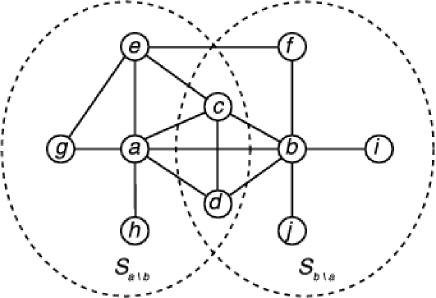
Figure 2: The sets of the nodes of the edge-ego-network $G_{\overline{ab}}$ in the case (d) of Fig. 1

We first define two sets of nodes that are related to node $a$ and its neighboring nodes: $N_{a\backslash b}$ and $S_{a\backslash b}$. Next, we define two sets of nodes that are related to node $b$ and its neighboring nodes with regard to the sets of nodes $N_{a\backslash b}$ and $S_{a\backslash b}$: $S_{b\backslash a}\backslash S_{a\backslash b}$ and $S_{b\backslash a}$. In Fig. 2, $N_{a\backslash b}=\left\{c,d,e,g,h\right\}$, $S_{a\backslash b}=\left\{a,c,d,e,g,h\right\}$, $S_{b\backslash a}\backslash S_{a\backslash b}=\left\{b,f,i,j\right\}$ and $S_{b\backslash a}=\left\{b,c,d,f,i,j\right\}$. In the case of a social network graph, $N_{a\backslash b}$ would consist of friends of user (node) $a$ except $b$; $S_{a\backslash b}$ consists of $a$ and friends of $a$ except $b$; $S_{b\backslash a}\backslash S_{a\backslash b}$ consists of $b$ and friends of $b$ except $a$ and those who are friends of $a$; $S_{b\backslash a}$ consists of $b$ and friends of $b$ except $a$.

Based on the set pairs of nodes $a$ and $b$, we define the following four schemes and their meanings in the case of a social network graph. We use superscript (1), (2), (3) and (4) to indicate the four schemes respectively.

• Scheme 1 : $P_{a,b}^{(1)}=N_{a\backslash b}$ and $R_{a,b}^{(1)}=S_{b\backslash a}\backslash S_{a\backslash b}$

  How many of $a$’s friends know $b$ and his friends outside of the relationship with $a$?

• Scheme 2 : $P_{a,b}^{(2)}=N_{a\backslash b}$ and $R_{a,b}^{(2)}=S_{b\backslash a}$

  How many of $a$’s friends know $b$ and his friends?

• Scheme 3 : $P_{a,b}^{(3)}=S_{a\backslash b}$ and $R_{a,b}^{(3)}=S_{b\backslash a}\backslash S_{a\backslash b}$

  How many of $a$ and his friends know $b$ and his friends outside of the relationship with $a$?

• Scheme 4 : $P_{a,b}^{(4)}=S_{a\backslash b}$ and $R_{a,b}^{(4)}=S_{b\backslash a}$

  How many of $a$ and his friends know $b$ and his friends?

For the edge-ego-network $G_{\overline{ab}}$ shown in Fig. 2, scheme 1 examines edges $\overline{ef}$, $\overline{cb}$ and $\overline{db}$; scheme 2 examines edges $\overline{ef}$, $\overline{ec}$, $\overline{cb}$, $\overline{cd}$, $\overline{dc}$ and $\overline{db}$; scheme 3 examines edges $\overline{ab}$, $\overline{ef}$, $\overline{cb}$ and $\overline{db}$; scheme 4 examines edges $\overline{ab}$, $\overline{ac}$, $\overline{ad}$, $\overline{ef}$, $\overline{ec}$, $\overline{cb}$, $\overline{db}$, $\overline{dc}$ and $\overline{cd}$.

Next we study the symmetric property of these four schemes.

Theorem 4.

$\alpha\left(P_{a,b}^{(2)},R_{a,b}^{(2)}\right)=\alpha\left(P_{b,a}^{(2)},R_{b,a}^{(2)}\right)$ and $\alpha\left(P_{a,b}^{(4)},R_{a,b}^{(4)}\right)=\alpha\left(P_{b,a}^{(4)},R_{b,a}^{(4)}\right)$

The proof of this theorem is given in appendix. Theorem 4 shows that the number of edges that link the nodes from the two groups defined in scheme 2 and scheme 4 are symmetric. That is the values remains the same if the two end nodes are switched. We can use $m_{\overline{ab}}^{(2)}=\alpha\left(P_{a,b}^{(2)},R_{a,b}^{(2)}\right)$ and $m_{\overline{ab}}^{(4)}=\alpha\left(P_{a,b}^{(4)},R_{a,b}^{(4)}\right)$ instead of Eq. 7.

Theorem 5.

$\epsilon\left(P_{a,b}^{(4)},R_{a,b}^{(4)}\right)=\epsilon\left(P_{b,a}^{(4)},R_{b,a}^{(4)}\right)$

This theorem can be directly derived from $P_{a,b}^{(4)}=R_{b,a}^{(4)}$, $R_{a,b}^{(4)}=P_{b,a}^{(4)}$ and Theorem 3. So $e_{\overline{ab}}=\epsilon\left(P_{a,b}^{(4)},R_{a,b}^{(4)}\right)$. Note scheme 4 is symmetric in calculating both of the actual and expected number of edges of the two groups.

3.4 Expected Number of Edges Between Two Sets of Nodes

With the four schemes described above, we get the number of edges that connect nodes from the two sets using Eq. 7. To calculate the outlier score of an edge by Eq. (6), we should find the expected number of edges between these two sets of nodes. Next we will use random graph generation models to determine the expected number of edges between these two sets of nodes.

3.4.1 Erdős–R nyi Random Graph Generation Model

The Erdős–R nyi model, often referred as $G(n,m)$ model, is a basic random graph generation model [19]. It generates a graph of $n$ nodes and $m$ edges by randomly connecting two nodes by an edge and repeat this procedure until the graph contains $m$ edges.

Suppose we have $n$ nodes in an urn and predefined two sets of nodes $S$ and $T$. We randomly pick two nodes from the urn. Note, the intersection of sets $S$ and $T$ may not be empty. The probability of picking the first node from set $S\backslash T$ is $\frac{\left|S\right|-\left|S\cap T\right|}{n}$ and the probability of picking the first node from set $S\cap T$ is $\frac{\left|S\cap T\right|}{n}$. If the first node is from set $S$, the probability of picking the second node from set $T$ is $\frac{\left|S\right|-\left|S\cap T\right|}{n}\frac{\left|T\right|}{n-1}+\frac{\left|S\cap T\right|}{n}\frac{\left|T\right|-1}{n-1}$. Since the graph is undirected, we may also pick up a node from set $T$ first and then pick up the second node from set $S$. So, the probability that we generate an edge that connects a node set $S$ and a node from set T by randomly picking is:

$$p(S,T)=\left(\left|S\right|\left|T\right|-\left|S\cap T\right|\right)\frac{2}{n(n-1)}.$$ (9)

We repeat this procedure $m$ times to generate a graph, where $m$ is the number of edges in graph $G$. The expected number of edges that connect the nodes in set $S$ and the nodes in set $T$ is:

$$\epsilon(S,T)=\left(\left|S\right|\left|T\right|-\left|S\cap T\right|\right)\frac{2m}{n(n-1)}.$$ (10)

Note, here we ignore the duplicate edges during this procedure. This has little impact on the final results for real-world graphs where $m\ll n(n-1)$. In Eq. (10), let

$$d_{G}=\frac{2m}{n(n-1)},$$ (11)

where $d_{G}$ is the density (or fill) of graph $G$.

Next we will find the expected number of edges under the four schemes defined in Section 3.3. Since edge $\overline{ab}$ is already fixed, we should repeat the random procedure $m-1$ times. For real-world graphs where $m\gg 1$, we can safely approximate $m-1$ by $m$.

Now we can apply Eq. (10) under the four schemes. Let $k_{a}$ and $k_{b}$ be the degrees of nodes $a$ and $b$. Let $k_{ab}=\left|N_{a}\cap N_{b}\right|$ be the number of common neighboring nodes of nodes $a$ and $b$. The expected number of edges for each scheme is:

• Scheme 1:

  $$e_{\overline{ab}}^{(1)}=\left(k_{a}k_{b}-\frac{1}{2}(k_{a}+k_{b})\left(1+k_{ab}\right)+k_{ab}\right)d_{G}$$ (12)

• Scheme 2:

  $$e_{\overline{ab}}^{(2)}=\left(k_{a}k_{b}-\frac{1}{2}\left(k_{a}+k_{b}\right)-k_{ab}\right)d_{G}$$ (13)

• Scheme 3:

  $$e_{\overline{ab}}^{(3)}=\left(k_{a}k_{b}-\frac{1}{2}(k_{a}+k_{b})k_{ab}\right)d_{G}$$ (14)

• Scheme 4:

  $$e_{\overline{ab}}^{(4)}=\left(k_{a}k_{b}-k_{ab}\right)d_{G}$$ (15)

3.4.2 Preferential Attachment Random Graph Generation Model

The Erdős–R nyi model generates graphs that are lacking some important properties of real-world data, in particular the power law of the degree distribution [1]. Next we introduce a random graph generation model using a preferential attachment mechanism that generates a random graph in which degrees of each node are known. Our preferential attachment random graph generation model (PA model) is closely related to the modularity measurement that evaluates the community structure in a graph. Newman defines the modularity value as the difference of the actual number of edges and the expected number of edges of two communities [20]. The way of calculating the expected number of edges between two communities follows preferential attachment mechanism instead of using the Erdős–R nyi model. In the Erdős–R nyi model, each node is picked with the same probability. However, by the preferential attachment mechanism, the nodes with high degrees are picked with high probabilities. Thus an edge is more likely to link nodes with a high degree.

We can apply the preferential attachment strategy to generate a random graph with $n$ nodes, $m$ edges and each node has a predefined degree value. We first break each edge into two ends and put all the $2m$ ends into an urn. A node with degree $k$ will have $k$ entities in the urn. At each round, we randomly pick two ends (one at a time with substitution) from the urn, link them with an edge and put them back into the urn. We repeat this procedure $m$ times. We call this procedure Preferential Attachment Random Graph Generation model, or PA model in short. Note, we may generate duplicate edges or even self-loops with this procedure. Thus the expected number of edges estimated by this model is higher than a model that does not generate duplication edges and self-loops. This defect can be ignored when $k_{a}$ and $k_{b}$ are small. Later we will show a method that can compensate this bias, especially when $k_{a}$ and $k_{b}$ are large.

If we have two nodes $a$ and $b$, the probability that an edge is formed in each round is:

$$p_{\overline{ab}}=\frac{k_{a}k_{b}}{2m^{2}}.$$ (16)

Then the expected number of edges that link the nodes $a$ and $b$ after $m$ iterations is:

$$e_{\overline{ab}}=\frac{k_{a}k_{b}}{2m}.$$ (17)

If we have two sets of nodes $S$ and $T$, the expected number of edges that link the nodes in set $S$ and the nodes in set $T$ is:

$$\epsilon(S,T)=\sum_{a\in S}\sum_{b\in T}e_{\overline{ab}}=\frac{1}{2m}\sum_{a\in S}\sum_{b\in T}k_{a}k_{b}.$$ (18)

Applying Eq. (18) to the four schemes defined in Section 3.3, we get the expected number of edges for each scheme is

• Scheme 1:

  $$e_{\overline{ab}}^{(1)}=\frac{1}{4m}\left(\sum_{i\in P_{a,b}^{(1)}}\sum_{j\in R_{a,b}^{(1)}}k_{i}k_{j}+\sum_{i\in P_{b,a}^{(1)}}\sum_{j\in R_{b,a}^{(1)}}k_{i}k_{j}\right)$$ (19)

• Scheme 2:

  $$e_{\overline{ab}}^{(2)}=\frac{1}{4m}\left(\sum_{i\in P_{a,b}^{(2)}}\sum_{j\in R_{a,b}^{(2)}}k_{i}k_{j}+\sum_{i\in P_{b,a}^{(2)}}\sum_{j\in R_{b,a}^{(2)}}k_{i}k_{j}\right)$$ (20)

• Scheme 3:

  $$e_{\overline{ab}}^{(3)}=\frac{1}{4m}\left(\sum_{i\in P_{a,b}^{(3)}}\sum_{j\in R_{a,b}^{(3)}}k_{i}k_{j}+\sum_{i\in P_{b,a}^{(3)}}\sum_{j\in R_{b,a}^{(3)}}k_{i}k_{j}\right)$$ (21)

• Scheme 4:

  $$e_{\overline{ab}}^{(4)}=\frac{1}{4m}\left(\sum_{i\in P_{a,b}^{(4)}}\sum_{j\in R_{a,b}^{(4)}}k_{i}k_{j}+\sum_{i\in P_{b,a}^{(4)}}\sum_{j\in R_{b,a}^{(4)}}k_{i}k_{j}\right)$$ (22)

3.5 Edge Outlier Score Using the PA Model

3.5.1 Edge Outlier Score

We may apply Eqs. (19), (20), (21) or (22) to Eq. (6) to calculate the outlier score of an edge. As mentioned in Section 3.4.2, the PA model generates graphs with duplicate edges and self-loops. Thus the estimated expected number of edges that link two sets of nodes are higher than an accurate model. The gap is even more significant when the number of edges is large. To compensate for this bias, we refine the edge outlier score function for the PA model as

$$s_{\overline{ab}}=m_{\overline{ab}}^{\gamma}-e_{\overline{ab}},$$ (23)

where $\gamma>1$. The power function of the first term increases the value, especially when $m_{\overline{ab}}$ is large. This eventually compensates the bias introduced in the second term. In practice, we normally choose $\gamma=2$.

3.5.2 Matrix of Degree Products

To get $e_{\overline{ab}}$ using Eqs. (19), (20), (21) or (22), we should find the sum of $k_{a}k_{b}$ for every pair of nodes in the corresponding edge-ego-network. We can store the values of $k_{a}k_{b}$ for every pair of nodes to prevent unnecessary multiplication operations and thus reduce the processing time. However, storing this information would require a storage space in the order of $n^{2}$, which is not applicable when $n$ is large. We observe that we do not need to calculate the product of the degrees for every pair of nodes in graph $G$. What we need is the pair of nodes that appear together in every edge-ego-network.

The distance of two nodes in a graph is defined as the length of the shortest path between them. It is easy to see that the maximum distance of two nodes in an edge-ego-network is 3. Next, we use the property of the adjacency matrix to find the pairs of nodes that appear together in edge-ego-networks.

Let $d_{ij}$ be the distance of node $i$ and node $j$. Let $B(k)=A^{k}$, where $A$ is the adjacency matrix of graph $G$ and $k$ is a natural number. Let $B_{ij}(k)$ be the element of the matrix $B(k)$. Then $B_{ij}(k)$ is the number of walks with length $k$ between node $i$ and node $j$. If $B_{ij}(k)=0$, there is no walk with length $k$ between nodes $i$ and $j$.

Proposition 6.

If $d_{ij}=k$, $B_{ij}(k)\neq 0$

Proof:

If $d_{ij}=k$, there exists at least one path with length $k$ from node $i$ to node $j$. Since a path of a graph is a walk between two nodes without repeating nodes, there exists at least one walk with length $k$ between the node $i$ and the node $j$. So $B_{ij}(k)\neq 0$. ∎

Theorem 7.

Let $K(k)=B(1)+B(2)+\cdots+B(k)$. If $d_{ij}\leq k$, $K_{ij}(k)\neq 0$

Proof:

Let $d_{ij}=l$, where $l\leq k$. From Proposition 6, $B_{ij}(l)\neq 0$. Since $B(k)$ is a nonnegative matrix where $B_{ij}(k)\geq 0$, we have $K_{ij}(k)=B_{ij}(1)+\cdots+B_{ij}(l)+\cdots+B_{ij}(k)\neq 0$. ∎

According to Theorem 7, to find the pairs of nodes with a distance of 3 or less, we need to find the nonzero elements in matrix $K(3)$. Let $I$ be the indicator matrix whose elements indicate whether the distance between a pair of nodes is equal to or less than 3. Such that:

$$I_{ij}=\begin{cases}1&\mathrm{if}\ K_{ij}(3)\neq 0\\ 0&\mathrm{if}\ K_{ij}(3)=0\end{cases}.$$ (24)

Let matrix $D$ denote the degree matrix whose diagonal elements are the degree of each node, that is:

$$D_{ij}=\begin{cases}k_{i}&\mathrm{if}\ i=j\\ 0&\mathrm{otherwise}\end{cases}.$$ (25)

Let

$$E=\frac{1}{2m}\left(\left(DI\right)\circ\left(DI\right)^{T}\right),$$ (26)

where $\circ$ denotes the Hadamard product of two matrices. The value of the nonzero elements in matrix $E$ is the expected number of edges between the two nodes under the PA model. Using matrix $E$, we can easily calculate the edge outlier score for each scheme. For example the outlier score of the edge $\overline{ab}$ using scheme 1 and the score function defined by Eq. (6) is:

$$s_{\overline{ab}}^{(1)} = \frac{1}{2}\left(\sum_{i\in P_{a,b}^{(1)}}\sum_{j\in R_{a,b}^{(1)}}\left(A_{ij}-E_{ij}\right)\right.$$ (27)

$$+\left.\sum_{i\in P_{b,a}^{(1)}}\sum_{j\in R_{b,a}^{(1)}}\left(A_{ij}-E_{ij}\right)\right).$$

4 Evaluation of the Proposed Algorithms

In this section we evaluate the performance of the proposed outlier edge detection algorithms. Due to the availability of the datasets with identified outlier edges, we generate test data by injecting outlier edges to real-world graphs. This experimental setup is efficient to evaluate algorithms that detect outliers. We also evaluate the proposed outlier detection algorithms by measuring the change of some important graph properties when outlier edges are removed. In next section, we will show that the proposed algorithms are not only effective in simulated data but also powerful in solving real-world problems in many areas.

We first inject edges to a real-world graph data by randomly picking two nodes from the graph and linking them with an edge, if they are not linked. The injected edges are formed randomly, and thus they do not follow any underlying rule that generated the real-world graph. An outlier edge detection algorithm returns the outlier score of each edge. Given a threshold value, the edges with lower scores are classified as outliers.

With multiple algorithms, we vary the threshold value and record the true positive rates and the false positive rates of each algorithm. We use the receiver operating characteristic (ROC) curve–a plot of true positive rates against false positive rates at various threshold values–to subjectively compare the performance of different algorithms. We also calculate the area under the ROC curve (AUC) value to quantitatively evaluate the competing algorithms.

4.1 Comparison of Different Combinations of the Proposed Algorithm

The proposed algorithm involves two random graph generation models and four schemes. Two outlier score functions are proposed for the PA Model. With the first experiment, we study the performance of different combinations using real-world graph data.

We take the Brightkite graph data as the test graph [21]. Brightkite is a social network service in which users share their location information with their friends. The Brightkite graph contains $58,228$ nodes and $214,708$ edges. The data was received from the KONECT graph data collection [22].

We injected $1,000$ random “false” edges to the graph data. If an algorithm yields the same outlier scores to multiple edges, we randomly order these edges. We compare the detection results of the algorithms using the Erdős–R nyi (ER) model and the PA model with the combination of the four schemes explained in Section 3.3 and the two score functions defined in Eqs. (6) and (23). Table I shows the AUC values of the ROC curves of all combinations. Bold font indicates the best score among all of them.

TABLE I: AUC Values of the ROC Curves Using Brightkite Graph Data

	ER Model		PA Model
	Eq. 6	Eq. 23	Eq. 6	Eq. 23
Scheme 1	0.885	0.885	0.880	0.904
Scheme 2	0.885	0.885	0.882	0.905
Scheme 3	0.878	0.878	0.873	0.902
Scheme 4	0.879	0.879	0.878	0.903

From the experimental results, we see that the performance of the PA model with score function defined by Eq. (23) is clearly better than that of the score function defined by Eq. (6). The term $m^{\gamma}$ in Eq. (23) increases the value even more when $m$ is large. After the bias of the PA model is corrected, the performance of the outlier edge detection algorithm is greatly improved. The choice of the score function defined by Eqs. 6 and 23 has little impact to the ER model based algorithms.

The results also show that the combination of the PA model and the score function defined by Eq. (23) is superior than other combinations by a significant margin. Scheme 2 gives better performance than the other schemes, especially for ER Model based algorithms. In the rest of this paper, we use scheme 2 for the ER Model based algorithm. With the combination of the PA Model and the score function defined by Eq. 23, the difference between each scheme is insignificant. Because of the symmetric property of scheme 4, we use it for the PA model with the score function defined by Eq. 23.

4.2 Comparison of Outlier Edge Detection Algorithms

In this section we perform comparative evaluation of the proposed outlier edge detection algorithms against other algorithms. All test graphs originate from the KONECT graph data collection. Table II shows some parameters of the test graph data. The density of a graph is defined in Eq. (11). GCC, which stands for the global clustering coefficient, is a measure of clustering property of a graph. It is the ratio of the number of closed triangles and the number of connected triplet nodes. The higher GCC value is, the stronger clustering property a graph has.

TABLE II: Test Graph Data for Comparing Outlier Edge Detection Algorithms

	nodes	edges	density	GCC	reference
advogato	6.5k	51k	$1.2\times 10^{-3}$	9.2%	[23]
twitter-icwsm	465k	835k	$3.9\times 10^{-6}$	0.06%	[24]
brightkite	58k	214k	$1.3\times 10^{-4}$	11%	[21]
facebook-wosn	63k	817k	$4.0\times 10^{-4}$	14.8%	[25]
ca-cit-HepPh	28k	4.6m	$8.0\times 10^{-3}$	28%	[26]
youtube-friend	1.1m	3.0m	$4.6\times 10^{-6}$	0.6%	[27]
web-Google	875k	5.1m	$6.7\times 10^{-6}$	5.5%	[28]

We compared the performance of the two proposed algorithms (ER model combined with scheme 2 and the score function defined by Eq. (6) and PA model combined with scheme 4 and the score function defined by Eq. (23)) with three other algorithms that use node similarity scores for missing edge detection. We use the Jaccard Index and Hub Promoted Index (HPI) as defined in Eqs. (3) and (4). We also use the Preferential Attachment Index (PAI) that is another missing edge detection metric that works for outlier edge detection. The PAI for edge $\overline{ab}$ is defined as

$$s_{PAI}=k_{a}k_{b}.$$ (28)

Fig. 3 shows the ROC curves of different algorithms on the Brightkite graph data. For reference, the figure also shows an algorithm that randomly orders the edges by giving random scores to each edge.

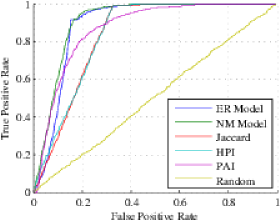
Figure 3: ROC curve of different algorithms on the Brightkite graph data

As Fig. 3 shows, the ROC curve of the algorithm that gives random scores is roughly a straight line from the origin to the top right corner. This line indicates that the algorithm cannot distinguish between an outlier edge and a normal edge, which is expected. The ROC curve of an algorithm that can detect outlier edges should be a curve above this straight line, as all algorithms used in this experiment. As mentioned in Section 3.2, the Jaccard Index and HPI both use the number of common neighbors. Thus their scores are all 0 for edges that connect two end nodes that do not share any common neighbors. In real-world graphs, a large amount of edges have a Jaccard Index or HPI value 0, especially for graphs that contain many low degree nodes.

The PAI value is the product of the degrees of the two end nodes of an edge. Sorting edges with their PAI values just puts the edges with low degree end nodes to the front. The figure shows that the PAI value can detect outlier edges with fairly good performance. This indicates that most of the injected edges connecting the nodes with low degrees. Considering most of the nodes in a real-world graph are low degree nodes, this is an expected behavior.

Fig. 3 indicates that the proposed outlier edge detection algorithms are clearly superior to the competing algorithms. The algorithm based on the PA model performs better than the one based on the ER model .

Table III shows the AUC values of the ROC curves on all test graph data. Bold font shows the best AUC values for each test graph.

TABLE III: AUC values of the ROC Curves on Different Graph Data

	ER	PA	Jaccard	HPI	PAI
advogato	0.887	0.893	0.858	0.859	0.877
twitter-icwsm	0.531	0.942	0.527	0.530	0.997
brightkite	0.885	0.905	0.833	0.827	0.873
facebook-wosn	0.968	0.970	0.947	0.946	0.878
ca-cit-HepPh	0.970	0.967	0.993	0.991	0.888
youtube-friend	0.770	0.842	0.731	0.738	0.898
web-Google	0.985	0.992	0.944	0.945	0.859

The comparison results show that the PA model algorithm gives consistently good performance regardless of the test graph data. The experiment also shows the correlation between the performance of the algorithms that are based on the random graph generation model and the GCC value of the test graph. For example, the ER model and PA model algorithms works better on Facebook-Wosn and Brightkite graph data, which have high GCC values as shown in Table II. Performance of the ER model algorithm degrades considerably on graphs with a very low GCC value, such as the twitter-icwsm graph. This result agrees with the fact that both the ER model and the PA model algorithms use the clustering property of graphs. We also observe that PAI works better on graphs with low GCC values. We estimate that these graphs contain many star structures and two nodes with low degrees are rarely linked by an edge. The large number of claw count (28 billion) and small number of triangle count (38k) in twitter-icwsm graph data partially confirm our estimation.

4.3 Change of Graph Properties

The proposed outlier edge detection algorithms are based on the clustering property of graphs. Since outlier edges are defined as edges that do not follow the clustering property, removing them should increase the coefficients that measure this property. On the other hand, some outlier edges (also called weak links in this aspect) serves an important role to connect remote nodes or nodes from different communities. Removing such edges should also extensively increase the distance of the two end nodes. Thus the coefficients that measure the distance between the nodes of a graph shall increase when outlier edges are removed. In this experiment, we verify these changes caused by the removal of the detected outlier edges.

The global clustering coefficient (GCC) and the average local clustering coefficient (ALCC) are the de facto measures of the clustering property of graphs. GCC is defined in Section 4.2. Local clustering coefficient (LCC) is the ratio of the number of edges that connect neighboring nodes of a node and the number of all possible edges that connect these neighboring nodes. The LCC of node $a$ can be expressed as

$$c_{a}=\frac{\left|\left\{\overline{ij}|i\in N_{a},j\in N_{a},\overline{ij}\in E\right\}\right|}{k_{a}\left(k_{a}-1\right)}.$$ (29)

ALCC is the average of the local clustering coefficients of all nodes in the graph.

We use diameter, the 90-percentile effective diameter (ED) and the mean shortest path (MSP) length as distance measures between the nodes in a graph. Diameter is the maximum shortest path length between any two nodes in a graph. 90-percentile effective diameter is the number of edges that are needed on average to reach 90% of other nodes. The mean shortest path length is the average of the shortest path length between each pair of nodes in the graph. Note, if the graph is not connected, we measure the diameter, ED and MSP of the largest component in the graph.

In this experiment, we removed 5% of the edges with the lowest outlier score. Table IV shows the GCC, ALCC, Diameter, ED and MSP values before and after the outlier edges were removed. For comparison, we also calculated values of these coefficients after same amount of edges are randomly removed 5% from the graph.

TABLE IV: Graph Properties Changes After Noise Edges Removal

	Original	ER Model	PA Model	Random
GCC	0.111	0.121	0.120	0.105
ALCC	0.172	0.180	0.183	0.158
Diameter	18	19	20	18
ED	5.91	6.78	6.36	5.95
MSP	3.92	4.10	4.10	3.95

The results show that removing the detected outlier edges clearly increases the GCC and ALCC values, while random edge removal slightly decreases the values. This confirms the enhancement of the clustering property after outlier edges are removed. The diameter, ED and MSP values all increase when the detected outlier edges were removed. This increase is much more significant than when random edges were removed. This also confirms the theoretical prediction.

5 Applications

In this section, we demonstrate various applications that benefit from the proposed outlier edge detection algorithms. In these applications, we use the algorithm of the PA model combined with scheme 4 and the score function defined by Eq. 23.

5.1 Impact on Graph Clustering Algorithms

Graph clustering is an important task in graph mining [29, 30, 31]. It aims to find clusters in a graph–a group of nodes in which the number of inner links between the nodes inside the group is much higher than that between the nodes inside the group and those outside the group. Many techniques have been proposed to solve this problem [32, 33, 34, 35].

The proposed outlier edge detection algorithms are based on the graph clustering property. They find edges that link the nodes in different clusters. These edges are also called weak links in the literature. With the proposed techniques, we can now remove detected outlier edges before applying a graph clustering algorithm. This should improve the graph clustering accuracy and reduce the computational time.

In this application, we evaluate the performance impact of the proposed outlier edge detection technique on different graph clustering algorithms. We use simulated graph data with cluster structures as used in [34, 36, 37, 38]. We generated test graphs of 512 nodes. The average degree of each node is 24. The generated cluster size varies from 16 to 256. Let $d_{out}$ be the average number of edges that link a node from the cluster to nodes outside the cluster. Let $d$ be the average degree of the node. Let $\mu=\frac{d_{out}}{d}$ be the parameter that indicates the strength of the clustering structure. The smaller $\mu$ is, the stronger the clustering structure is in the graph. We varied $\mu$ from 0.2 to 0.5. Note, when $\mu=0.5$, the graph has a very weak clustering structure, i.e. a node inside the cluster has an equal number of edges that link it to other nodes inside and outside the cluster.

We use the Normalized Mutual Information (NMI) to evaluated the accuracy of a graph clustering algorithm. The NMI value is between 0 and 1. The larger the NMI value is, the more accurate the graph clustering result is. An NMI value of 1 indicates that the clustering result matches the ground truth. More details of the NMI metric can be found in [33, 39].

We first apply graph clustering algorithms to the test graph data and record their NMI values and computational time. Then we remove 5% of the detected outlier edges from the test graph data, and apply these graph clustering algorithms again to the new graph and record their NMI values and computational time. The differences of the NMI values and the computational time show the impact of the outlier edge removal on the graph clustering algorithms.

The evaluated algorithms are GN [34], SLM [40], Danon [36], Louvain [32] and Infomap [41]. MCL [42] is not listed since it failed to find the cluster structure from this type of test graph data.

We repeated the experiment 10 times and calculated the average performance. Table V shows the NMI values before and after outlier edges were removed. The first number in each cell shows the NMI values of the clustering result on the original graph and the second number shows the NMI values of the clustering result on the graph after the outlier edges were removed.

TABLE V: The NMI Values Before and After Outlier Edges Were Removed

$\mu$	GN	SLM	Danon	Louvain	Infomap
0.2	0.99/1.0	1.0/1.0	0.99/1.0	1.0/1.0	1.0/1.0
0.25	0.98/0.99	1.0/1.0	0.99/0.98	1.0/1.0	1.0/1.0
0.3	0.93/0.97	1.0/1.0	0.95/0.98	1.0/1.0	0.92/1.0
0.35	0.74/0.72	0.96/0.94	0.66/0.84	0.90/0.86	0.36/0.91
0.4	0.66/0.70	0.83/0.81	0.67/0.70	0.84/0.81	0.78/0.83
0.45	0.53/0.52	0.71/0.67	0.51/0.55	0.68/0.60	0.22/0.43
0.5	0.39/0.47	0.58/0.56	0.39/0.49	0.51/0.53	0/0.47

Table VI shows the NMI value changes in percentage. A positive value indicates that the NMI value has increased.

TABLE VI: Changes of Normalized Mutual Information on Graph Clustering Algorithms in percentage

$\mu$	GN	SLM	Danon	Louvain	Infomap
0.2	0.8%	0	1.0%	0	0
0.25	1.5%	0	-1.0%	0	0
0.3	5.0%	0	3.5%	0	9.1%
0.35	-2.2%	-2.1%	26%	-4.9%	155%
0.4	6.7%	-2.2%	4.8%	-3.0%	5.8%
0.45	-1.1%	-6.2%	8.4%	-12%	95%
0.5	19%	-4.4%	26%	2.4%	$\infty$

The results show that outlier edge removal improves the accuracy of most graph clustering algorithms. The clustering accuracy of the SLM algorithm and the Louvain algorithm decrease slightly in some cases.

Table VII shows the computational time changes in percentage before and after outlier edges are removed. Negative values indicate that the computational time is decreased.

TABLE VII: Changes of Computational Time on Graph Clustering Algorithms in percentage

$\mu$	GN	SLM	Danon	Louvain	Infomap
0.2	-11%	-36%	-3.1%	-33%	-47%
0.25	-18%	1.0%	-1.0%	-41%	-16%
0.3	-9.3%	7.7%	-1.4%	-31%	-13%
0.35	-0.3%	-21%	-3.5%	-35%	31%
0.4	-5.7%	-5.3%	-3.0%	-20%	17%
0.45	2.8%	-14.4%	2.1%	-41%	33%
0.5	-6.7%	-1.9%	-3.4%	-39%	55%

These results show that outlier edge removal decreases the computational time of most algorithms used in the experiment. In some cases, SLM and the Louvain algorithms show significant gains in computation time. Note further that the increase of the computational time in the Infomap algorithm leads to a crucial improvement of the clustering accuracy.

5.2 Outlier Node Detection in Social Network Graphs

As mentioned in Section 2, many algorithms have been proposed to detect outlier nodes in a graph. In this section we present a technique to detect outlier nodes using the proposed outlier edge detection algorithm.

In a social network service, if a user generates many links that do not follow the clustering property, we have good reasons to suspect that the user is a scammer. To detect this type of outlier nodes, we can first detect outlier edges. Then we find nodes that are the end points of these outlier edges. Nodes that are linked to many outlier edges are likely to be outlier nodes.

In this application, we use Brightkite data for outlier node detection. In the experiment, we rank the edges according to their outlier scores. We take the first 1000 edges as outlier edges and rank each node according to the number of outlier edges that it is connected to.

Table VIII shows the top 8 detected outlier nodes: the node ID, the number of outlier edges that the node links, the degree of the node, the rank of the degree among all nodes and LCC values of the node.

TABLE VIII: Outlier Node Detection Results on Brightkite Graph

node id	outlier edges	degree	degree rank	LCC
41	21	1134	1	0.005
458	16	1055	2	0.001
115	9	838	4	0.004
175	7	270	39	0.001
989	7	270	40	0.015
2443	7	379	16	0.010
36	5	467	11	0.005
158	5	833	5	0.004

The results show that the detected outlier nodes tend to have large degree values. In particular, the LCC values of the detected outlier nodes are extremely low comparing to the ALCC value (0.172) of the graph. This shows that the neighboring nodes of the detected outlier nodes have very weak clustering property.

5.3 Clustering of Noisy Data

Clustering is one of the most important tasks in machine learning [43]. During the last decades, many algorithms have been proposed, i.e. [44, 45, 46]. The task becomes more challenging when noise is present in the data. Many algorithms, especially connectivity-based clustering algorithms, fail over such data. In this section we present a robust clustering algorithm that uses the proposed outlier edge detection techniques to find correct clusters in noisy data.

Graph algorithms have been successfully used in clustering problems [47, 48]. To cluster the data, we first build a mutual $k$-nearest neighbor (MKNN) graph [49, 50]. Let $x_{1},x_{2},\ldots,x_{n}\in R^{d}$ be the data points, where $n$ is the number of data points and $d$ is the dimension of the data. Let $d(x_{i},x_{j})$ be the distance between two data points $x_{i}$ and $x_{j}$. Let $N_{k}(x_{i})$ be the set of data points that are the $k$-nearest neighbors of the data point $x_{i}$ with respect to the predefined distance measure $d\left(x_{i},x_{j}\right)$. Therefore, the cardinality of the set $N_{k}(x_{i})$ is $k$. A MKNN graph is built in the following way. The nodes in the MKNN graph are the data points. Two nodes $x_{i}$ and $x_{j}$ are connected if $x_{i}\in N_{k}(x_{j})$ and $x_{j}\in N_{k}(x_{i})$. The constructed MKNN graph is unweighted and undirected.

With a proper distance function, data points in a cluster are close to each other whereas data points in different clusters are far away from each other. Thus, in the constructed MKNN graph, a node is likely to be linked to other nodes in the same cluster while the links between the nodes in different clusters are relatively less. This indicates that the MKNN graph has the clustering property similar to social network graphs.

Outlier data points are normally far away from the normal data points. Some outlier nodes form isolated small components in the MKNN graph. However, the outlier nodes that fall between the clusters form bridges that connect different clusters. These bridges greatly degrade the performance of connectivity-based clustering algorithms, such as single-linkage clustering algorithm and complete-linkage clustering algorithm [43].

Based on these observations, we propose a hierarchical clustering algorithm by iteratively removing edges (weak links) according to their outlier scores. When a certain amount of outlier edges is removed, different clusters form separate large connected components–a connected component in a graph that contains a large proportion of the nodes, and it is straightforward to find them in the graph. A breadth-first search or a depth-first search algorithm can find all connected components in a graph with the complexity of $O(n)$, where $n$ is the number of nodes. At each iteration step, we find large connected components in the MKNN graph and the data points that do not belong to any large connected components are classified as outliers.

Using the proposed algorithm, we cluster a dataset taken from [51]. Fig. 4 shows some results of different number of detected clusters. Outliers are shown in light gray color and data points in different clusters are shown in different colors.

(a)	(b)
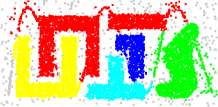
(c)	(d)
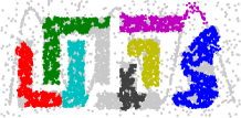
(e)	(f)

Figure 4: Clustering results of a dataset taken from [51]. (a) 1 cluster; (b) 2 clusters; (c) 4 clusters; (d) 5 clusters; (e) 6 clusters; (f) 7 clusters.

As the Fig. 4 shows, the proposed algorithm cannot only classify outliers and normal data points but also find clusters in the data points. As more and more edges are removed from the MKNN graph, the number of clusters increases.

Next we show how to determine the true number of clusters. Table IX shows the number of removed edges and the number of detected clusters of this dataset.

TABLE IX: Percentage of the Removed Edges and the Number of Detected Clusters

removed edges	2.6%	2.7%	2.8%	3.5%	6%	33.3%
number of clusters	2	3	4	5	6	7

As the result shows, removing a small amount of edges is enough to find correct clusters in the data. One has to remove a large amount of edges to break a genuine cluster into smaller components. We can simply define a threshold and stop the iteration if the number of clusters does not increase any more.

To illustrate the performance of the proposed clustering algorithm, we use synthetic data that are both noisy and challenging. Fig. 5 shows the test datasets. We used tools from [52] to generate the normal data points and added random data points as noise.

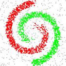
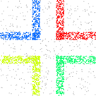
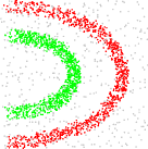
(a)	(b)	(c)
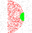
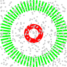
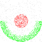
(d)	(e)	(f)

Figure 5: Synthetic datasets for clustering

In our experiments, we use the Euclidean distance function. The number of nearest neighbors is 30. At each iteration step, we remove 0.1% of total number of edges according to their outlier scores. A large connected component is a component whose size is larger than 5% of the total number of nodes. The clustering termination threshold is set as 10% of the total number of edges.

We compare the proposed clustering algorithm with the k-means[43], the average-linkage (a-link)[43], the normalized cuts (N-Cuts)[53] and the graph degree linkage (GDL)[46] clustering algorithms. Since the competing algorithms cannot detect the number of clusters, we use the value from the ground truth. Table X shows the NMI scores of the proposed algorithm and the competing algorithms.

TABLE X: Clustering of Noisy Data Results

dataset	k-means	a-link	N-Cuts	GDL	proposed
(a)	0.031	0.099	0.053	0.650	0.672
(b)	0.743	0.743	0.743	0.743	0.848
(c)	0	0.004	0.559	0.654	0.755
(d)	0.208	0.161	0.367	0.553	0.619
(e)	0.001	0.133	0.680	0.701	0.744
(f)	0.001	0.162	0.627	0.612	0.714

The results show that the k-means and the average linkage clustering algorithms fail on complex-shaped clusters. GDL and the proposed algorithms are all graph-based clustering algorithms. They are able to find clusters with arbitrary shapes. From the NMI scores, the proposed algorithm is clearly superior to the competing clustering algorithms.

6 Conclusions

In real-world graphs, in particular social network graphs, there are edges generated by scammers, malicious programs or mistakenly by normal users and the system. Detecting these outlier edges and removing them will not only improve the efficiency of graph mining and analytics, but also help identify harmful entities. In this article, we introduce outlier edge detection algorithms based on two random graph generation models. We define four schemes that represent relationships of two nodes and the groups of their neighboring nodes. We combine the schemes with the two random graph generation models and investigate the proposed algorithms theoretically. We tested the proposed outlier edge detection algorithms by experiments on real-world graphs. The experimental results show that our proposed algorithms can effectively identify the injected edges in real-world graphs. We compared the performance of our proposed algorithms with other outlier edge detection algorithms. The proposed algorithms, especially the algorithm based on the PA model, give consistently good results regardless of the test graph data. We also evaluated the changes of graph properties caused by the removal of the detected outlier edges. The experimental results show an increase in both the clustering coefficients and the increase of the distance between the nodes in the graph. This is coherent with the theoretical predictions.

Further more, we demonstrate the potential of the outlier edge detection using three different applications. When used with the graph clustering algorithms, removing outlier edges from the graph not only improves the clustering accuracy but also reduces the computational time. This indicates that the proposed algorithms are powerful preprocessing tools for graph mining. When used for detecting outlier nodes in social network graphs, we can successfully find outlier nodes whose behavior deviates dramatically from that of normal nodes. We also present a clustering algorithm that is based on the edge outlier scores. The clustering algorithm can efficiently find true data clusters by excluding noises from the data.

Outlier edge detection has great potentials in numerous Big Data applications. In the future, we will apply the proposed outlier edge detection algorithms in applications in other fields, for example computer vision and content-based multimedia retrieval in the Big Visual Data. We observed that nodes and edges outside edge-ego-network also contain valuable information in outlier detection. However, using this information dramatically increases the computational cost. We will work on fast algorithms that can efficiently use the structural information of the whole graph.

Proof of Theorem 4

Proposition 8.

$\alpha\left(S\cup T,R\right)=\alpha\left(S,R\right)+\alpha\left(T,R\right)$ if $S\cap T=\emptyset$.

Proof:

Let $A$ be the adjacency matrix of an unweighted and undirected graph $G$. We have $\alpha(S,T)=\sum_{i\in S}\sum_{j\in T}A_{ij}$. Given $S\cap T=\emptyset$,

$$\alpha\left(S\cup T,R\right) =\sum_{i\in S\cup T}\sum_{j\in R}A_{ij}$$

$$=\sum_{i\in S}\sum_{j\in R}A_{ij}+\sum_{i\in T}\sum_{j\in R}A_{ij}$$

$$=\alpha(S,R)+\alpha(T,R)$$

∎

Next we prove Theorem 4.

Proof:

For scheme 4, $P_{a,b}^{(4)}=S_{a\backslash b}$, $R_{a,b}^{(4)}=S_{b\backslash a}$, $P_{b,a}^{(4)}=S_{b\backslash a}$ and $R_{b,a}^{(4)}=S_{a\backslash b}$. Using Theorem 3, we can easily get $\alpha\left(P_{a,b}^{(4)},R_{a,b}^{(4)}\right)=\alpha\left(P_{b,a}^{(4)},R_{b,a}^{(4)}\right)$.

To prove Theorem 4 for scheme 2, we divide the nodes in edge-ego-network $G_{\overline{ab}}$ into five mutually exclusive sets:

• $V_{1}=\left\{x|x\in N_{a}\ \mathrm{and}\ x\notin S_{b}\right\}$;

• $V_{2}=\left\{x|x\in N_{b}\ \mathrm{and}\ x\notin S_{a}\right\}$;

• $V_{3}=\left\{x|x\in N_{a}\ \mathrm{and}\ x\in N_{b}\right\}$;

• $V_{4}=\left\{a\right\}$;

• $V_{5}=\left\{b\right\}$.

From the definition, we have

$$P_{a,b}^{(2)} =N_{a\backslash b}=V_{1}\cup V_{3},$$

$$R_{a,b}^{(2)} =S_{b\backslash a}=V_{2}\cup V_{3}\cup V_{5},$$

$$P_{b,a}^{(2)} =N_{b\backslash a}=V_{2}\cup V_{3},$$

$$R_{b,a}^{(2)} =S_{a\backslash b}=V_{1}\cup V_{3}\cup V_{4}.$$

Using the definition of $\alpha(S,T)$ and Proposition 8, we get

$$\alpha\left(P_{a,b}^{(2)},R_{a,b}^{(2)}\right) = \alpha\left(V_{1}\cup V_{3},V_{2}\cup V_{3}\cup V_{5}\right)$$

$$= \alpha\left(V_{1},V_{2}\right)+\alpha\left(V_{1},V_{3}\right)+\alpha\left(V_{1},V_{5}\right)$$

$$+\alpha\left(V_{3},V_{2}\right)+\alpha\left(V_{3},V_{3}\right)+\alpha\left(V_{3},V_{5}\right)$$

and

$$\alpha\left(P_{b,a}^{(2)},R_{b,a}^{(2)}\right) = \alpha\left(V_{2}\cup V_{3},V_{1}\cup V_{3}\cup V_{4}\right)$$

$$= \alpha\left(V_{2},V_{1}\right)+\alpha\left(V_{2},V_{3}\right)+\alpha\left(V_{2},V_{4}\right)$$

$$+\alpha\left(V_{3},V_{1}\right)+\alpha\left(V_{3},V_{3}\right)+\alpha\left(V_{3},V_{4}\right)$$

Taking the fact that $\alpha(V_{1}\cap V_{5})=0$, $\alpha(V_{2}\cap V_{4})=0$, and $\alpha(V_{3},V_{4})=\alpha(V_{3},V_{5})$, the right hand side of Eqs. Proof: and Proof: are equal. Thus $\alpha\left(P_{a,b}^{(2)},R_{a,b}^{(2)}\right)=\alpha\left(P_{b,a}^{(2)},R_{b,a}^{(2)}\right)$. ∎

Honglei Zhang is a PhD student and a researcher in the Department of Signal Processing at Tampere University of Technology. He received his Bachelor and Master degree in Electrical Engineering from Harbin Institute of Technology in 1994 and 1996 in China, respectively. He worked as a software engineer in Founder Co. in China from 1996 to 1999. He had been working as a software engineer and a software system architect in Nokia Oy Finland for 14 years. He has 6 scientific publications and 2 patents. His current research interests include computer vision, pattern recognition, data mining and graph algorithms. More about of his research can be found from http://www.cs.tut.fi/~zhangh.

Serkan Kiranyaz was born in Turkey, 1972. He received his BS degree in Electrical and Electronics Department at Bilkent University, Ankara, Turkey, in 1994 and MS degree in Signal and Video Processing from the same University, in 1996. He worked as a Senior Researcher in Nokia Research Center and later in Nokia Mobile Phones, Tampere, Finland. He received his PhD degree in 2005 and his Docency at 2007 from Tampere University of Technology, respectively. He is currently a Professor in the Department of Electrical Engineering at Qatar University. Prof. Kiranyaz published 2 books, more than 30 journal papers in several IEEE Transactions and some other high impact journals and 70+ papers in international conferences. His recent publication has been nominated for the Best Paper Award in IEEE ICIP’13 conference. Another publication won the IBM Best Paper Award in ICPR’14.

Moncef Gabbouj received his BS degree in electrical engineering in 1985 from Oklahoma State University, and his MS and PhD degrees in electrical engineering from Purdue University, in 1986 and 1989, respectively. Dr. Gabbouj is currently Academy of Finland Professor and holds a permanent position of Professor of Signal Processing at the Department of Signal Processing, Tampere University of Technology. His research interests include multimedia content-based analysis, indexing and retrieval, machine learning, nonlinear signal and image processing and analysis, voice conversion, and video processing and coding. Dr. Gabbouj is a Fellow of the IEEE and member of the Finnish Academy of Science and Letters. He is the past Chairman of the IEEE CAS TC on DSP and committee member of the IEEE Fourier Award for Signal Processing. He served as Distinguished Lecturer for the IEEE CASS. He served as associate editor and guest editor of many IEEE, and international journals.

References

- [1] M. Newman, Networks: An Introduction, 1st ed. Oxford ; New York: Oxford University Press, May 2010.
- [2] M. Jiang, P. Cui, A. Beutel, C. Faloutsos, and S. Yang, “CatchSync: Catching Synchronized Behavior in Large Directed Graphs,” in Proceedings of the 20th ACM SIGKDD International Conference on Knowledge Discovery and Data Mining, ser. KDD ’14. New York, NY, USA: ACM, 2014, pp. 941–950.
- [3] A. Beutel, W. Xu, V. Guruswami, C. Palow, and C. Faloutsos, “CopyCatch: stopping group attacks by spotting lockstep behavior in social networks,” in Proceedings of the 22nd international conference on World Wide Web. International World Wide Web Conferences Steering Committee, 2013, pp. 119–130.
- [4] L. Akoglu, H. Tong, and D. Koutra, “Graph based anomaly detection and description: a survey,” Data Mining and Knowledge Discovery, pp. 1–63, 2014.
- [5] C. C. Noble and D. J. Cook, “Graph-based anomaly detection,” in Proceedings of the ninth ACM SIGKDD international conference on Knowledge discovery and data mining. ACM, 2003, pp. 631–636.
- [6] H. Dai, F. Zhu, E. P. LIM, and H. H. PANG, “Detecting anomalies in bipartite graphs with mutual dependency principles.” The 12th IEEE International Conference on Data Mining (ICDM’12), 2012.
- [7] K. Henderson, B. Gallagher, T. Eliassi-Rad, H. Tong, S. Basu, L. Akoglu, D. Koutra, C. Faloutsos, and L. Li, “Rolx: structural role extraction & mining in large graphs,” in Proceedings of the 18th ACM SIGKDD international conference on Knowledge discovery and data mining. ACM, 2012, pp. 1231–1239.
- [8] V. J. Hodge and J. Austin, “A Survey of Outlier Detection Methodologies,” Artificial Intelligence Review, vol. 22, no. 2, pp. 85–126, Oct. 2004.
- [9] X. Xu, N. Yuruk, Z. Feng, and T. A. J. Schweiger, “SCAN: A Structural Clustering Algorithm for Networks,” in Proceedings of the 13th ACM SIGKDD International Conference on Knowledge Discovery and Data Mining, ser. KDD ’07. New York, NY, USA: ACM, 2007, pp. 824–833.
- [10] J. Gao, F. Liang, W. Fan, C. Wang, Y. Sun, and J. Han, “On Community Outliers and Their Efficient Detection in Information Networks,” in Proceedings of the 16th ACM SIGKDD International Conference on Knowledge Discovery and Data Mining, ser. KDD ’10. New York, NY, USA: ACM, 2010, pp. 813–822.
- [11] L. Akoglu, M. McGlohon, and C. Faloutsos, “oddball: Spotting Anomalies in Weighted Graphs,” in Advances in Knowledge Discovery and Data Mining, ser. Lecture Notes in Computer Science, M. J. Zaki, J. X. Yu, B. Ravindran, and V. Pudi, Eds. Springer Berlin Heidelberg, 2010, no. 6119, pp. 410–421.
- [12] D. Chakrabarti, “AutoPart: Parameter-Free Graph Partitioning and Outlier Detection,” in Knowledge Discovery in Databases: PKDD 2004, ser. Lecture Notes in Computer Science, J.-F. Boulicaut, F. Esposito, F. Giannotti, and D. Pedreschi, Eds. Springer Berlin Heidelberg, 2004, no. 3202, pp. 112–124.
- [13] D. Easley and J. Kleinberg, Networks, crowds, and markets. Cambridge Univ Press, 2012.
- [14] L. Lü and T. Zhou, “Link prediction in complex networks: A survey,” Physica A: Statistical Mechanics and its Applications, vol. 390, no. 6, pp. 1150–1170, Mar. 2011.
- [15] N. Barbieri, F. Bonchi, and G. Manco, “Who to Follow and Why: Link Prediction with Explanations,” in Proceedings of the 20th ACM SIGKDD International Conference on Knowledge Discovery and Data Mining, ser. KDD ’14. New York, NY, USA: ACM, 2014, pp. 1266–1275.
- [16] L. C. Freeman, “Centered graphs and the structure of ego networks,” Mathematical Social Sciences, vol. 3, no. 3, pp. 291–304, 1982.
- [17] D. J. Watts and S. H. Strogatz, “Collective dynamics of ‘small-world’networks,” nature, vol. 393, no. 6684, pp. 440–442, 1998.
- [18] M. Coscia, G. Rossetti, F. Giannotti, and D. Pedreschi, “DEMON: A Local-first Discovery Method for Overlapping Communities,” in Proceedings of the 18th ACM SIGKDD International Conference on Knowledge Discovery and Data Mining, ser. KDD ’12. New York, NY, USA: ACM, 2012, pp. 615–623.
- [19] B. Bollobás, Random Graphs, 2nd ed. Cambridge ; New York: Cambridge University Press, Oct. 2001.
- [20] M. E. J. Newman, “Modularity and community structure in networks,” Proceedings of the National Academy of Sciences, vol. 103, no. 23, pp. 8577–8582, Jun. 2006.
- [21] E. Cho, S. A. Myers, and J. Leskovec, “Friendship and Mobility: User Movement in Location-based Social Networks,” in Proceedings of the 17th ACM SIGKDD International Conference on Knowledge Discovery and Data Mining, ser. KDD ’11. New York, NY, USA: ACM, 2011, pp. 1082–1090.
- [22] J. Kunegis, “KONECT – The Koblenz Network Collection,” in Proc. Int. Conf. on World Wide Web Companion, 2013, pp. 1343–1350.
- [23] P. Massa, M. Salvetti, and D. Tomasoni, “Bowling alone and trust decline in social network sites,” in Dependable, Autonomic and Secure Computing, 2009. DASC’09. Eighth IEEE International Conference on. IEEE, 2009, pp. 658–663.
- [24] M. De Choudhury, Y.-R. Lin, H. Sundaram, K. S. Candan, L. Xie, and A. Kelliher, “How does the data sampling strategy impact the discovery of information diffusion in social media?” ICWSM, vol. 10, pp. 34–41, 2010.
- [25] B. Viswanath, A. Mislove, M. Cha, and K. P. Gummadi, “On the evolution of user interaction in facebook,” in Proceedings of the 2nd ACM workshop on Online social networks. ACM, 2009, pp. 37–42.
- [26] J. Leskovec, J. Kleinberg, and C. Faloutsos, “Graph evolution: Densification and shrinking diameters,” ACM Transactions on Knowledge Discovery from Data (TKDD), vol. 1, no. 1, p. 2, 2007.
- [27] J. Yang and J. Leskovec, “Defining and evaluating network communities based on ground-truth,” Knowledge and Information Systems, vol. 42, no. 1, pp. 181–213, 2015.
- [28] J. Leskovec, K. J. Lang, A. Dasgupta, and M. W. Mahoney, “Statistical properties of community structure in large social and information networks,” in Proceedings of the 17th international conference on World Wide Web. ACM, 2008, pp. 695–704.
- [29] S. Fortunato, “Community detection in graphs,” Physics Reports, vol. 486, no. 3–5, pp. 75–174, Feb. 2010.
- [30] M. Coscia, F. Giannotti, and D. Pedreschi, “A classification for community discovery methods in complex networks,” Statistical Analysis and Data Mining, vol. 4, no. 5, pp. 512–546, Oct. 2011.
- [31] S. Papadopoulos, Y. Kompatsiaris, A. Vakali, and P. Spyridonos, “Community detection in Social Media,” Data Mining and Knowledge Discovery, vol. 24, no. 3, pp. 515–554, Jun. 2011.
- [32] V. D. Blondel, J.-L. Guillaume, R. Lambiotte, and E. Lefebvre, “Fast unfolding of communities in large networks,” Journal of Statistical Mechanics: Theory and Experiment, vol. 2008, no. 10, p. P10008, 2008.
- [33] L. Danon, A. Diaz-Guilera, J. Duch, and A. Arenas, “Comparing community structure identification,” Journal of Statistical Mechanics: Theory and Experiment, vol. 2005, no. 09, p. P09008, 2005.
- [34] M. E. Newman and M. Girvan, “Finding and evaluating community structure in networks,” Physical review E, vol. 69, no. 2, p. 026113, 2004.
- [35] S. E. Schaeffer, “Graph clustering,” Computer Science Review, vol. 1, no. 1, pp. 27–64, 2007.
- [36] L. Danon, A. Díaz-Guilera, and A. Arenas, “The effect of size heterogeneity on community identification in complex networks,” Journal of Statistical Mechanics: Theory and Experiment, vol. 2006, no. 11, p. P11010, Nov. 2006.
- [37] A. Lancichinetti, S. Fortunato, and F. Radicchi, “Benchmark graphs for testing community detection algorithms,” Physical Review E, vol. 78, no. 4, Oct. 2008.
- [38] M. E. Newman, “Fast algorithm for detecting community structure in networks,” Physical review E, vol. 69, no. 6, p. 066133, 2004.
- [39] L. Ana and A. Jain, “Robust data clustering,” in 2003 IEEE Computer Society Conference on Computer Vision and Pattern Recognition, 2003. Proceedings, vol. 2, Jun. 2003, pp. II–128–II–133 vol.2.
- [40] L. Waltman and N. J. v. Eck, “A smart local moving algorithm for large-scale modularity-based community detection,” The European Physical Journal B, vol. 86, no. 11, pp. 1–14, Nov. 2013.
- [41] M. Rosvall and C. T. Bergstrom, “Maps of random walks on complex networks reveal community structure,” Proceedings of the National Academy of Sciences, vol. 105, no. 4, pp. 1118–1123, Jan. 2008.
- [42] S. Dongen, “Graph clustering by flow simulation,” Ph.D. dissertation, Universiteit Utrecht, Utrecht, The Netherlands, May 2000.
- [43] S. Theodoridis and K. Koutroumbas, Pattern Recognition, Fourth Edition, 4th ed. Amsterdam: Academic Press, Nov. 2008.
- [44] A. K. Jain, M. N. Murty, and P. J. Flynn, “Data clustering: a review,” ACM computing surveys (CSUR), vol. 31, no. 3, pp. 264–323, 1999.
- [45] S. Lloyd, “Least squares quantization in PCM,” IEEE Transactions on Information Theory, vol. 28, no. 2, pp. 129–137, Mar. 1982.
- [46] W. Zhang, X. Wang, D. Zhao, and X. Tang, “Graph Degree Linkage: Agglomerative Clustering on a Directed Graph,” in Computer Vision – ECCV 2012, ser. Lecture Notes in Computer Science, A. Fitzgibbon, S. Lazebnik, P. Perona, Y. Sato, and C. Schmid, Eds. Springer Berlin Heidelberg, 2012, no. 7572, pp. 428–441.
- [47] D. Harel and Y. Koren, “On Clustering Using Random Walks,” in FST TCS 2001: Foundations of Software Technology and Theoretical Computer Science, ser. Lecture Notes in Computer Science, R. Hariharan, V. Vinay, and M. Mukund, Eds. Springer Berlin Heidelberg, 2001, no. 2245, pp. 18–41.
- [48] X. Dong, P. Frossard, P. Vandergheynst, and N. Nefedov, “Clustering With Multi-Layer Graphs: A Spectral Perspective,” IEEE Transactions on Signal Processing, vol. 60, no. 11, pp. 5820–5831, Nov. 2012.
- [49] M. R. Brito, E. L. Chávez, A. J. Quiroz, and J. E. Yukich, “Connectivity of the mutual k-nearest-neighbor graph in clustering and outlier detection,” Statistics & Probability Letters, vol. 35, no. 1, pp. 33–42, Aug. 1997.
- [50] K. Ozaki, M. Shimbo, M. Komachi, and Y. Matsumoto, “Using the mutual k-nearest neighbor graphs for semi-supervised classification of natural language data,” in Proceedings of the Fifteenth Conference on Computational Natural Language Learning. Association for Computational Linguistics, 2011, pp. 154–162.
- [51] G. Karypis, E.-H. Han, and V. Kumar, “Chameleon: Hierarchical clustering using dynamic modeling,” Computer, vol. 32, no. 8, pp. 68–75, 1999.
- [52] “6 functions for generating artificial datasets - File Exchange - MATLAB Central.”
- [53] J. Shi and J. Malik, “Normalized cuts and image segmentation,” Pattern Analysis and Machine Intelligence, IEEE Transactions on, vol. 22, no. 8, pp. 888–905, 2000.