Compact Galactic Planetary Nebulae: A HST/WFC3 Morphological Catalog, and a Study of their Role in the Galaxy

Abstract

We present the images of a Hubble Space Telescope (HST/WFC3) snapshot program of angularly compact Galactic planetary nebulae (PNe), acquired with the aim of studying their size, evolutionary status, and morphology. PNe that are smaller than $\sim 4\arcsec$ are underrepresented in most morphological studies, and today they are less well studied than their immediate evolutionary predecessors, the pre-planetary nebulae. The images have been acquired in the light of [O III]$\lambda 5007$, which is commonly used to classify the PN morphology, in the UV continuum with the aim of detecting the central star unambiguously, and in the $I-$band to detect a cool stellar companion, if present. The sample of 51 confirmed PNe exhibits nearly the full range of primary morphological classes, with the distribution more heavily weighted toward bipolar PNe, but with total of aspherical PNe almost identical to that of the general Galactic sample. A large range of microstructures is evident in our sample as well, with many nebulae displaying attached shells, halos, ansae, and internal structure in the form of arcs, rings, and spirals. Various aspherical structures in a few PNe, including detached arcs, suggest an interaction with the ISM. We studied the observed sample of compact Galactic PNe in the context of the general Galactic PN population, and explore whether their physical size, spatial distribution, reddening, radial metallicity gradient, and possible progenitors, are peculiar within the population of Galactic PNe. We found that these compact Galactic PNe, which have been selected based on apparent dimensions, constitute a diverse Galactic PN population that is relatively uniformly distributed across the Galactic disk, including the outskirts of our Galaxy. This unique sample will be used in the future to probe the old Galactic disk population.

1 Introduction

Planetary nebulae (PNe) are ionized shells of gas that were ejected by Asymptotic Giant Branch (AGB) stars at the end of their evolution. The ejection symmetry, slow expansion rate, rapidly evolving central star (CS) that may feature a fast wind and magnetic fields, presence of interstellar medium materials, dust content, and central star multiplicity produce PNe with a variety of shapes that may change during their short, hydrodynamical evolution. In the Galaxy, studies based on PN image catalogs (e.g., Schwarz et al., 1992; Manchado et al., 1996) have shown that PN projected macro-morphologies can be usefully grouped into a few basic classes, and that round (R), elliptical (E), bipolar core (BC), and bipolar (B) shapes are the most commonly observed. Morphology is best studied with narrow-band imagery, and typically gives a reasonable classification for all PNe that are larger than $\sim 4\arcsec$ to obtain a well spatially-resolved PN image as observed with ground-based telescopes. This empirical limitation is due to the minimum number of resolution elements needed to sensibly determine morphology. For this reason, Galactic morphological catalogs cannot classify the angularly small PNe, which are then labelled unresolved or point-source.

With HST cameras it has become possible to determine the morphology of spatially compact PNe. In the past decades HST has revealed the shape and apparent size of extragalactic PNe such as those in the Large and Small Magellanic Clouds (e.g., Stanghellini et al. 2000, 2003; Shaw et al. 2001, 2006), which are almost invariably unresolved from the ground, and whose apparent diameters are typically $\sim 0.5\arcsec$. On the other hand, compact Galactic PNe, with apparent radius $<4\arcsec$, have not been studied as an independent group to date, but several such objects have corresponding HST images (e.g., Hsia et al., 2014) that reveal their shapes. Compact Galactic PNe are important for a variety of reasons: as a group, they may be predominantly farther away than other Galactic PNe, or they may be younger – recently ejected – with respect to the general population. In the former case, this sample gives the chance to peer farther into the Galactic disk when using PNe as probes of Galactic structure and evolution, while in the latter case it gives a chance to study early PN morphology, soon after the ionization onset. Only by studying a sizable sample of compact PNe we would be able to disclose their original stellar population and evolutionary stage.

Compact PNe offer another advantage with respect to the general population: their spectra, both optical and IR, can be acquired with just one pointing to include the whole nebula, which in turns provides plasma diagnostics and chemical analysis of the PN as a whole. This is important for ground-based optical spectroscopy, and even more so for mid-IR space spectroscopy. For example, their compact shapes allowed the study of dust content with Spitzer/IRS spectroscopy; dust analysis of more than 150 compact Galactic PNe is available to date (Stanghellini et al. 2012). Dust plays an important role in PN formation, where radiation pressure on dust grains causes stellar winds, and thus must affect PN shaping. By studying Magellanic Cloud PNe, it has been shown that dust type and morphology are correlated (Stanghellini et al., 2007).

In this paper we present a morphological catalog of compact Galactic PNe observed with HST/WFC3. This is the largest bf homogeneous sample of compact Galactic PNe observed to date. The observations made it possible to determine the PN apparent radii, their morphology, and to study their CSs. Here we present the nebular aspect of this sample, while the CS analysis, including that of possible companion stars, will be published in Moreno-Ibáñez et al. (2016) and elsewhere.

In Section 2 we describe the observations that yielded to 51 PNe images in 3 filters. In $\S$ 3 we give the photometric radii, fluxes, and classification of individual morphology, measured from the images, and a discussion on their distances and physical sizes. Section 4 includes a discussion on the relation between morphology and dust types of compact PNe. In $\S$ 5 we compare compact PNe with the general Galactic PN population. This includes comparing physical dimensions, morphology, dust type, Galactic distribution, and radial metallicity gradients. Section 6 includes a discussion of our findings. Finally, $\S 7$ gives the conclusions, and some directions for potential future research.

2 Observations

The goal of our HST snapshot program (GO 11657; PI: L. Stanghellini) was to obtain high-resolution images of a substantial sample of angularly small PNe (i.e., with published angular diameters $<4\arcsec$) whose ground-based observations are insufficient both to determine nebular morphology with adequate detail, and to measure CS fluxes against the bright nebular emission. The target selection for this program includes all known compact Galactic PNe. The population of spectroscopically confirmed Galactic PNe is described in the Strasbourg-ESO catalog of Galactic PNe (Acker et al., 1992), and in the MASH survey (Parker et al., 2006). Of the 1143 PNe listed by Acker et al. (1992), 143 are point-sources and 86 have ground-based measured radii $\theta<4\arcsec$. The MASH survey adds two compact PNe with $\theta<4\arcsec$, but no point sources. From these compact targets we explicitly removed all Galactic Bulge and Halo PNe, to obtain a pure Galactic disk population of compact PNe. To assess whether a PN belongs to the Galactic bulge or halo we used the criteria defined by Stanghellini & Haywood (2010, hereafter SH10) but more precise population assessment, which is based also on their distance, can be done only a posteriori for compact PNe, once their statistical distances can be reliably calculated from their photometric radii.

From the target sample we excluded those PNe that have been previously observed with HST WFPC2 and ACS in similar imaging modes to avoid duplications. We did not however exclude PNe already observed with pre-COSTAR HST imaging, since the PN dimensions obtained from these images are not reliable (Stanghellini et al. 2000). By proposing these observations in snapshot mode we further reduced the target list by only including targets that are bright enough the be observed within one orbit. Our approved program consisted of 130 targets.

Observations of compact Galactic PNe were acquired with HST Wide-Field Camera 3 (Kimble et al., 2008) through four filters. We used F502N to obtain images of the targets in the light of [O III] $\lambda 5007$, which is very often among the brightest emission lines in PNe, and it is customary used to classify the morphology and measure the angular dimensions with aperture photometry. We also imaged each target with F200LP, which passes essentially all wavelengths to which the detectors are sensitive, and in particular takes advantage of the extraordinary sensitivity of this camera to near-UV light (Dressel et al., 2010). We complemented the NUV exposures with F350LP, which blocks UV light but passes all visible light; the difference between the calibrated flux of the CS in F200LP and that in F350LP yields a UV continuum magnitude. Finally, we imaged each target with F814W to measure the stellar the $I-$band continuum. All images except those in F814W were split into sub-exposure pairs to enable cosmic-ray rejection. Images in the UV and IR continuum allowed measuring the magnitude and color of the CS (Moreno-Ibáñez et al., 2016).

We planned our exposure durations in F502N to yield an average signal-to-noise ratio (S/N) of at least 16 pixel^-1, based on the $H\beta$ fluxes of Acker et al. (1991), and the $I(5007)/I(H\beta)$ relative intensities and angular diameters as compiled by Acker et al. (1992). For objects with no published [O III] flux we assumed $I(5007)=I(H\alpha)$ at zero reddening. Our experience with prior HST programs indicates that images so exposed yield useful morphological detail. We note that the substantial error in the published angular diameters (which are all taken from ground-based observations) yielded large uncertainties in the estimated exposure times. Our estimates of the optimal exposure durations for the continuum filters was more uncertain still, since we had no information on the CS magnitudes. The absolute brightness of a CS can vary by 10 mag in $V$ as it evolves at nearly constant luminosity from 30,000 K to well over 100,000 K, before fading to the white dwarf cooling track. In the end we planned the F200LP and F350LP exposures to yield a S/N of $\sim 20$ for a star with apparent magnitude $V=25$ and a temperature of $10^{5}$ K. We added a second exposure in these filters that was usually shorter by a factor of a few to 10. This combination of exposures allowed sufficient dynamic range to minimize the risk of saturation for bright, nearby CSs while providing useful S/N for faint, distant stars. For F814W we planned a single exposure, modified for interstellar extinction, that would yield useful S/N for a possible companion between types G2V and M5V.

Minimizing visit duration without compromising science is always a key concern for HST snapshot programs. Our strategy was to reduce the detector read-out time by using sub-array apertures, which allows all the exposures during a visit to be stored in the instrument memory, rather than incurring the overhead of a buffer dump to external storage. For F502N it was important to image the entire nebula (which could have structure larger than the nominal 4″), and to allow for the possibility of errors in the coordinates, which were taken from Kerber et al. (2003). We therefore used the UVIS1-2K4-SUB aperture, which covers a roughly 2K $\times$ 4K pixel (82″$\times$164″) field of view using CCD1. The continuum exposures used the UVIS1-C512A-SUB aperture which covers a $512\times 512$ pixel ($20\arcsec\times 20\arcsec$) sub-array located in the corner of CCD 1, near a read-out amplifier. This approach minimizes read-out time and associated overheads, as well as the number of charge transfers during read-out; this aperture includes virtual overscan for robust bias subtraction.

Only 54 targets of the original 130 in the target list were observed successfully. Of these, three objects (PN G011.7–06.6, PN G274.1+02.5, and PN G311.1+03.4) are likely misclassified PNe, and will not be analyzed here. The exposure for F502N failed for one target, PN G348.8–09.0. The observations were taken throughout the course of Cycle 17; the observing log is presented in Table 1, where we give the PN names (PN G designations and common names), the observing date, the dataset name, the filter used in the observation, the exposure time, and the position angle of each observation. The images were processed using the standard WFC3 calibration pipeline (CALWFC3 version 2.0, 08-Mar-2010). The processing steps in CALWFC3 are described in detail by Rajan et al. (2011). In brief, the instrumental signature is removed from the raw data by subtracting the bias level and residual bias structure, removing the overscan regions, scaling and subtracting a master dark frame, normalizing to unit gain, and correcting for photometric uniformity (including pixel-to-pixel sensitivity variations within a CCD, and the focal plane illumination pattern) by dividing out a master flat-field. Cosmic rays are rejected when the CR-split images for each filter (except F814W) are co-added. The combined images are geometrically rectified and the brightness is normalized to unit exposure time.

3 Dimensions, Fluxes, and Morphology

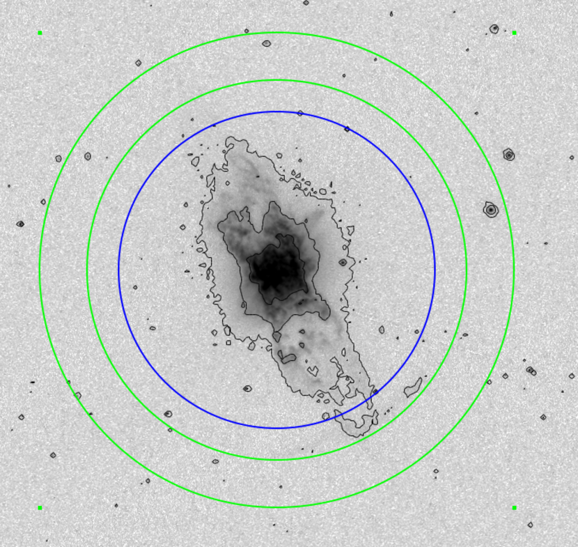
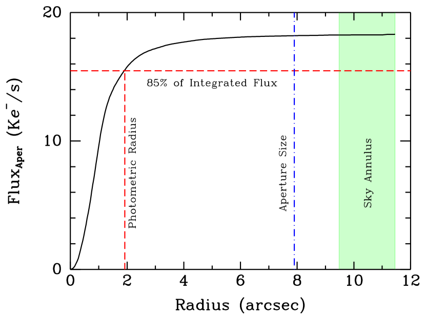
Figure 1: Left: Image of PN G285.4+01.5 with contours (at 10%, 1%, and 0.1% of the maximum target intensity) over plotted. Photometric aperture (blue circle) and sky annulus (green circles) are shown. Right: Curve of integrated flux within the aperture as a function of aperture size, showing the photometric radius (dashed line), the size of the photometric aperture used to determine the flux in F502N (dot-dashed line), and the bounds of the annulus used to determine the sky background (shaded band).

We present all 51 observed targets in the compact Galactic PN image catalog in Appendix A. We determined the dimensions of each nebula by measuring the radius that contains 85% of the integrated light in [O III] $\lambda 5007$, using the Aperture Photometry Tool (Laher et al., 2012) on the F502N images. We measured the flux within a virtual circular aperture with a radius significantly larger than the target, and with brightness clipping to minimize the effect of field stars. The local background was estimated with a circular annulus, again with brightness clipping, using inner and outer radii that were customized for each nebula to be as large as possible. We have used a similar technique systematically in the past (see, e.g., Shaw et al., 2001; Stanghellini et al., 2003; Shaw et al., 2006) with great success. The photometric radius provides a consistent measure of nebular size and is insensitive to the nebular morphology, complexity of the stellar background, and the signal-to-noise ratio in the image. The technique is illustrated in Figure 1 on a highly non-circular PN in our sample, showing the smooth, monotonic rise in the integrated fraction of nebular light with radius.

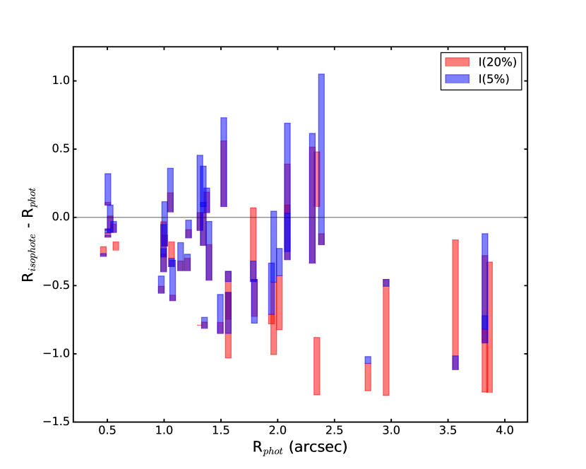
Figure 2: Difference between the nebular radius as determined from our photometric technique (85% of the integrated narrow-band light of [O III] $\lambda 5007$), and that determined from the isophotal contours at 20% (red) and 5% (blue) of the peak intensity in the same band. The bars indicate the range in isophotal radius as determined from the major and minor axis of the nebula.

We also measured the nebular dimensions using one or more isophotes: at 20% of the peak intensity (not counting the CS), at $\sim 5\%$, and in some cases at fainter isophotes if the S/N was high. We measured the diameters along the major and minor axes of the isophote in question, usually on the F502N image unless the S/N was poor, in which case we used the F200LP image. While this technique is the most commonly used (and it can be useful for planning follow-up spectroscopic observations), the results depend strongly upon the S/N ratio in the image and upon the spatial resolution. There is also a level of subjectivity in these measurements, depending for instance on whether microstructure is considered (e.g., ansae), and in choosing how to weight the results for non-circular nebulae. Figure 2 compares our photometric radii with those determined from isophotal contours in the same emission line at two different intensity levels, and for both the major and minor axes. The degree of agreement is very poor and highlights the inconsistency of the isophotal technique, particularly for angularly small nebulae. We note that the statistical distance scale derived by (Stanghellini et al., 2008, hereafter SSV) was calibrated using photometric radii determined in the way described here, and that distances derived using nebular radii as measured in a different waveband or with a different technique are likely to result in significant systematic errors. For these reasons, isophotal radii are certainly not appropriate for deriving physical dimensions of the nebulae, or statistical distances.

We give in successive columns in Table 2 the PN G target designation (column 1), coordinates as measured from the F814W image (columns 2 and 3), the flux in [O III] $\lambda 5007$ and $H\beta$ (columns 4 and 5), the extinction constant at $H\beta$ (column 6), the photometric radius $R_{\rm phot}$ in arcsec, followed by the isophotal diameter(s) and the reference isophote(s) (columns 7, 8, and 9), the morphological class (column 10), and notes on individual nebulae (column 11). Coordinates are given in the ICRS reference system, and correspond to the position of the PN central star if detected, otherwise the approximate geometric center. The [O III] $\lambda 5007$ fluxes are measured directly from the HST images as described above, the $H\beta$ fluxes have been calculated from the [O III] $\lambda 5007/H\beta$ flux ratio from the Acker et al. (1992) catalog. All extinction constants are taken from data published elsewhere, as given in the Table references.

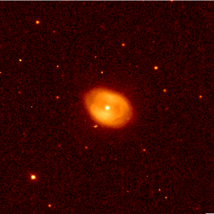
Figure 3: False-color images of PN G264.4–12.7 (left) and PN G327.1–01.8 (right) in the F502N filter, illustrating the R and E morphological types, respectively. Note the faint halo around PN G264.4–12.7. Images are $15\arcsec\times 15\arcsec$, with a log intensity stretch.

We classified the projected morphology of all 51 PNe in the sample based on their appearance in the [O III] $\lambda 5007$ images, following the morphological scheme for Galactic PN morphological classification described in Stanghellini et al. (2006). The major morphological classes are: Round (R) PNe; elliptical (E) PNe, which are distinguished from R PNe if an axial difference of at least $5\%$ is detected; bipolar (B) PNe, implying the presence of at least one pair of lobes, and including quadrupolar and other multi-polar PNe; point-symmetric (P) PNe, implying features with central symmetry and no lobes. We also identified elliptical or round PNe with inner bipolar structure or the presence of a ring as bipolar core (BC) PNe, and set them in a class apart. Some PNe display attached or detached shells or haloes, ansae, and other inner and outer features. These additional, secondary morphological features are noted in column 11. In Figures 3 through 5 we show examples of the principal morphological types. It is worth noting that morphological classification based on imagery alone may be in some cases misleading, since some round or elliptical shapes may derive from bipolar lobes projected into the plane of the sky, and round PNe in particular could also be elliptical in projection. These hidden morphologies can only be detected with the help of nebular kinematic studies (e. g., Kwok 2010), and this is beyond the scope of the present paper, but should be addressed in future studies. Two PNe are not classifiable within the above scheme, and we classify them as Irregular (Irr) in Table 2. The remaining PNe are morphologically distributed into R PNe (2), E PNe (25), BC PNe (4), B PNe (15), and P PNe (3).

3.1 Peculiar Morphologies

While morphological classifications are provided in Table 2 for all observed PNe, several objects have additional features that are worth elaboration. Indeed, macro-morphological details such as the presence of halos indicate that the ionization front has passed completely through the nebula, from which we can infer advanced nebular age and low optical depth to Lyman radiation within the nebula. Other morphological details may suggest shaping by jets, interaction of the nebula with the surrounding ISM, motion of the CS relative to the nebula, and even the presence of toroidal rings which may harbor molecular gas. Even though our classifications are based solely on the projected shape, with no supporting velocity information, these details are clues to the youth or maturity of the nebular evolution.

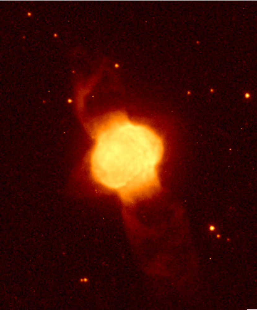
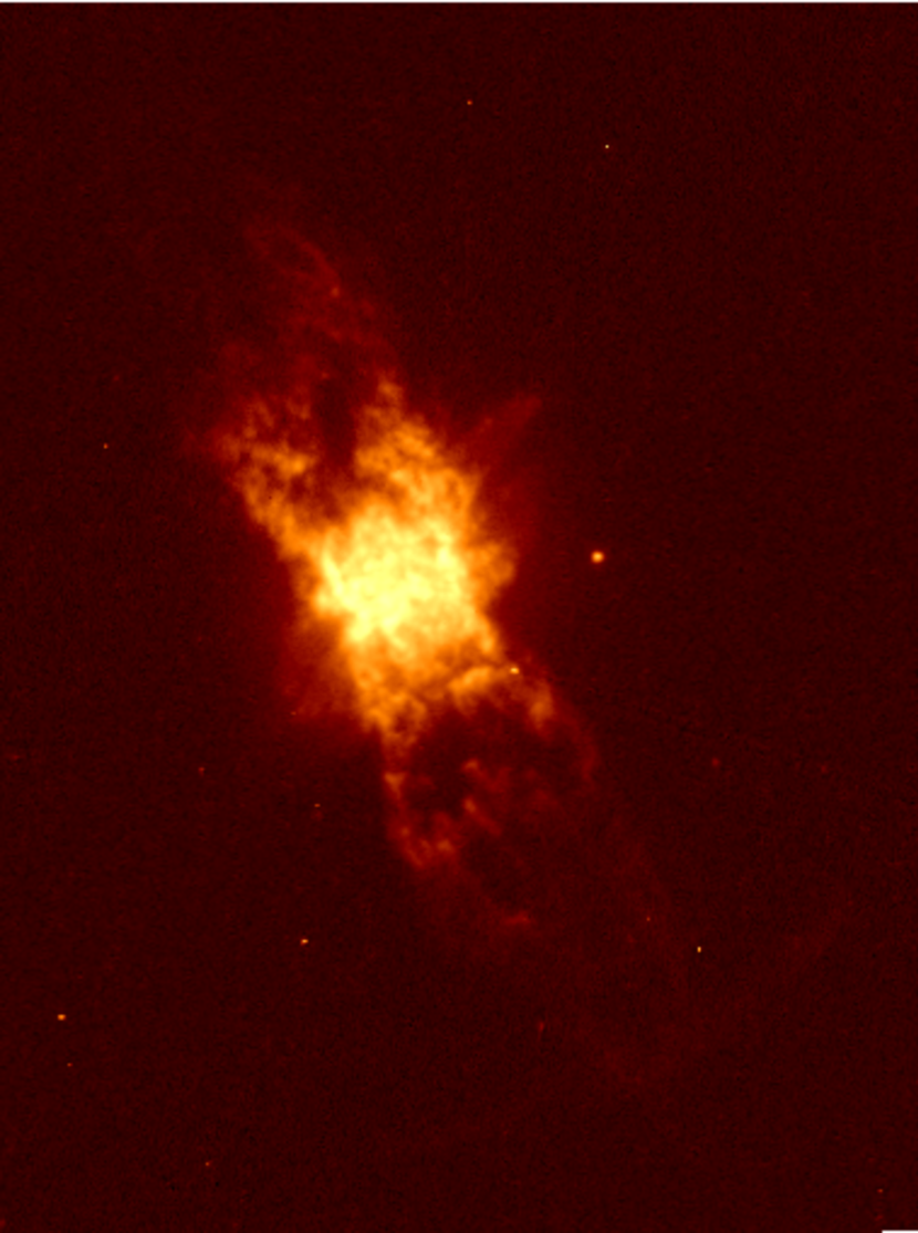
Figure 5: Extended bipolar PNe, PN G021.1-05.9 and PN G285.4+01.5 respectively.

PN G000.8–07.6 (Fig. 5): The bipolar structure of this PN is evident in the [O III] $\lambda 5007$ image. The lobe on the east side of the nebula has been truncated, possibly by interaction with the ISM. Bipolar morphology is preserved close to the CS, i.e., in the region internal to the bow-shock, where the shaping mechanism is not expected to be disrupted (e.g., see Villaver et al. 2012). The bipolar lobe opposite to motion has grown mostly unaltered. The morphology is characteristic of a small relative velocity interaction. Unfortunately there is no proper motion information available for this object for the comparison with dynamical models.

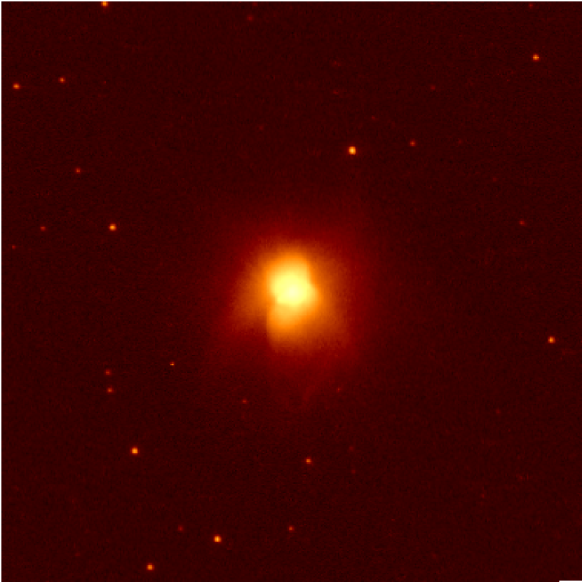
Figure 12: False-color image of PN G000.8–07.6 in the F502N filter.

PN G014.0–05.5 (Fig. 12): The main body of the PN is elliptical, with ansae that could be bipolar lobes seen in projection. The shaping mechanism of this object could be similar to that in the “Cat’s Eye” PN, in at least two phases: Early ejection of a symmetrical shell, and later asymmetrical shaping (Balick et al. 2001, and references therein). Note that PN G026.5–03.0 also shows morphological features indicative of the same two-phase shaping process.

PN G025.3–04.6 (Fig. 14): This PN is multi-polar when looking at the [O III] $\lambda 5007$ image with an appropriate intensity cut.

PN G044.1+05.8 (Fig. 15): This is a very faint PN with an apparently very bright CS. Given the nebular asymmetry and the comparative brightness of the PN and CS, it is possible that the star is not the central remnant, but rather is an unresolved companion or a field star.

PN G053.3+24.0 (Fig. 17): This PN has a bright central ring (probably a torus in projection), with bubble-shaped ansae extending in a direction that could be orthogonal in projection to the plane of the ring. A faint halo extends more than twice the angular size of the ring, with a surface brightness $\sim 1000$ times fainter. Radial structure is evident in the halo, similar to that seen in HST image of NGC 6543 (Balick et al. 2001). The central star is visible in the continuum images, at the center of the ring.

PN G068.7+01.9 (Fig. 18): There is a clear signature of an interaction of this PN with the surrounding ISM, in the form of a rim or a partial ring to the north through west. This feature is easily visible in broad-band continuum, but is quite faint in [O III] $\lambda$5007. It is worth noting that the PN morphology interior to the rim does not appear to be particularly disturbed. The large opening angle of the ring segment could be a bow-shock, which would indicate a low velocity interaction through a low density ISM (Villaver et al., 2012).

PN G107.4–02.6 (Fig. 21): The shape of this PN is highly unusual, if not unique, with an elliptical shell surrounding an oddly shaped main body. Two stars of nearly equal brightness lie within the nebula, separated by 2″: the brighter star is located near the center of the nearly elliptical interior shell, and the fainter star lies near the center of curvature of an extension to the interior shell. Each star appears to lie within a small cavity of lower emission. There is a significant brightness enhancement at the east rim of the interior shell. It is almost as if this PN surrounds two central stars, each of which contributed to the shaping (if not the formation) of the PN, unlikely as that may be given their wide separation. Yet a chance alignment within the nebular shell of a field star of nearly equal brightness to the CS also seems unlikely. This object is worthy of follow-up spectroscopy.

PN G205.8–26.7 (Fig. 22): The shape of this nebula, a round shell surrounding a bright interior ring, with an equatorial brightness enhancement, is characteristic of some early post-AGB stars. Several of the PNe in our survey display this secondary morphology, while none of the non-compact PNe have shown it.

PN G275.3–04.7 (Fig. 24): This PN also has a bright shell surrounding a brighter ring, which is similar to PN G205.8–26.7, except that the equatorial brightness is not as prominent.

PN G285.4+01.5 (Fig. 25): This is a spectacular PN, with remarkable microstructure within the bipolar wings, and on the periphery of the pinched waist. The central star is just visible above the surrounding, bright nebular continuum. There is also a faint arc (invisible with this intensity cut) at the end of one lobe, extending from the west to the northwest, some 8.8″ removed from the CS, which suggests an interaction of the outer shell with the surrounding ISM.

PN G295.3–09.3 (Fig. 27): This PN seems to present extremely early evolution morphology. It is modestly extended in the HST image, and it shows a strong dual ring-like feature. The contours are rectangular in the interior (consistent with a bipolar waist), and the orientation of the rings is consistent with bipolar lobes.

PN G309.5–02.9 (Fig. 29): There is clearly a structure reminiscent of interaction between the PN and the ISM. The opening angle of the putative bow-shock reveals a likely low velocity ( $\approx 20$ Km s^-1) interaction.

PN G327.8–06.1 (Fig. 30): This nebula appears to be multi-polar, with plenty of microstructure. The streak running north-south is probably a diffraction artifact.

PN G344.8+03.4 (Fig. 34): This nebula is very strange. The marginally resolved, bright inner core is shaped like a four-leafed clover, but there is very faint structure in the form of blobs and arcs that are removed from the CS by 5″ to 8″, and lie along one axis of symmetry in the NW and SE. The nebulosity in the outer structure is fainter than the core surface brightness by a factor of 1000. We speculate that a jet may be operative in this very young object.

PN G348.4–04.1 (Fig. 35): The shape of this bright PN looks like a classic pinched waist of a bipolar, except that the lobes seem to be truncated. The CS is quite prominent in the continuum images.

PN G351.3+07.6 (Fig. 36): A bipolar core is distinguishable in this PN, the outer contours of which also square in shape.

PN G356.5+01.5 (Fig. 36): This is a point-symmetric PN with a distinct, asymmetrical arc of emission extending over $180\deg$ on the north side of the nebula. This is a clear signature of interaction with the ISM.

PN G358.6+07.8 (Fig. 37): This elliptical PN shows an inner core and an attached shell, both with a good deal of microstructure that suggests a mature nebula. The CS is very prominent, even in F502N.

3.2 Multiple Ejections, Halos, and Interaction with the ISM

Several PNe show fainter shell structures surrounding the brighter central main nebula. The faint nebula is likely the remnant ejection of mass from the progenitor star as it ascended the asymptotic giant branch (AGB). These structures also represent a clear examples of a shaping mechanism that changes with time, becoming more asymmetrical. PNe showing these features in the sample of compact objects presented here are PN G014.0-05.5, PN G026.5-03.0, PN G052.9-02.7, PN G053.3+24.0, PN G068.7+01.9, PN G079.9+06.4, PN G184.0-02.1, PN G275.3-04.7, PN G309.5-02.9, PN G336.9+08.3, PN G356.5+01.5, and PN G358.6+07.8.

The stellar motion is capable of influencing the structure and dynamics of the ejected AGB envelope, as the stellar mass-loss interacts with the local ISM. As the AGB envelope becomes ionized, marking the birth of the PN, the asymmetries developed from the interaction with the ISM are in many cases major morphological features (Villaver et al. 2012). About $10\%$ of the compact objects under study show morphological features that clearly reveal the interaction between the stellar ejecta and the ISM. This fraction is similar in the compact and the general Galactic PN samples. Note that when deeper images are taken, reveling the external layers, this fraction tends to increase (Corradi et al., 2003).

3.3 Comparison to other classification schemes

Sahai et al (2011, hereafter SMV) studied morphology of pre- and young PNe, and built a morphological classification scheme especially suitable for these early post-AGB ejecta. They analyzed in depth a sample of such targets, determining several physical parameters, and classified them based on their new scheme, including statistical analysis of the resulting distribution among morphological classes.

As a corollary, they shown that their pre- and young-PN morphological scheme is applicable to any given sample of PNe. They used some of the WFC3/HST images publicly available from our snapshot program to prove their point. Their publication occurred when our snapshot survey was still ongoing, and images of only 44 PNe were available (hereafter, the preliminary sample). Their study of the preliminary sample is limited to morphological classification, presented in their Table 5. They did not study the physical parameters, evolution, or distribution amongst morphological classes of the preliminary sample PNe, thus our comparison with their work will be limited to the analysis of the similarities and differences in the classification schemes, and we will also analyze in detail the PNe for which the classification across the two schemes differ.

The morphological class R (round), defined by us for elliptical PNe whose axial difference is $<5\%$, broadly correspond to the R round class in SMV, where round PNe have maximum diameter measuring less than 1.1 times their average diameter. There are two PNe in the preliminary sample that we classify as R, which have been also classified as R by SMV. Our definition is more stringent than that of SMV, thus we expect a few of our elliptical PNe to be classified as round in their scheme.

Our E elliptical PNe class does not have a direct correspondence in SMV’s scheme; nonetheless, they define E elongated PNe as those with elongation along one axis, and we expect most of our E PNe to be classified as elongated by SMV. We indeed found that 13 of the 20 E PNe in the preliminary sample have been classified as E (elongated) by SMV. Three of our E PNe are R in SMV’s scheme; these PNe are those whose ellipticity is below 10 $\%$, and their different classification in the two schemes are compatible within the class definition. The E PN PN G048.5+04.2 is classified as B (bipolar) by SMV. By looking at Figure 16 (left panel) we see why it could not have been defined elongated. We still prefer the E rather than B classification for this target, but we recognize that B is also a possibility. PN G285.4+02.2, which is E in our classification, is irregular in SMV’s. While this target is definitely elliptical, it may not be exactly elongated, thus the respective classifications are agreement within the individual schemes. PN G309.5-02.9 is classified as L by SMV, a class typically used only for pre-PNe; both studies detected the same structures (see Fig. 29, left panel), which we note in $\S$3.1. Finally, the E (or possibly P) PN G344.8+03.4 is classified as S (or, with spiral arms) by SMV, which is compatible with our P class.

Our BC class does not have a correspondence in SMV’s scheme. Following the geometrical definitions of the two schemes, BC PNe should all be classified as E (elongated) by SMV. In fact, all 4 BC PNe in the preliminary sample are classified as E (elongated).

Both our and SMV’s schemes consider B bipolar PNe as a fundamental class. We do not distinguish between bipolar and multipolar PNe, while SMV do (M stands for multipolar in their scheme), but we do include a note to multipolarity in our classification table. There are 12 B PNe in the preliminary sample, and 11 of them are classified as B or M by SMV. In addition, the B PN PN G042.9-06.9 (Fig. 15, left panel) is L in SMV classification, which is compatible with B in our scheme.

We use the separate class P to indicate point-symmetry, while a similar main class is not included in SMV’s scheme. Of the 3 P PNe of the preliminary sample, two (PN G025.3-04.6 , Fig. 14, left panel; and PN G356.5+01.4, Fig. 36, right panel) are classified as elongated, which is how we would have classified if we were working with SMV’s scheme. The third one, PN G296.3-03.0 (Fig. 28, left panel) is classified as B by SMV. While the PN has a pinched waist, we do not see the axial-symmetry that is expected in a bipolar PN, while we do see the point-symmetry. This may be the target where the respective classifications definitely diverge.

We classify 2 PNe in the preliminary sample as irregular: PN G309.0+00.8 (Fig. 28, right panel) and PN G98.2+04.9 (Fig. 20, right panel), respectively bipolar and elongated in SMV’s paper. The former PN may be bipolar (or multipolar) with evolved morphological pattern, although we prefer to classify it as irregular. The latter PN is definitely elongated, but not elliptical, thus both classifications agree within the respective schemes.

To summarize this comparison, there are three PNe (PN G48.5+04.2, PN G309.0+00.8, and PN G296.3-03.0) whose morphology we believe may be different from SMV’s classification, once taken into account the different schemes. Misclassification represent a very small fraction of the preliminary sample, thus a comparable analysis as we present in this paper but using SMV’s morphological scheme would have very similar outcome.

3.4 Distances and Physical Sizes

We did not know a priori whether to attribute the small sizes of the target PNe to young dynamical age or large distance. PNe would be dynamically younger than 2000 yr if they are angularly smaller than $\sim 4\arcsec$ and closer than 6 kpc (Villaver et al., 2002). Only by measuring statistical distances could we establish whether a compact PN is young or merely distant. But statistical distances are based on apparent radii, which has been impossible for compact PNe before the HST images became available. It is worth noting that apparent PN radii smaller than 4″ are always extremely uncertain if measured from ground-based images, thus not sufficient to soundly determine whether the nebula is dynamically young or just located at larger distance.

Once we measured the photometric radii, the distances to the PNe were determined via the standard statistical techniques, as described by SSV. In order to determine the distances we follow Eqs. 8ab of SSV, which give the distances to the PNe if the angular radius, the 5 GHz flux, and the optical thickness parameter $\tau$ are available. For our calculation, we used the measured photometric radii ($R_{\rm phot}$) listed in Table 2. We used the 5 GHz fluxes from Cahn et al. (1992, hereafter CKS). In the cases where the 5 GHz flux was not available in CKS, we utilized the $F_{\rm\nu}$(5 GHz) to $F_{\rm H\beta}$ relation (see CKS, Eq. 6), using for input the $H\beta$ flux and extinction constant from Table 2.

The resulting distances, and physical sizes, of the PNe are given in Table 3, where we give the $F_{\rm\nu}$(5 GHz), the flux adopted for the distance calculation in column (2), its reference in column (3), which also indicated the cases where the 5 GHz flux had been inferred from the $H\beta$ flux. Column (4) gives the calculated optical thickness parameter $\tau$, which determines the formula used to calculate the distance (see SSV). Columns (5) through (8) give the physical parameters dependent on the distance scale, respectively, the physical radius $R$, the PN distance from Earth $D$, the PN distance from the Galactic center $R_{\rm G}$, and the absolute scale-height from the Galactic plane, $|z|$. For PNe whose morphology is markedly bipolar we use the distance scale based on the relation between surface brightness and size, as explained in SSV.

In addition to those deselected at proposal time, few additional compact PNe may be members of the Galactic halo or bulge population, based on our new distances, and following the prescription by SH10. The possible halo PNe in our sample are PNG 53.3+24.0, PN G264.4-12.7, and PN G275.3-04.7; possible bulge PNe are PN G000.8-07.6, PN G356.5+01.5, and PN 358.6+07.8.

4 The Correlation of Nebular Morphology and Dust Type

Most (45) of our targets have simultaneous HST images and Spitzer/IRS observations, thus we can relate the dust type to other characteristics for the Galactic PN sample. We use the dust type classes as described by Stanghellini et al. (2012). These classes are based on the $4-40~{}\mu$m spectra of the PNe, displaying either carbon dust features, which may include either or both aromatic and aliphatic dust emission (carbon-rich dust, or CRD); oxygen-dust features, which may include either or both crystalline and silicates (oxygen-rich dust types, or ORD); or both dust types (mixed-chemistry dust, or MCD). In some cases, there are no visible features above the dust continuum (featureless, or F). If we separate the PNe into two morphological groups, namely, “spherical” (R and E: 26 PNe) and “aspherical” (B, BC, and P: 19 PNe), we can see evident differences in the dust type distributions of the two groups. In fact, most ($\sim 60\%$) spherical PNe are CRD, while only $\sim 17\%$ of them are ORD. The situation is reversed for aspherical PNe, where a large fraction of PNe ($\sim 47\%$) are ORD, and only $25\%$ are CRD. MCD PNe are respectively $8$ and $16\%$ of the spherical and aspherical samples. Featureless PNe are frequent in the spherical ($25\%$) sample, but not among the aspherical ones ($5\%$). Stanghellini et al. (2007, 2012) have shown that lack of molecular features above the continuum in IRS spectra are linked to more evolved PNe, both in the Galactic than in the Magellanic Cloud samples. It seems clear that overall the aspherical sample has more un-evolved targets, both in the compact and general Galactic samples.

5 Compact Galactic PNe Compared to the General Galactic Population

In order to acquire a deeper knowledge of our ensemble of compact Galactic PNe (hereafter, the “compact sample”) one should study them in the context of the general Galactic population. We use the general sample of spectroscopically-confirmed PNe from the Acker et al. (1992) catalog. Physical parameters for all but the compact sample are taken directly from SH10, where all Galactic PNe in the Acker et al. (1992) catalog had been searched for reliable published physical parameters. In other words, the database used here is the same as in SH10, with the exception of morphologies, physical sizes, and distances of compact sample, which are from this paper.

There are 938 Galactic PNe whose radii and statistical distances are known to date. The compact sample consists of all 51 PNe listed in Table 3. In all the following comparisons we include the compact sample in the general Galactic sample, unless otherwise noted. Also, the general and the compact samples have been scaled by number for easy comparison in the plots.

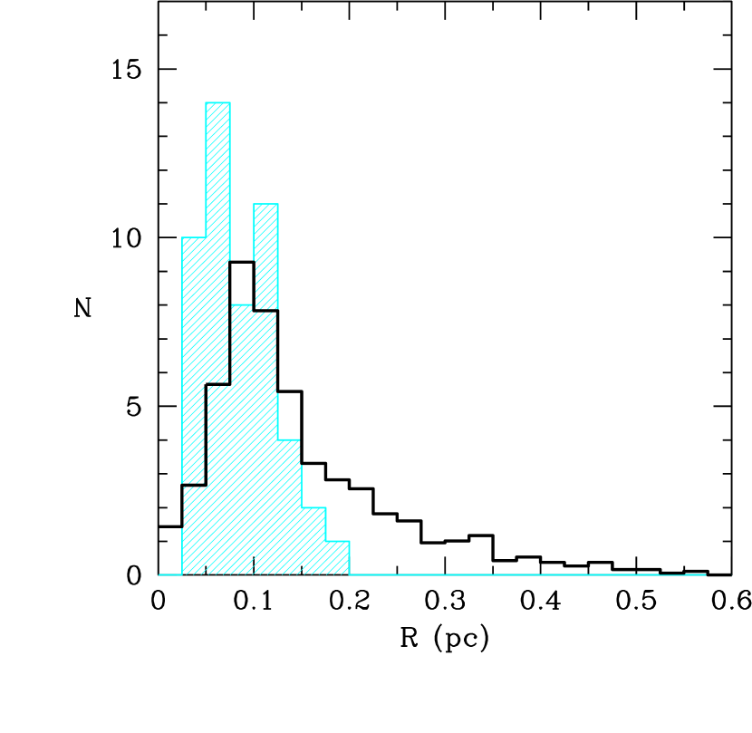
Figure 6: Histogram of the physical, radial size of compact Galactic PNe (shaded, cyan) compared to that of all Galactic PNe (black). The total number of PNe have been scaled for easier comparison. Physical radii have been determined from photometric radii and statistical distances.

In Figure 6 we show the distribution of physical sizes of the compact sample (shaded histogram) compared to the general sample (thick histogram). It is evident from this figure that selecting apparently compact PNe excludes the most extended nebulae, i.e., those with radii larger than $\sim 0.2$ pc when calculated based on the SSV distance scale. But in order to determine what fraction of compact PNe are dynamically young we need to examine their optical thickness, and distance, distributions.

In order to discriminate between optically-thin and optically-thick PNe, we use the optical thickness parameter $\tau$, given for the compact sample in Table 3. Optically-thick (or radiation-bounded) PNe have $\tau<2.1$, and their ionized mass depends on the progression of the ionization front toward the outer edge of the nebula. Optically-thin (or density-bounded) PNe have $\tau>2.1$, their nebular ionized mass is assumed constant in this approximation, and the nebular gas is completely ionized within the nebula. This is based on a very simple PN model, yet it can be used as an additional tool to determine the evolutionary stage of compact Galactic PNe. We found that $<\tau>=3.65\pm 1.21$ for the general sample. On the other hand, $<\tau>=2.7\pm 0.85$ when calculated for the compact sample exclusively, indicating that a larger fraction of PNe in the compact sample are optically-thick, compared to the general sample. Yet the majority of the compact sample PNe are optically thin, as is the majority of the general sample. In summary, dynamically young, optically-thick PNe are more abundant amongst the compact sample than the general sample; nonetheless, they do not represent the majority of the former sample, and most of the compact sample PNe are evolved and optically-thin.

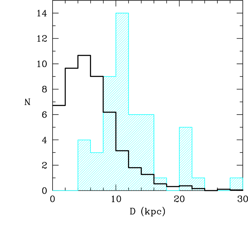
Figure 7: Distance distribution of compact Galactic PNe (shaded, cyan) compared to that of all Galactic PNe (black). The total number of PNe have been scaled for easier comparison.

In Figure 7 we show the distance distribution of compact sample PNe (shaded histogram), compared to that of the general sample. All distances have been determined with the statistical scheme by SSV. By selecting angularly compact PNe, as done to build the compact sample, we probe distances that cluster around 10–12 kpc, and also probe the farther reaches of the Galaxy, while the general sample PNe resides within $\sim 10$ kpc, and peaks around 5 kpc. Only a few PNe in the compact sample are closer than 6 kpc, thus dynamically young.

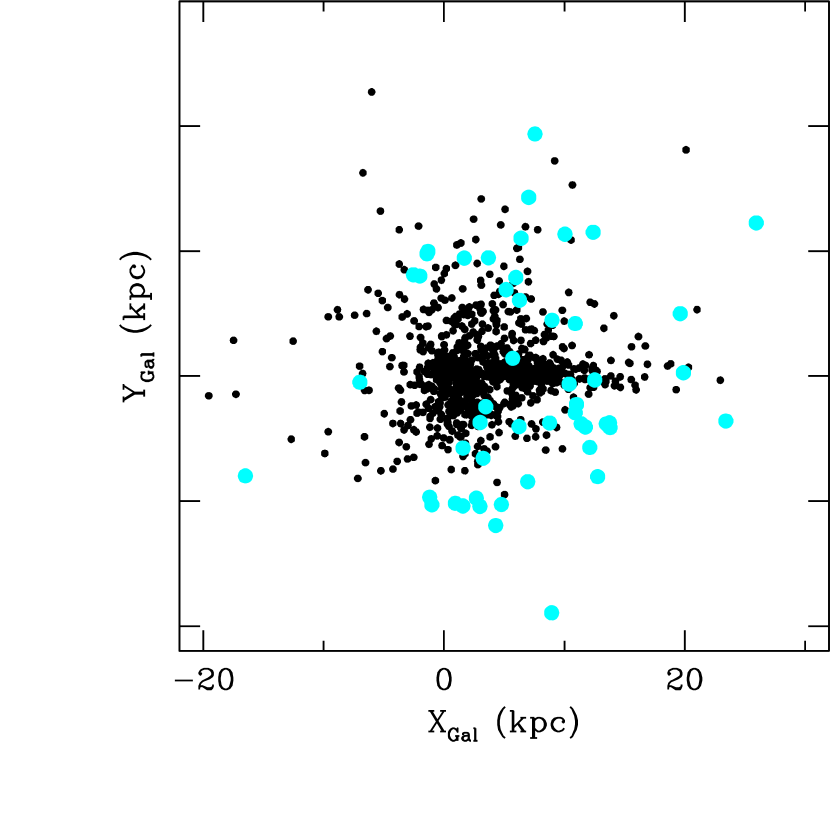
Figure 8: Spatial distribution of compact Galactic PNe (large, cyan dots) against the general distribution of Galactic PNe (small, black dots).

In Figure 8 we show the Galactic distribution of the compact sample (large dots) with respect to the general Galactic sample (black dots). Here we plot the $X_{\rm Gal}=Dcos(b)cos(l)$ and $Y_{\rm Gal}=Dcos(b)sin(l)$, where $l$ and $b$ and the target’s longitude and latitude. It is important to note that the compact sample PNe generally populate the Galaxy periphery, rather than its center. Generally speaking, PNe in the compact sample are seen at farther distances than the general sample, as also seen in Figure 7. It is worth recalling that HST observations did not privileged any particular sector of the Galaxy when observing a subsample of the original target list, thus selection effects are unlikely. All Galactic PN with known distances, including bulge and halo PNe, have been included in Figure 8; disallowing possible bulge and halo PNe would not change the plot significantly.

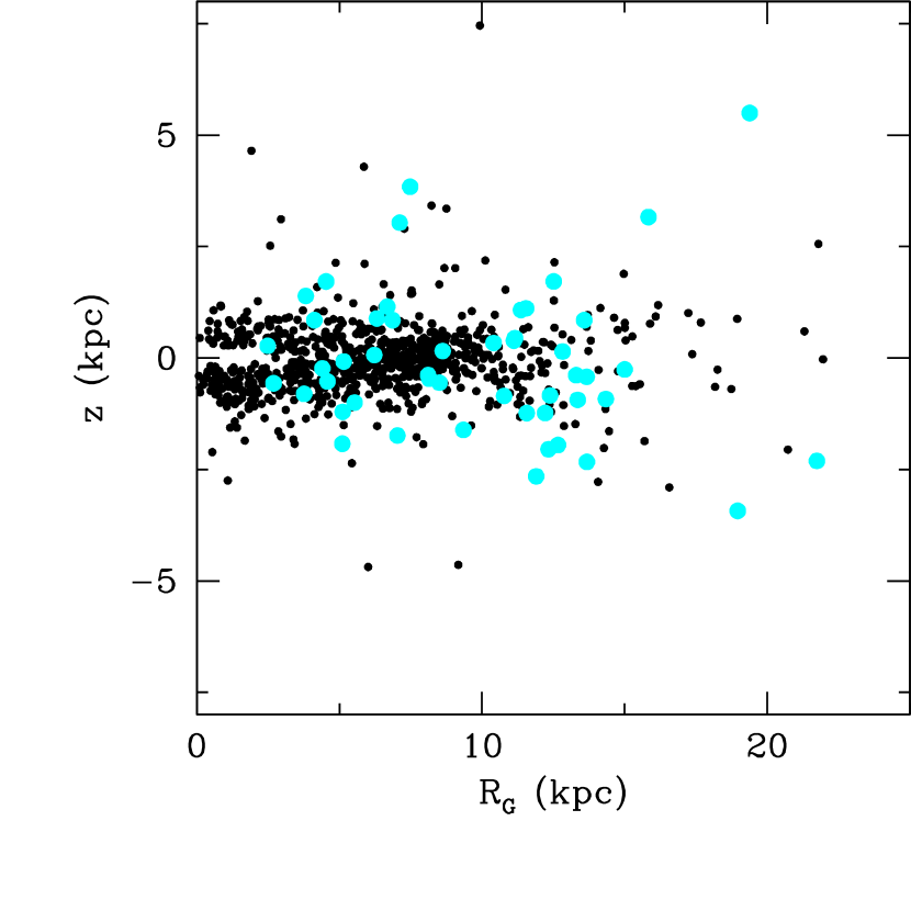
Figure 9: Spatial Radial distribution vs. distance from the galactic plane, z of compact Galactic PNe (large, cyan dots) against the general distribution of Galactic PNe (small, black dots).

More insight can be obtained by looking at the distribution of the compact sample in the $z-R_{\rm G}$ plane, as in Figure 9, where $z$ is the distance form the Galactic plane, and $R_{\rm G}$ is the radial distance from the Galactic center, calculated as in SH10. We found that the compact sample PNe (large dots) are not concentrating in any particular location of the Galaxy with respect to the general sample, showing that they represent the general PN population both in scale height and galactocentric radius. The plot shows that the compact sample is not tightly confined to the proximity of the Galactic plane. In fact, the average absolute distance of the compact sample PNe from the plane is $<|z|>=1.42\pm 1.57$ kpc, compared to $<|z|>0.66\pm 1.22$ kpc of the general sample. This finding agrees with the population of the compact sample being just a subsample of the general population, i.e., these compact PNe are merely, on average, farther away from us than the general population. Distances from the Galactic center of compact PNe cover the same domain than the general population, as seen in Figure 9, although the average galactocentric distance of compact PNe is $<R_{\rm G}>=10.10\pm 5.01$ kpc, against the complete sample with average $6.56\pm 4.14$ kpc, showing that compact sample PNe probe the farther reaches of the Galaxy.

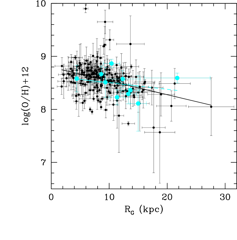
Figure 10: Radial oxygen gradient for Galactic PNe, excluding the bulge and halo population. The general PN population (filled, black dots) are contrasted with the compact PNe (large cyan dots). Gradients have been fit to the complete (solid line) and compact (broken line) populations.

In Figure 10 we show the radial oxygen abundance distribution of compact sample (large dots) and that of the general sample. Here we excluded bulge and halo PNe. Oxygen abundances are from SH10, except that the SH10 database has been updated with the abundances by García-Hernández & Górny (2014), from which we chose only those PNe observed directly by the Authors, and by Dufour et al. (2015). By plotting metallicity vs. galactocentric radius, we have a sample of 206 disk PNe whose oxygen abundance is known from direct abundance analysis. The radial oxygen gradient of all these PNe is shallow, with slope of $\Delta{\rm log}(O/H)/\Delta R_{\rm G}=-0.026$ dex kpc^-1, and intercept ${\rm log}(O/H)+12=8.8$. By selecting only compact sample PNe we obtain a metallicity gradient gradient slope of $\Delta{\rm log}(O/H)/\Delta R_{\rm G}=-0.013$ (dex kpc^-1) and intercept ${\rm log}(O/H)+12=8.63$. The difference in gradient slopes is not significant, given the large scatter of the distributions. The average oxygen abundance of the general sample is slightly higher than that of the compact sample, but the number of PNe in the compact sample with known oxygen abundance is still too small to draw evolutionary conclusions based on these averages. The fact that compact PNe probe farther Galactic regions implies that this sample has more potential for improving the estimates of the O/H gradient in the Galaxy, and should be followed up with more spectroscopic analysis in the future.

There are other ways to assess the distribution of our compact sample within the Galaxy. For example, by comparing the optical extinction distribution of Galactic PNe for which extinction at $H\beta$ is reliable (see SH10), we obtain an average $c_{\beta}=1.25\pm 0.87$, which is very similar to what obtained for the compact sample, $c_{\beta}=1.12\pm 0.72$. This indicates that PNe of the compact sample do not reside at particularly high extinction patch of the Galaxy.

We have compared the frequency of morphological distribution of the compact sample to those of the general sample. We could assign 579 Galactic PNe to a definite morphological class, including the compact PNe with known morphology studied in this paper. About half of both the general ($48\%$) and the compact ($51\%$) sample are elliptical . The other half is divided between R (approximately $14$ and $4\%$ of the general and compact samples respectively), BC ($\sim 15$ and $8\%$), B ($\sim 19$ and $31\%$), and P ($\sim 6$ and $3\%$). If we group B and BC PNe into one class, then the percentages of these PNe are very similar for the general ($35\%$) and the compact ($39\%$) samples, which may indicate that the different BC and B fraction of the two groups may be due to higher definition of the HST images. In fact, most of the morphological class assignment of the extended PNe is based on ground-based images. Similarly, the higher fraction of R and P PNe in the general group may also be due to an image definition issue. We are inclined to believe that the morphological distribution of the compact sample is very similar to that of the general sample. This strengthens the conclusion that the compact sample is representative of the general PN population in the Galaxy.

6 Discussion

The main goal of this project was to present a morphological catalog of compact, Galactic PNe, through narrow-band images (Appendix A), and to explore the detailed properties of this understudied class of PN. The observed targets were selected based on their compact size. The 130 original targets represent a large fraction of all spectroscopically-confirmed Galactic PNe whose ground-based measured radius is smaller than 4″. The further selection down to the 51 PNe presented here is due mostly to random sky position available for the snapshot program to be activated, thus is similarly distributed to the original selection, although it could slightly favor brighter PNe, which are observable in shorter time slots. Our compact sample is representative of all compact PNe in the Galaxy.

We did not know a priori that this sample would result in a representative Galactic PN sample, which is slightly skewed to more distant PNe, and with a higher-than-average optically-thick, radiation-bounded PN fraction. One of the original goals of this survey was to study the early onset of morphology, assuming that the majority of compact PNe would be also young, i.e., recently ejected, and with a short dynamical age. This does not appear to be the case after studying the sample against a homogeneous Galactic sample of both compact and extended PNe. Most of the compact sample PNe are not in an earlier dynamical evolutionary stage than the general Galactic PN population, although the fraction of optically-thick PNe is higher in the compact sample ($\sim 40\%$) than in the general sample ($\sim 11\%$ ).

We perform morphological classification of the nebulae based on projected shapes. The morphological distribution of PNe in the Galaxy is not very different if the PNe are compact or extended, as it appears, if we consider the broad morphological groups of spherical (R and E) and aspherical (B, BC, and P) PNe. On the other hand, there are notably more lobed B PNe among the compact than the general sample, with BC/B number ratio being $90\%$ in the general group and only $30\%$ in the compact sample. An important distinction between the compact and general samples is that morphology of compact PNe are all from HST images, thus the definition of certain details may be superior to those of ground-based images which constitute the majority of all PN images available to date for Galactic PNe. This could augment the relative number of B PNe relative to the BC PNe that one would observe from the ground at a lesser resolution. A direct comparison of our morphological classification with that of SMV’s shows differences in only 3 targets, making both classification schemes reliable and non subjective.

To reinforce the conclusion that compact sample belongs to a general population is their extinction and spatial distributions. They are distributed through the Galaxy, with relative predominance toward the larger galactocentric radii, making them ideal probes to determine Galactic metallicity gradients. Compact sample PNe may be on average brighter than the general population. It is beyond the scope of this paper to perform a detailed study of the luminosities of the two populations, but we can calculate the [O III] $\lambda 5007$ equivalent magnitudes for all PNe discussed here that have a flux determination, and determine their absolute magnitude distribution based on the statistical distances.

In Figure 11 we show the absolute equivalent magnitude distribution in the light of [O III] $\lambda 5007$ for the compact sample (shaded histogram) and the general sample (thick histogram). The [O III] $\lambda 5007$ equivalent absolute magnitude has been calculated from the standard formulation: $M_{\rm 5007}=-2.5{\rm log}(I_{\rm 5007})-13.74$, where $I_{\rm 5007}$ is the absolute intensity in the line at 10 pc. There are 778 PNe, 45 of which compact, whose absolute [O III] $\lambda 5007$ magnitude is known, and that have been included in Fig. 11. The compact PN distribution peaks at lower absolute magnitudes than the general sample, and their distribution also lacks the lower luminosity tail that is seen in the general sample. This strengthen the finding that compact Galactic PNe, while similar in population than the general Galactic PN sample, are a brighter subset of the general Galactic sample, and can be found at larger distances.

7 Conclusions and Future Work

We have present the catalog of compact Galactic PNe, based on HST/WFC3 images. We have determined photometric radii, distances, morphological types, and other physical characteristics of this nebular sample, which has been homogeneously and unbiasedly selected form the general Galactic PN sample, based on apparent sized being smaller than 4″.

The compact sample presented here has unique attributes, in the simultaneous availability of their HST images—thus photometric and morphological properties presented here, and the central stars studies presented elsewhere—and Spitzer IRS spectra, ideally suited to disclose their dust and molecular properties. Once high quality optical spectra become available the abundances will be highly accurate because the collisionally excited IR lines in our IRS spectra offer more diagnostics and ionic species not seen in the optical. An optical spectroscopic program is already underway.

Morphological analysis of the PNe distributes them into the commonly used macro- morphological classes, with similar spherical to non-spherical number ratios than the general population, except the compact sample includes more bipolar members than the general sample.

We determined physical radii and distances of the observed PNe, examined their distribution within the Galaxy, and compared it with that of the general Galactic sample. We found that not all PNe in the compact sample are dynamically young, and the majority of them represents a typical Galactic PN population, with their distribution skewed toward more distant, and brighter, PNe, allowing to peer into the far reaches of the Galaxy. The studied sample is typical of the larger, general population except that it excludes physically large PNe, and has a higher proportion of quite small PNe.

It is worth noting that another sample of compact Galactic PNe would not necessarily have the same properties of the one presented here: let us recall that we did not add any selection bias a priori, and that we confirmed a posteriori that the sample is representative of the Galactic PN population.

Our conclusions have a broader impact. In particular, in the next decade or so astronomers will finally be able to determine absolute physical properties of Galactic PNe based on GAIA distances, which are expected to be much more accurate than the statistical distances. We will be able to use directly the GAIA distances and all the related physical properties presented here and elsewhere of this particular Galactic PN sample as the most complete to date.

Appendix A The Catalog of compact Galactic PNe

In this Appendix we show the images of all compact Galactic PNe observed. Figure Set 12 shows the compact Galactic PN images through the F502N filter, from our program, except for PN G348.8-09.0, where we show the F200LP image (its F502N image is not available). Typically, images are $15\arcsec\times 15\arcsec$, with the exception of the few very large PNe, with a log intensity stretch. The complete catalog with images in all filters will be published in the near future in a dedicated webpage within the MAST HLSP archive.

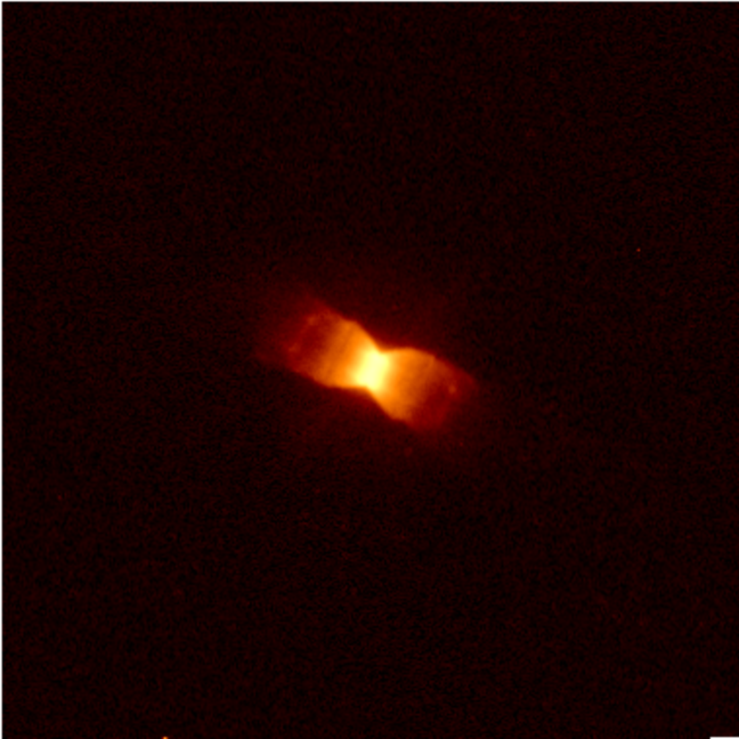
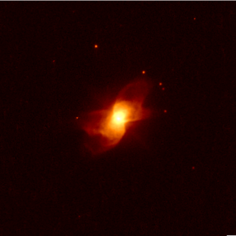
Figure 4: Same as Figure 3 for PN G286.0–06.5 (left) and PN G327.8–06.1 (right), illustrating the B and multi-polar morphological types, respectively.

Figure 11: The distribution of absolute equivalent magnitudes for Galactic PNe with known [O III] $\lambda 5007$ flux and distance. Compact Galactic PNe are represented by the shaded histogram, while the general Galactic sample is in black. The two histograms have been scaled for direct comparison.

Fig. Set12. All Compact Galactic PNe observed

Table 1: Observing Log

PN G	Name	UT Date	Dataset	Filter	texp	PA
					(s)	(deg)
(1)	(2)	(3)	(4)	(5)	(6)	(7)
000.8–07.6	H2–46	2010 Mar 07	IB1B05011	F502N	375, 375	130.1
			IB1B05020	F200LP	20, 2
			IB1B05030	F350LP	20, 2
			IB1B05UNQ	F814W	25
011.7–06.6	M1–55	2009 Sep 04	IB1B23011	F502N	50, 50	-48.3
			IB1B23020	F200LP	30, 3
			IB1B23030	F350LP	30, 3
			IB1B23RIQ	F814W	32
014.0–05.5	VV3–5	2009 Sep 22	IB1B27011	F502N	50, 50	-48.3
			IB1B27020	F200LP	60, 6
			IB1B27030	F350LP	60, 6
			IB1B27PJQ	F814W	40
014.3–05.5	VV3–6	2009 Sep 17	IB1B28011	F502N	50, 50	-47.9
			IB1B28020	F200LP	50, 5
			IB1B28030	F350LP	50, 5
			IB1B28WQQ	F814W	38
021.1–05.9	M1–63	2009 Oct 11	IB1B34011	F502N	300, 300	-51.4
			IB1B34020	F200LP	20, 2
			IB1B34030	F350LP	20, 2
			IB1B34F7Q	F814W	27
025.3–04.6	K4–8	2010 Mar 5	IB1B38011	F502N	30, 30	137.0
			IB1B38020	F200LP	20, 2
			IB1B38030	F350LP	20, 2
			IB1B38DJQ	F814W	30
026.5–03.0	Pe1–19	2010 Feb 22	IB1B40011	F502N	300, 300	142.3
			IB1B40020	F200LP	40, 4
			IB1B40030	F350LP	40, 4
			IB1B40CLQ	F814W	35
042.9–06.9	NGC 6807	2009 Aug 07	IB1B48011	F502N	100, 100	-1.4
			IB1B48020	F200LP	20, 2
			IB1B48030	F350LP	20, 2
			IB1B48PYQ	F814W	25
044.1+05.8	CTSS–2	2010 Aug 30	IB1B49011	F502N	300, 300	-26.5
			IB1B49020	F200LP	80, 8
			IB1B49030	F350LP	80, 8
			IB1B49ARQ	F814W	46
048.5+04.2	K4–16	2010 Mar 01	IB1B52011	F502N	100, 100	153.2
			IB1B52020	F200LP	120, 12
			IB1B52030	F350LP	120, 12
			IB1B52I7Q	F814W	52
052.9–02.7	K3–41	2009 Oct 03	IB1B56011	F502N	300, 300	-45.2
			IB1B56020	F200LP	60, 6
			IB1B56030	F350LP	60, 6
			IB1B56SXQ	F814W	40
053.3+24.0	Vy1–2	2010 Feb 02	IB1B57011	F502N	300, 300	168.0
			IB1B57020	F200LP	10, 1
			IB1B57030	F350LP	10, 1
			IB1B57A7Q	F814W	23
059.9+02.0	K3–39	2009 Dec 29	IB1B61011	F502N	300, 300	-116.6
			IB1B61020	F200LP	120, 75
			IB1B61030	F350LP	120, 75
			IB1B61LEQ	F814W	120
063.8–03.3	K3–54	2009 Nov 02	IB1B63011	F502N	150, 150	-61.6
			IB1B63020	F200LP	20, 2
			IB1B63030	F350LP	20, 2
			IB1B63DSQ	F814W	30
068.7+01.9	K4–41	2010 Jan 30	IB1B64011	F502N	100, 100	-152.2
			IB1B64020	F200LP	110, 11
			IB1B64030	F350LP	110, 11
			IB1B64CMQ	F814W	50
068.7+14.8	Sp4–1	2009 Jul 30	IB1B65011	F502N	30, 30	17.4
			IB1B65020	F200LP	20, 2
			IB1B65030	F350LP	20, 2
			IB1B65CPQ	F814W	25
079.9+06.4	K3–56	2009 Oct 02	IB1B67011	F502N	690, 690	-31.6
			IB1B67020	F200LP	80, 8
			IB1B67030	F350LP	80, 8
			IB1B67LTQ	F814W	46
097.6–02.4	M2–50	2009 Nov 15	IB1B69011	F502N	300, 300	-50.8
			IB1B69020	F200LP	50, 5
			IB1B69030	F350LP	50, 5
			IB1B69VFQ	F814W	36
098.2+04.9	K3–60	2009 Dec 04	IB1B70011	F502N	300, 300	-72.9
			IB1B70020	F200LP	120, 80
			IB1B70030	F350LP	120, 80
			IB1B70WXQ	F814W	38
104.1+01.0	Bl2–1	2009 Oct 12	IB1B71011	F502N	150, 150	-6.3
			IB1B71020	F200LP	120, 75
			IB1B71030	F350LP	120, 75
			IB1B71FNQ	F814W	110
107.4–02.6	K3–87	2009 Nov 29	IB1B0M011	F502N	710, 710	-51.2
			IB1B0M020	F200LP	60, 6
			IB1B0M030	F350LP	60, 6
			IB1B0MLUQ	F814W	42
184.0–02.1	M1–5	2009 Sep 03	IB1B73011	F502N	150, 150	133.7
			IB1B73020	F200LP	20, 2
			IB1B73030	F350LP	20, 2
			IB1B73JHQ	F814W	30
205.8–26.7	MaC2–1	2009 Nov 11	IB1B74011	F502N	30, 30	-170.9
			IB1B74020	F200LP	10, 1
			IB1B74030	F350LP	10, 1
			IB1B74OXQ	F814W	20
263.0–05.5	PB 2	2010 Jan 02	IB1B75011	F502N	300, 300	-157.1
			IB1B75020	F200LP	30, 3
			IB1B75030	F350LP	30, 3
			IB1B75H5Q	F814W	33
264.4–12.7	He2–5	2009 Oct 04	IB1B76011	F502N	150, 150	124.9
			IB1B76020	F200LP	20, 2
			IB1B76030	F350LP	20, 2
			IB1B76ZCQ	F814W	24
274.1+02.5	He2–34	2009 Dec 08	IB1B77011	F502N	300, 300	164.1
			IB1B77020	F200LP	120, 54
			IB1B77030	F350LP	120, 54
			IB1B77HLQ	F814W	100
275.3–04.7	He2–21	2009 Oct 17	IB1B78011	F502N	300, 300	118.2
			IB1B78020	F200LP	120, 3
			IB1B78030	F350LP	120, 3
			IB1B78KCQ	F814W	32
278.6–06.7	He2–26	2009 Oct 24	IB1B79011	F502N	15, 15	123.1
			IB1B79020	F200LP	20, 2
			IB1B79030	F350LP	20, 2
			IB1B79BFQ	F814W	27
285.4+01.5	Pe1–1	2009 Oct 05	IB1B80011	F502N	300, 300	82.9
			IB1B80020	F200LP	120, 16
			IB1B80030	F350LP	120, 16
			IB1B80GIQ	F814W	60
285.4+02.2	Pe2–7	2009 Aug 17	IB1B81011	F502N	50, 50	30.7
			IB1B81020	F200LP	70, 7
			IB1B81030	F350LP	70, 7
			IB1B81C8Q	F814W	42
286.0-06.5	He2–41	2009 Oct 20	IB1B82011	F502N	30, 30	104.9
			IB1B82020	F200LP	30, 3
			IB1B82030	F350LP	30, 3
			IB1B82T5Q	F814W	30
289.8+07.7	He2–63	2009 Dec 05	IB1B83011	F502N	300, 300	141.6
			IB1B83020	F200LP	20, 2
			IB1B83030	F350LP	20, 2
			IB1B83B9Q	F814W	24
294.9–04.3	He2–68	2009 Nov 03	IB1B84011	F502N	50, 50	97.7
			IB1B84020	F200LP	100, 10
			IB1B84030	F350LP	100, 10
			IB1B84G0Q	F814W	50
295.3–09.3	He2–62	2009 Oct 29	IB1B85011	F502N	30, 30	93.9
			IB1B85020	F200LP	20, 2
			IB1B85030	F350LP	20, 2
			IB1B85RYQ	F814W	26
296.3–03.0	He2–73	2009 Dec 06	IB1B86011	F502N	300, 300	132.2
			IB1B86020	F200LP	80, 8
			IB1B86030	F350LP	80, 8
			IB1B86RGQ	F814W	45
309.0+00.8	He2–96	2010 Jan 22	IB1B87011	F502N	300, 300	147.7
			IB1B87020	F200LP	120, 20
			IB1B87030	F350LP	120, 20
			IB1B87AUQ	F814W	64
309.5–02.9	MaC1–2	2010 Mar 13	IB1B88011	F502N	100, 100	-173.0
			IB1B88020	F200LP	120, 20
			IB1B88030	F350LP	120, 20
			IB1B88ZTQ	F814W	66
311.1+03.4	He2–101	2010 Jan 20	IB1B89011	F502N	300, 300	148.7
			IB1B89020	F200LP	120, 15
			IB1B89030	F350LP	120, 15
			IB1B89QJQ	F814W	60
324.8–01.1	He2–133	2010 Mar 15	IB1B91011	F502N	500, 500	160.8
			IB1B91021	F200LP	120, 120
			IB1B91031	F350LP	120, 120
			IB1B91AOQ	F814W	120
327.1–01.8	He2–140	2009 Aug 28	IB1B93011	F502N	630, 630	-33.8
			IB1B93020	F200LP	120, 20
			IB1B93030	F350LP	120, 20
			IB1B93FHQ	F814W	60
327.8–06.1	He2–156	2010 Aug 21	IB1B94011	F502N	300, 300	-43.3
			IB1B94020	F200LP	20, 2
			IB1B94030	F350LP	20, 2
			IB1B94FHQ	F814W	30
334.8–07.4	He3–1312	2009 Jul 28	IB1B97011	F502N	30, 30	-66.1
			IB1B97020	F200LP	20, 2
			IB1B97030	F350LP	20, 2
			IB1B97HNQ	F814W	30
336.9+08.3	He3–1312	2010 May 11	IB1B98011	F502N	50, 50	-162.8
			IB1B98020	F200LP	90, 9
			IB1B98030	F350LP	90, 9
			IB1B98HNQ	F814W	50
340.9–04.6	Sa1–3	2010 Jan 20	IB1B99011	F502N	100, 100	121.2
			IB1B99020	F200LP	100, 10
			IB1B99030	F350LP	100, 10
			IB1B99HJQ	F814W	50
341.5–09.1	He2-248	2010 Aug 06	IB1B0A011	F502N	30, 30	-54.0
			IB1B0A020	F200LP	20, 2
			IB1B0A030	F350LP	20, 2
			IB1B0AA5Q	F814W	25
343.4+11.9	H1–1	2010 May 11	IB1B0B011	F502N	300, 300	-178.7
			IB1B0B020	F200LP	20, 2
			IB1B0B030	F350LP	20, 2
			IB1B0BIFQ	F814W	30
344.2+04.7	Vd1–1	2010 May 19	IB1B0C011	F502N	50, 50	-173.7
			IB1B0C020	F200LP	60, 6
			IB1B0C030	F350LP	60, 6
			IB1B0CPPQ	F814W	40
344.8+03.4	Vd1–3	2009 Oct 20	IB1B0F011	F502N	300, 300	-23.7
			IB1B0F020	F200LP	20, 2
			IB1B0F030	F350LP	20, 2
			IB1B0FW2Q	F814W	30
345.0+04.3	Vd1–2	2010 Jun 20	IB1B0G011	F502N	100, 100	-86.1
			IB1B0G020	F200LP	100, 10
			IB1B0G030	F350LP	100, 10
			IB1B0GKCQ	F814W	50
348.4–04.1	H1–21	2010 Jul 25	IB1B0H011	F502N	50, 50	-62.2
			IB1B0H020	F200LP	120, 13
			IB1B0H030	F350LP	120, 13
			IB1B0HJGQ	F814W	54
348.8–09.0	He2–306	2009 Oct 01	IB1B0I011	F502N	…	-41.8
			IB1B0I020	F200LP	20, 2
			IB1B0I030	F350LP	20, 2
			IB1B0IDZQ	F814W	30
351.3+07.6	H1–4	2009 Aug 02	IB1B0K011	F502N	30, 30	-45.1
			IB1B0K020	F200LP	30, 3
			IB1B0K030	F350LP	30, 3
			IB1B0KOFQ	F814W	30
356.5+01.5	Th3–55	2009 Sep 11	IB1B0Q011	F502N	300, 300	-43.1
			IB1B0Q020	F200LP	120, 60
			IB1B0Q030	F350LP	120, 60
			IB1B0QZDQ	F814W	100
358.6+07.8	M3–36	2010 Mar 19	IB1B0Z011	F502N	300, 300	139.8
			IB1B0Z020	F200LP	50, 5
			IB1B0Z030	F350LP	50, 5
			IB1B0ZA3Q	F814W	40

Table 2: Coordinates, Fluxes, Dimensions, and Morphologies of Compact Galactic Planetary Nebulae

	R.A.	Decl.				Rphot	Diameter	Ref. Contour	Morph.
PN G	(J2000)	(J2000)	–log $F$(5007)	–log $F$($H\beta$)	$c$	(arcsec)	(arcsec)	(percent)	Class	Notes
(1)	(2)	(3)	(4)	(5)	(6)	(7)	(8)	(9)	(10)	(11)
000.8–07.6	18 18 37.468	$-31$ 54 45.07	11.69	12.68	0.39	1.33	$1.08\times 0.99$	20	B
							$1.82\times 1.66$	5
							$3.10\times 3.04$	1
011.7–06.6	18 36 42.475	$-21$ 48 58.98	…	…	…	…	[Unres.]	…	…	Not a PN
014.0–05.5	18 36 32.321	$-19$ 19 27.62	11.29	12.32	1.24	3.80	$6.40\times 5.12$	20	B	Halo
							$10.10\times 8.50$	5
014.3–05.5	18 37 11.096	$-19$ 02 22.54	11.37	12.49	1.11	0.50	$0.90\times 0.66$	20	BC
							$1.20\times 0.80$	5
021.1–05.9	18 51 30.924	$-13$ 10 37.24	11.17	12.28	0.54	2.06	$4.24\times 4.12$	20	B
							$4.76\times 5.32$	5
025.3–04.6	18 54 20.039	$-08$ 47 32.93	11.32	12.44	0.50	0.48	$0.70\times 0.64$	20	P	Multiple axisymmetric extension
							$0.90\times 0.87$	5
							$1.52\times 2.48$	0.5
026.5–03.0	18 49 44.685	$-07$ 01 35.30	11.47	12.37	0.99	2.93	$4.10\times 5.80$	20	B	Inner lobes, irr. outer structure
							$7.00\times 7.10$	4
042.9–06.9	19 34 33.541	$+05$ 41 03.03	10.35	11.41	0.41	0.48	$0.78\times 0.80$	20	B
							$1.00\times 1.06$	5
044.1+05.8	18 50 46.850	$+12$ 37 30.10	12.87	13.51	1.44	3.84	$6.07\times 4.16$	20	Irr
048.5+04.2	19 04 51.459	$+15$ 47 36.77	11.95	13.06	1.66	1.54	$1.50\times 2.46$	30	E	Inner structure
							$3.40\times 4.00$	5
052.9–02.7	19 39 15.885	$+16$ 20 48.07	12.12	13.30	1.24	3.80	$5.50\times 6.42$	20	E	Attached halo
							$9.80\times 9.60$	4
053.3+24.0	17 54 23.034	$+27$ 59 58.27	10.45	11.51	0.05	2.32	$2.46\times 3.30$	20	B	Halo
							$4.30\times 3.04$	2.5
							$10.40\times 9.84$	0.05
059.9+02.0	19 35 54.458	$+24$ 54 49.96	…	13.70	2.93	1.34	$0.68\times 0.61$	20	B
							$1.04\times 1.34$	5
063.8–03.3	20 04 58.622	$+25$ 26 36.82	…	13.3	…	1.06	$0.64\times 0.46$	20	E
							$1.06\times 0.84$	5
068.7+01.9	19 56 34.043	$+32$ 22 12.72	12.00	13.06	1.64	1.76	$3.12\times 2.04$	20	E	Detached arc or ISM interaction
							$4.00\times 3.70$	5
068.7+14.8	19 00 26.665	$+38$ 21 04.82	11.17	11.95	0.38	0.59	1.02	20	R	Inner structure
							1.22	5
079.9+06.4	20 06 55.346	$+44$ 14 18.49	12.54	13.28	1.43	2.77	$3.20\times 3.60$	20	E	Attached halo
							$7.00\times 6.90$	5
097.6–02.4	21 57 41.773	$+51$ 41 38.86	11.47	12.59	0.66	2.36	$4.40\times 4.24$	20	E	Inner structure, pole-on B?
							$8.20\times 5.70$	5
098.2+04.9	21 27 26.476	$+57$ 39 05.49	12.16	13.36	2.0	1.29	1.00 x 1.00	20	Irr
104.1+01.0	22 20 16.608	$+58$ 14 16.31	12.42	13.58	2.92	0.97	$1.38\times 1.34$	20	E	Irregular microstructure
							$1.72\times 1.60$	5
107.4–02.6	22 55 06.922	$+56$ 42 30.59	12.50	13.21	1.25	3.54	$5.80\times 3.90$	20	E	Asymmetrical inner structure
							$9.10\times 8.90$	5
184.0–02.1	05 46 50.023	$+24$ 22 03.34	11.43	12.05	1.7	1.03	$2.28\times 2.00$	20	E	Inner structure, asymmetrical ansae
							$2.84\times 2.20$	5
205.8–26.7	05 03 41.877	$-06$ 10 03.16	11.26	12.21	$\dots$	1.04	$1.54\times 1.18$	20	E	Inner structure, ansae
							$2.50\times 2.38$	5
263.0–05.5	08 20 40.310	$-46$ 22 57.41	10.91	12.01	0.85	1.35	$2.92\times 2.62$	10	E	Irregular microstructure, multiple rings
							$3.20\times 2.84$	5
264.4–12.7	07 47 20.068	$-51$ 15 02.99	10.57	11.35	0.29	1.32	2.80	20	R	Halo
							$3.20\times 3.14$	5
							$5.60\times 5.46$	0.5
274.1+02.5	09 41 13.978	$-49$ 22 47.49	…	…	…	…	[Unres.]	…	…	Not a PN
275.3–04.7	09 13 52.868	$-55$ 28 16.62	11.03	12.15	0.80	1.70	$2.10\times 1.62$	40	E	Inner structure, ansae
							3.60	4
278.6–06.7	09 19 27.492	$-59$ 11 59.97	10.40	11.55	0.50	1.19	$2.14\times 2.02$	20	E	Enclosed ring
							$2.58\times 2.32$	5
285.4+01.5	10 38 27.577	$-56$ 47 06.09	11.21	12.31	1.81	1.92	$2.35\times 2.49$	20	B	Detached arc
							$3.95\times 3.20$	5
							$9.6\times 5.9$	0.5
285.4+02.2	10 41 19.564	$-56$ 09 16.45	11.60	12.85	1.28	2.06	$4.20\times 2.80$	20	E	Inner structure, ansae
							$5.60\times 3.60$	4		size from F200LP
286.0–06.5	10 07 23.603	$-63$ 54 29.84	10.90	11.90	0.70	0.95	$0.84\times 0.74$	20	B
							$1.48\times 1.23$	5
							$3.93\times 1.68$	0.5
289.8+07.7	11 24 01.086	$-52$ 51 19.37	11.31	12.36	0.35	1.29	$2.52\times 2.26$	20	E(s)	Ring
							$2.82\times 1.72$	5
294.9–04.3	11 31 45.414	$-65$ 58 13.76	11.56	11.73	1.53	0.98	$1.62\times 1.46$	20	E	Irregular shape
							$1.88\times 1.23$	5
295.3–09.3	11 17 43.132	$-70$ 49 31.78	10.96	11.94	0.44	0.48	$1.16\times 1.12$	20	B
							$1.94\times 1.48$	5
							$4.50\times 2.80$	0.5
296.3–03.0	11 48 38.163	$-65$ 08 36.88	10.75	12.01	1.40	1.32	$2.47\times 1.99$	20	P	Halo
							$3.46\times 2.30$	5
							$5.04\times 2.11$	1
309.0+00.8	13 42 36.191	$-61$ 22 28.61	11.35	12.40	2.03	1.47	$1.32\times 1.16$	20	Irr
							$2.28\times 1.71$	5
							$4.55\times 3.68$	1
309.5–02.9	13 54 27.500	$-64$ 59 32.28	11.90	13.09	2.08	1.18	$1.67\times 1.49$	20	E	Irregular outer arc
							$2.22\times 1.98$	5
							$2.76\times 2.58$	2
311.1+03.4	13 54 55.678	$-58$ 27 16.83	…	…	…	…	[Unres.]	…	…	Not a PN
324.8–01.1	15 41 58.823	$-56$ 36 25.08	12.15	13.26	0.43	1.94	$2.40\times 3.46$	20	BC	Complex substructure
							$5.16\times 4.12$	5
327.1–01.8	15 58 08.064	$-55$ 41 50.93	12.63	12.27	1.91	1.50	$3.64\times 2.68$	20	E	Inner structure
							$4.20\times 2.90$	5
327.8–06.1	16 23 30.599	$-58$ 19 22.73	11.38	12.10	0.51	1.05	$0.92\times 0.84$	20	B	Multi-polar
							$1.74\times 1.15$	5
							$2.98\times 1.87$	1
							$5.0\times 3.0$	0.2
334.8–07.4	17 03 03.125	$-53$ 55 52.22	11.00	11.19	0.55	0.44	$0.38\times 0.24$	20	B	Multi-polar
							$0.58\times 0.54$	5		faint ansae extend 6$\farcs$2 NW, 7$\farcs$6 SE
							$0.81\times 0.77$	1
336.9+08.3	16 02 13.077	$-41$ 33 36.09	11.74	12.73	1.47	1.77	$2.36\times 2.90$	20	E	Inner structure, halo
							$3.80\times 4.44$	4
340.9–04.6	17 11 27.418	$-47$ 25 01.66	11.65	12.80	1.57	1.12	$1.53\times 1.39$	20	E(s,a)
							$2.40\times 1.99$	4
341.5-09.1	17 36 06.913	$-49$ 25 45.58	11.28	12.30	0.40	1.37	$2.08\times 1.56$	20	E	Ansae
							$3.24\times 2.38$	5
							$3.46\times 3.44$	2
343.4+11.9	16 13 28.218	$-34$ 35 39.43	11.25	12.45	0.45	1.54	$1.94\times 2.64$	20	BC
							$3.15\times 3.30$	5
							$4.96\times 4.82$	0.5
344.2+04.7	16 42 33.470	$-38$ 54 31.69	11.47	12.07	1.17	0.55	$0.68\times 0.56$	20	B
							$1.79\times 1.29$	1
							$3.17\times 2.04$	0.2
344.8+03.4	16 49 32.872	$-39$ 21 09.36	13.05	13.04	0.57	2.32	$5.2\times 4.4$	20	E	Inner structure, P?
345.0+04.3	16 46 45.080	$-38$ 36 58.47	…	12.25	1.57	2.19	$2.19\times 0.55$	…	B?	Bi-lobe extension to 2$\farcs$45?
348.4–04.1	17 32 47.753	$-40$ 58 29.26	11.55	12.73	1.72	0.97	$1.51\times 0.78$	20	B
							$1.90\times 1.21$	5
							$2.57\times 1.81$	1
							$2.97\times 2.19$	0.5
348.8–09.0	17 56 34.343	$-43$ 03 17.10	…	11.80	0.0	3.4	$3.00\times 2.84$	20	E	Inner structure, halo;
							$3.40\times 3.30$	5		No F502N image available
351.3+07.6	16 53 37.284	$-31$ 40 32.88	11.55	12.35	0.69	0.53	$0.90\times 0.78$	20	BC
							$1.25\times 1.09$	5
356.5+01.5	17 30 58.831	$-31$ 01 05.98	13.07	13.68	2.77	2.28	$4.74\times 3.04$	20	P	Detached arc
							$6.40\times 4.50$	5
358.6+07.8	17 12 39.182	$-25$ 43 37.31	11.60	12.54	1.05	1.99	$2.73\times 3.52$	20	E	Inner structure, halo
							$4.80\times 4.40$	5
							$5.61\times 5.10$	2

Table 3: Distances and Sizes of Compact Galactic Planetary Nebulae

PN G Design.	$F_{\nu}$(5 GHz)	Ref.	$\tau$	R	D	RG	$|z|$
	(mJy)			(pc)	(kpc)	(kpc)	(kpc)
(1)	(2)	(3)	(4)	(5)	(6)	(7)	(8)
000.8–07.6	1.83	$H\beta$	3.59	0.13	20.07	11.90	2.655
014.0–05.5	29.66	$H\beta$	3.29	0.11	5.92	2.69	0.567
014.3–05.5	10.00	A	2.00	0.05	20.35	12.66	1.951
021.1–05.9	6.48	$H\beta$	3.42	0.12	11.75	5.12	1.208
025.3–04.6	4.07	$H\beta$	2.35	0.07	28.79	21.74	2.309
026.5–03.0	6.00	ZPB	3.76	0.14	10.05	4.58	0.5258
042.9–06.9	27.00	AK,IS,MAI	1.53	0.04	17.04	12.33	2.047
044.1+05.8	3.03	$H\beta$	4.29	0.16	8.77	6.32	0.8864
048.5+04.2	3.00	AK:	3.50	0.11	15.21	11.54	1.114
052.9–02.7	1.70	AK:	4.53	0.18	9.91	8.15	0.4668
053.3+24.0	12.25	$H\beta$	0.11	2.32	9.45	7.48	3.842
059.9+02.0	11.00	AK	2.81	0.08	12.77	11.15	0.4456
063.8–03.3	7.50	IS,AK	2.80	0.08	15.97	14.34	0.9194
068.7+01.9	15.00	AK	2.92	0.09	10.17	10.41	0.3373
068.7+14.8	9.42	$H\beta$	2.17	0.06	21.51	19.38	5.495
079.9+06.4	5.00	$H\beta$	3.79	0.13	9.66	11.36	1.076
097.6–02.4	6.50	ZPB	3.53	0.12	10.08	13.67	0.4223
098.2+04.9	43.00	AK	2.19	0.06	9.93	13.58	0.8482
104.1+01.0	54.00	AK:	1.84	0.04	8.26	12.82	0.1442
107.4–02.6	4.50	ZPB	4.05	0.15	8.51	13.30	0.3861
184.0–02.1	71.00	AK,CR,IS	1.78	0.04	7.01	15.00	0.257
205.8–26.7	2.18	$H\beta$	3.30	0.10	20.52	25.77	9.22
263.0–05.5	40.00	MAI	2.26	0.05	9.80	13.35	0.9396
264.4–12.7	29.00	M	2.38	0.07	10.60	13.68	2.33
275.3–04.7	16.00	MAI	2.86	0.08	10.25	12.38	0.8402
278.6–06.7	40.00	M	2.15	0.06	10.57	12.21	1.234
285.4+01.5	111.69	$H\beta$	2.12	0.06	5.98	8.62	0.1564
285.4+02.2	9.53	$H\beta$	3.25	0.10	10.14	11.12	0.3891
286.0–06.5	41.00	MAI	1.94	0.05	10.91	11.57	1.235
289.8+07.7	12.00	MAI	2.74	0.08	12.82	12.51	1.717
294.9–04.3	34.00	M	2.05	0.05	11.36	10.77	0.8517
295.3–09.3	11.23	$H\beta$	1.91	0.05	21.22	18.96	3.43
296.3–03.0	76.00	M	1.96	0.05	7.34	8.11	0.3841
309.0+00.8	151.81	$H\beta$	1.76	0.03	4.77	6.22	0.06661
309.5–02.9	34.38	$H\beta$	2.21	0.06	10.96	8.51	0.5542
324.8–01.1	244.60	MAII	1.79	0.04	3.82	5.35	0.07338
327.1–01.8	80.00	M	2.05	0.05	7.43	4.40	0.2334
327.8–06.1	8.98	$H\beta$	2.69	0.08	15.17	9.35	1.612
334.8–07.4	81.47	$H\beta$	0.98	0.03	13.51	7.04	1.739
336.9+08.3	19.31	$H\beta$	2.81	0.08	9.64	3.82	1.392
340.9–04.6	21.00	$H\beta$	2.38	0.07	12.47	5.53	1
341.5–09.1	13.00	M	2.76	0.08	12.17	5.10	1.924
343.4+11.9	3.53	$H\beta$	3.43	0.11	14.72	7.11	3.035
344.2+04.7	44.39	$H\beta$	1.44	0.04	14.06	6.68	1.152
344.8+03.4	1.20	$H\beta$	4.25	0.16	14.28	6.87	0.847
345.0+04.3	6.65	$H\beta$	3.46	0.12	11.32	4.12	0.8491
348.4–04.1	34.59	$H\beta$	2.04	0.05	11.27	3.76	0.8056
351.3+07.6	7.67	$H\beta$	2.17	0.06	23.90	15.83	3.161
356.5+01.5	6.10	A	3.53	0.12	10.43	2.49	0.2729
358.6+07.8	3.50	ZPB	3.66	0.12	12.64	4.53	1.716

References

- Aaquist & Kwok (1991) Aaquist, O. B., & Kwok, S. 1991, ApJ, 378, 599
- Acker et al. (1991) Acker, A., Stenholm, B., Tylenda, R., & Raytchev, B. 1991, A&AS, 90, 89
- Acker et al. (1992) Acker, A., Marcout, J., Ochsenbein, F., Stenholm, B., & Tylenda, R.. 1992, Strasbourg-ESO Catalogue of Galactic Planetary Nebulae (Garching: ESO)
- Balick et al. (2001) Balick, B., Wilson, J., & Hajian, A. R. 2001, AJ, 121, 354
- Cahn & Rubin (1974) Cahn, J. H., & Rubin, R. H. 1974, AJ, 79, 128
- Cahn et al. (1992) Cahn, J. H., Kaler, J. B., & Stanghellini, L. 1992, A&AS, 94, 399
- Corradi et al. (2003) Corradi, R. L. M., Schönberner, D., Steffen, M., & Perinotto, M. 2003, MNRAS, 340, 417
- Dressel et al. (2010) Dressel, L., Wong, M. H.., Pavlovsky, C., & Long, K. S. (eds.) 2010, WFC3 Instrument Handbook (Version 2.1; Baltimore: STScI)
- Dufour et al. (2015) Dufour, R. J., Kwitter, K. B., Shaw, R. A., et al. 2015, ApJ, 803, 23
- García-Hernández & Górny (2014) García-Hernández, D. A., & Górny, S. K. 2014, A&A, 567, A12
- Hsia et al. (2014) Hsia, C.-H., Chau, W., Zhang, Y., & Kwok, S. 2014, ApJ, 787, 25
- Isaacman (1984) Isaacman, R. 1984, MNRAS, 208, 399
- Kerber et al. (2003) Kerber, F., Mignani, R. P., Guglielmetti, F., & Wicenec, A. 2003, A&A, 408, 1029
- Kimble et al. (2008) Kimble, R. A., MacKenty, J. W., O’Connell, R. W., & Townsend, J. A. 2008, in Proc. SPIE, 7010, 70101E-1
- Kwok (2010) Kwok, S. 2010, PASA, 27, 174
- Laher et al. (2012) Laher, R. R., Gorjian, V., Rebull, L. M., et al. 2012, PASP, 124, 737
- Manchado et al. (1996) Manchado, A., Guerrero, M. A., Stanghellini, L., & Serra-Ricart, M. 1996, The IAC morphological catalog of northern Galactic planetary nebulae, Publisher: La Laguna, Spain: Instituto de Astrofisica de Canarias (IAC), 1996, ISBN: 8492180609,
- Milne (1979) Milne, D. K. 1979, A&AS, 36, 227
- Milne & Aller (1975) Milne, D. K., & Aller, L. H. 1975, A&A, 38, 183
- Milne & Aller (1982) Milne, D. K., & Aller, L. H. 1982, A&AS, 50, 209
- Moreno-Ibáñez et al. (2016) Moreno-Ibáñez, M., Villaver, E., Shaw, R. A., & Stanghellini, L. 2016, A&A, submitted
- Parker et al. (2006) Parker, Q. A., Acker, A., Frew, D. J., et al. 2006, MNRAS, 373, 79
- Rajan et al. (2011) Rajan, A., et al. 2011, WFC3 Data Handbook (Version 2.1; Baltimore: STScI)
- Sahai et al. (2011) Sahai, R., Morris, M. R., & Villar, G. G. 2011, AJ, 141, 134
- Schwarz et al. (1992) Schwarz, H. E., Corradi, R. L. M., & Melnick, J. 1992, A&AS, 96, 23
- Shaw et al. (2001) Shaw, R. A., Stanghellini, L., Mutchler, M., Balick, B., & Blades, J. C. 2001, ApJ, 548, 727
- Shaw et al. (2006) Shaw, R. A., Stanghellini, L., Villaver, E., & Mutchler, M. 2006, ApJS, 167, 201
- Stanghellini et al. (2000) Stanghellini, L., Shaw, R. A., Balick, B., & Blades, J. C. 2000, ApJ, 534, L167
- Stanghellini et al. (2003) Stanghellini, L., Shaw, R. A., Balick, B., Mutchler, M., Blades, J. C., & Villaver, E. 2003, ApJ, 596, 997
- Stanghellini et al. (2006) Stanghellini, L., Guerrero, M. A., Cunha, K., Manchado, A., & Villaver, E. 2006, ApJ, 651, 898
- Stanghellini et al. (2007) Stanghellini, L., García-Lario, P., García-Hernández, D. A., et al. 2007, ApJ, 671, 1669
- Stanghellini et al. (2008) Stanghellini, L., Shaw, R. A., & Villaver, E. 2008, ApJ, 689, 194 (SSV)
- Stanghellini et al. (2012) Stanghellini, L., García-Hernández, D. A., García-Lario, P., et al. 2012, ApJ, 753, 172
- Stanghellini & Haywood (2010) Stanghellini, L., & Haywood, M. 2010, ApJ, 714, 1096 (SH10)
- Villaver et al. (2002) Villaver, E., García-Segura, & Manchado, A. 2002, ApJ, 571, 880
- Villaver et al. (2003) Villaver, E., García-Segura, G., & Manchado, A. 2003, ApJ, 585, L49
- Villaver et al. (2012) Villaver, E., Manchado, A., & García-Segura, G. 2012, ApJ, 748, 94
- Zijlstra et al. (1989) Zijlstra, A. A., Pottasch, S. R., & Bignell, C. 1989, A&AS, 79, 329