Analytical Coverage Probability of a Typical User In Heterogeneous Cellular Networks

Abstract

In a Poisson Point Process (PPP) network model, in which the locations of Base Stations (BSs) are randomly distributed according to a Spatial Poisson Process, has been recently used as a tractable stochastic model to analyse the performance of downlink Heterogeneous Cellular Networks (HCNs). The HCN is modelled as a multi-tier cellular network where each tier is characterised by the transmission power level, propagation path loss exponent and density of BSs. The current works on HCN enabling Intercell Interference Coordination (ICIC) technique usually deal with Strict Frequency Reuse (FR) or Soft FR with a reuse factor of $\Delta=1$ in a Rayleigh fading channel. It has been assumed that all Base Stations (BSs) transmit continuously which leads to a reduction on the impact of number of users and RBs on network performance. In this paper, the performance of Soft FR with a reuse factor of $\Delta>1$ in Rayleigh-Lognormal fading channel is evaluated. The impact of the number of users and Resource Blocks (RBs) on Intercell Interference (ICI) are presented for Round Robin scheduling and indicator functions. The results show that there are opposite trends between coverage probability of Cell-Center User (CCU) and Cell-Edge User (CEU).

Index Terms: random cellular network, homogeneous cellular network, coverage probability, frequency reuse, Rayleigh-Lognormal.

I Introduction

In Orthogonal Frequency-Division Multiple Access (OFDMA) multi-cell networks, Intercell Interfere (ICI), which causes by the use of the same Resource Block (RB) at the same time at adjacent cells, has significant impact on network performance. Intercell Interference Coordination (ICIC)[1] such as Frequency Reuse (FR) has been introduced as a sufficient technique that can mitigate the ICI then improve the performance of users having low Signal-to-Interference-plus-Noise Ratio (SINR).

The Poisson Point Process (PPP) network model, which was presented in [2] for single-tier networks and then developed in [3] for multi-tier networks, is considered as the accurate stochastic model to analyse the network performance. In single-tier PPP model, the number and locations of BSs are randomly generated according to a Poisson Distribution and Spatial Poisson Process respectively. Each BS covers a particular Voronoi cell. The PPP network model with K tiers is considered as the combination of K single-tier model in which each tier is characterised by the transmission power level, propagation path loss exponent and density of BSs.

Coverage probability approach was proposed to evaluate the performance of PPP network model [2, 4, 5, 6]. In [2] and [4], it was assumed that there was one user in each cell, hence the effects of scheduling algorithms on the network performance were not studied. In [5, 6], the Round Robin scheduling was considered, however the authors worked with a interference-limited network model (no noise). Furthermore, in these work, it has been assumed that the signal in downlink network only experiences fast fading, i.e. Rayleigh fading, and propagation pathloss, while in a realistic mobile radio network, the signal can be affected by slow fading, i.e. shadow fading, which is caused by the variation in the terrain configuration between the transmitter and the receiver.

Some works that evaluated the effects of Rayleigh and shadowing were considered in [7, 8]. In [8], shadowing was not incorporated in channel gain and can be constant when the origin PPP model is rescaled. In [7], the Rayleigh fading and Lognormal fading were considered together in the form of a Rayleigh-Lognormal channel and the closed-form expression of coverage probability was found by using Gauss-Legendre approximation.

In all papers discussed above, either Strict FR or Soft FR with reuse factor $\Delta=1$ was investigated that led to the fact that the all interfering BSs of a typical user in a given tier have the same transmission power and the same distribution densities. In addition, it has been assumed that all BSs transmit continuously which means that the adjacent cells always create ICI to the typical user. These assumptions significantly reduce the impact of the number of users and RBs on the network performance.

The main contribution of this work is to evaluate the coverage probability of a typical user in the random Poison network enabling Soft FR with factor $\Delta>1$. Since in Soft FR, the BSs at different cells in the same tier can transmit different power levels on the same RB, the transmission power ratio is defined to classify these BSs. Another theoretical contribution is that the impact of the parameters including Round Robin scheduling, the number of users and RBs on the network performance are considered. For this purpose, the indicator functions which present the probability where a BS causes ICI to a typical user are defined. A part of this work which analyse the performance of the Cell-Center User (CCU) in the single-tier network has been presented in [9]. In this paper, the multi-tier network is investigated and the coverage probability of a CCU, Cell-Edge User (CEU) and random user that can be served as a CCU or CEU, are evaluated. The results of this paper differ from those in [9] because for multi-tier networks, the problem becomes more complex and more network parameters should be configured.

II System model

In this paper, a PPP cellular network with K tiers in which the locations of BSs in tier $i$ are distributed as a homogeneous spatial Poisson Point Process (PPP) with density $\lambda_{i}$, $\left(0<i\leq K\right)$, is considered. The radio signals within the tier $i$ experience path loss with exponent $\alpha_{i}$. Without loss of generality, a typical user is assumed to be located at the origin and served by the nearest BS in the tier $i$. The Probability Density Function (PDF) of the distance $r_{i}$ from a typical user to its nearest BS in tier $i$ is given by [5]

$$f_{R_{i}}(r_{i})=\frac{2\pi\lambda_{i}}{P_{Ai}}r_{i}\exp\left(-\pi\sum\limits_{j=1}^{K}\lambda_{j}r^{2}\right)$$ (1)

in which $P_{Ai}$ is the probability that a typical user has a connection with the tier $i$.

II-A Fading channel model

In realistic mobile radio scenarios in urban areas, the multipath effect at the mobile receiver due to scattering from local scatters such as buildings in the neighborhood of the receiver causes fast fading while the variation in the terrain configuration between the base-station and the mobile receiver causes slow shadowing. The PDF of power gain $g$ of a signal experiencing Rayleigh and Lognormal fading is found from the PDF of the product two cascade channels [10]

$$f_{R-Ln}(g)$$

$$=\frac{1}{\sigma_{z}\sqrt{2\pi}}\int\limits_{0}^{\infty}\frac{1}{x^{2}}\exp(-\frac{g}{x})\exp\left(-\frac{\left(10\log_{10}x-\mu_{z}\right)^{2}}{2\sigma_{z}^{2}}\right)dx$$

where $\mu_{z}$ and $\sigma_{z}$ are mean and variance of Rayleigh-Lognormal random variable (RV). Then, its Cumulative Density Function (CDF) can be approximated by Gauss-Hermite quadrature as given below: [7]

$$F_{R-Ln}(g)=\sum\limits_{n=1}^{N_{H}}\frac{\omega_{n}}{\sqrt{\pi}}\left[1-\exp(-\frac{g}{\gamma(a_{n})})\right]$$ (2)

in which $\gamma(a_{n})=10^{(\sqrt{2}\sigma_{z}a_{n}+\mu_{z})/10}$; $w_{n}$ and $a_{n}$ are, respectively, the weights and the abscissas of the Gauss-Hermite polynomial.

The average of the power gain of Rayleigh-Lognormal channel is $\overline{g}_{R-Ln}=10^{(\mu_{z}+\frac{1}{2}\sigma_{z}^{2})/10}$. In this paper, it is assumed that the power gain of the channel is normalised, i.e. $\overline{g}_{R-Ln}=1$.

II-B Frequency Reuse Algorithm

We assume that all cells in a given tier use the same FR pattern including resource allocation and FR factor. For example, each cell in tier $i$ is allowed to use $N_{i}$ resource blocks (RBs) which are divided into two groups called cell-center and cell-edge RB group containing $N_{i}^{(c)}$ and $N_{i}^{(e)}$ RBs (such that $N_{i}^{(c)}+N_{i}^{(e)}=N_{i}$) respectively. Furthermore, $M_{i}$ users in each cell are classified into $M_{i}^{(c)}$ Cell-Center Users (CCUs) and $M_{i}^{(e)}$ Cell-Edge Users (CEUs) (such that $M_{i}^{(c)}+M_{i}^{(e)}=M_{i}$) by SINR threshold $T_{i}$ .

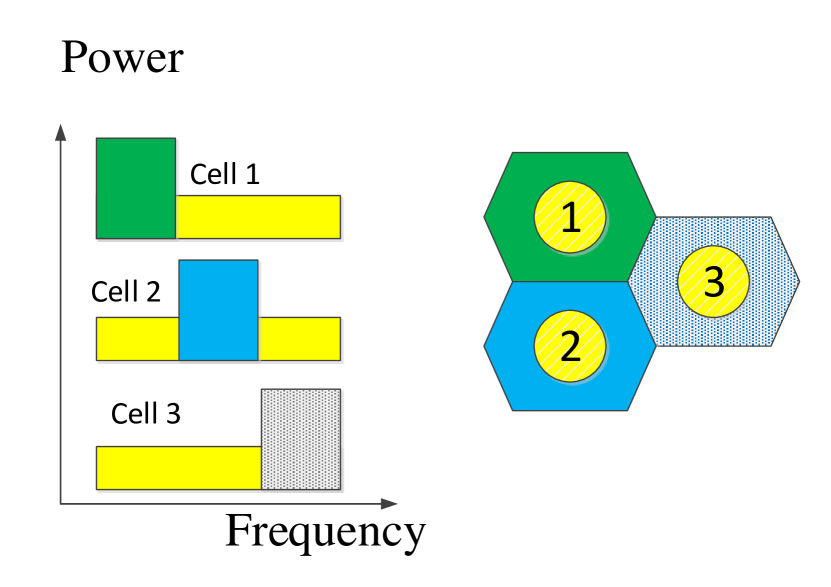
Figure 1: Soft FR with $\Delta=3$

We define $\phi_{i}$ to be transmission power ratio on a cell-edge RB and cell-center RB, i.e. the transmission power on a cell-center and a cell-edge RB in tier $i$ are $P_{i}$ and $\phi_{i}P_{i}$. When the FR factor $\Delta_{i}$ is used, the densities of cells in the tier $i$, that uses the RB $b$ as a cell-center and cell-edge RB, are $\lambda^{(c)}_{i}=\frac{\Delta_{i}-1}{\Delta_{i}}\lambda_{i}$ and $\lambda^{(e)}_{i}=\frac{1}{\Delta_{i}}\lambda_{i}$, respectively.

The intercell interference experienced by a typical CEU, is given by

$$I=\sum\limits_{j=1}^{K}\left\{\sum\limits_{z_{c}\in\theta_{j}^{(c)}}\tau(RB_{jz_{c}}=b)P_{j}g_{jz_{c}}r_{jz_{c}}^{-\alpha_{j}}\right\}\\ +\sum\limits_{j=1}^{K}\left\{\sum\limits_{z_{e}\in\theta_{j}^{(e)}}\tau(RB_{jz_{e}}=b)\phi_{j}P_{j}g_{jz_{e}}r_{jz_{e}}^{-\alpha_{j}}\right\}$$ (3)

in which $\theta_{j}^{(c)}$ and $\theta_{j}^{(e)}$ are the set of interfering BSs transmitting with a cell-center and cell-edge power level in tier $j$; $g_{jz}$ and $r_{jz}$ are the channel power gain and distance from the user to the interfering BS $z$ in the tier $j$; $\tau(RB_{jz_{c}}=b)$ and $\tau(RB_{jz_{e}}=b)$ is the indicator functions that take value 1 if the RB $b$ is occupied as a cell-center or cell-edge RB in cell $z_{c}$ or $z_{e}$.

When Round Robin scheduling is deployed, the expected values of these indicator functions are:

$$\mathbb{E}[\tau(RB_{jz_{c}}=b)]=\frac{M_{j}^{(c)}}{N_{j}^{(c)}}\text{ and }\mathbb{E}[\tau(RB_{jz_{e}}=b)]=\frac{M_{j}^{(e)}}{N_{j}^{(e)}}$$ (4)

For optimisation purposes, the ratio of the number of RBs at a cell-edge and cell-center area is proportional to number of the CEU and CCU [11]. Hence, we define the optimisation factor $\epsilon_{i}$ for the tier $i$ as in Equation 5

$$\frac{M_{j}^{(c)}}{N_{j}^{(c)}}=\frac{M_{j}^{(e)}}{N_{j}^{(c)}}=\epsilon_{j}\quad(\forall 0<i\leq K)$$ (5)

III Coverage probability of a typical cell-edge user

In this section, the coverage probability of a typical user that is served on a cell-edge RB, is considered. The CEU is said under the coverage region if there is at least one tier $i$ among the K tiers such that the received $SINR_{i}(\phi_{i},r_{i})$ from at least one BS in tier $i$ is larger than a coverage threshold $\hat{T_{i}}$.

$$P^{(e)}_{c}=\mathbb{P}\left(\bigcup_{i=1}^{K}SINR_{i}(\phi_{i},r_{i})\geq\hat{T}_{i}\right)=\sum_{i=1}^{K}P_{Ai}P_{i}^{(e)}(\hat{T_{i}},\phi_{i})$$ (6)

where $P^{(e)}_{i}(\hat{T_{i}},\phi_{i})$ is the coverage probability of the user which is associated with the tier $i$ and $P_{Ai}$ is the probability that the user is connected to tier $i$. When the user is under the coverage area, it can successfully decode the received signal. Then, it is clear that the value of $\hat{T_{i}}$ varies depending on the sensitivity of the user equipment.

The received $SINR_{i}(\phi_{i},r_{i})$ from the tier $i$ can be expressed as a function of the distance between the user and its associated BS.

$$SINR_{i}(\phi_{i},r_{i})=\frac{\phi_{i}P_{i}g_{i}r_{i}^{-\alpha_{i}}}{I_{u}+\sigma^{2}}$$ (7)

in which $g_{i}$ and $r_{i}$ is the channel power gain and distance from the user to the serving BS in tier $i$; $\phi_{i}$ is the transmission power ratio that was defined in section II-B; $\sigma^{2}$ is Gaussian noise. The coverage probability in Equation 6 can be rewritten as the following expression

$$P_{c}^{(e)}(\hat{T_{i}},\phi_{i})=\int\limits_{0}^{\infty}\mathbb{P}^{(e)}_{i}(\hat{T_{i}},\phi_{i}|r_{i})f_{R_{i}}(r_{i})dr_{i}$$

$$\quad\quad=\int\limits_{0}^{\infty}\frac{2\pi\lambda_{i}}{P_{Ai}}r_{i}\exp\left(-\pi\sum\limits_{j=1}^{K}\lambda_{j}r_{i}^{\frac{2\alpha_{i}}{\alpha_{j}}}\right)\mathbb{P}^{(e)}_{i}(\hat{T_{i}},\phi_{i}|r_{i})dr_{i}$$ (8)

Hence, to find expression of $P_{c}^{(e)}(\hat{T_{i}},\phi_{i})$, the coverage probability of the CEU at a distance $r_{i}$ from its serving BS, i.e. $\mathbb{P}^{(e)}_{i}(\hat{T_{i}},\phi_{i}|r_{i})$ should be computed first.

Lemma III.1

The coverage probability of the typical cell-edge user at a distance $r_{i}$ from its serving BS in the tier $i$ is given by

$$\mathbb{P}_{i}^{(e)}(\hat{T_{i}},\phi_{i}|r_{i})=\sum\limits_{n=1}^{N_{H}}\frac{\omega_{n}}{\sqrt{\pi}}\exp\left[-\frac{\hat{T_{i}}r_{i}^{\alpha_{i}}}{\gamma(a_{n})}\frac{1}{\phi_{i}SNR_{i}}\right]$$

$$\exp\left[-\pi r_{i}^{2}\sum\limits_{j=1}^{K}\epsilon_{j}\left(\lambda^{(c)}_{j}f_{I}(\hat{T_{i}},\phi_{i},1,i,j)+\lambda^{(e)}_{j}f_{I}(\hat{T_{i}},\phi_{i},\phi_{j},i,j)\right)\right]$$ (9)

where $f_{I}(\hat{T_{i}},\phi_{i},\phi_{j},i,j)=\\$ $\quad\quad\quad\sum\limits_{n_{1}=1}^{N_{H}}\frac{\omega_{n_{1}}}{\sqrt{\pi}}\left[\frac{2\pi C(\hat{T}_{i},\phi_{i})^{\frac{2}{\alpha_{j}}}}{\alpha_{j}\sin\left(\frac{\pi(\alpha_{j}-2)}{\alpha_{j}}\right)}-\sum\limits_{m=1}^{N_{L}}\frac{c_{m}}{2}\frac{C(\hat{T}_{i},\phi_{i})}{c_{m}+\left(\frac{x_{m}+1}{2}\right)^{\alpha_{j}/2}}\right]\text{;}$
${C(\hat{T}_{i},\phi_{i})=\hat{T_{i}}\frac{\gamma(a_{n_{1}})}{\gamma(a_{n})}\frac{\phi_{j}P_{j}}{\phi_{i}P_{i}}r_{i}^{\alpha_{i}-\alpha_{j}}}$ ; $\gamma(a_{n})=10^{(\sqrt{2}\sigma_{z}a_{n}+\mu_{z})/10}$ ;
$\omega_{n}$ and $a_{n}$,$c_{m}$ and $x_{m}$ are are weights and nodes of Gauss-Hermite, Gauss-Legendre rule respectively with order $N_{H}$.

Proof: See Appendix

It is observed from Lemma III.1 that the coverage probability of a typical user is inversely proportional to exponential function of $1/SNR$ and $r^{Î}\textpm_{i}$ for cellular network with $\sigma^{2}>0$. On right-hand side of the equation, the first exponential part corresponds to the transmission SNR which is comparable with the published results and equals 1 in the case of an interference-limited network. Meanwhile, the second exponential part corresponds to the ICI which represents the relationship between one side such as density of BS, transmission ratio and optimisation factor, and other side such as coverage probability. When the FR factor $\Delta=1$, i.e. $\phi_{i}=\phi_{j}\quad\forall i,j$, then the coverage probability expression is comparable with the results in [9, 5].

The main difference between the CEU and CCU is that the CEU is served by the BS transmitting at the high power level while the CCU is served by the BS transmitting with the lower power level. The coverage probability of the typical CCU can be obtained by:

$$\mathbb{P}_{i}^{(c)}(\hat{T_{i}},1|r_{i})=\sum\limits_{n=1}^{N_{H}}\frac{\omega_{n}}{\sqrt{\pi}}\exp\left[-\frac{\hat{T_{i}}r_{i}^{\alpha_{i}}}{\gamma(a_{n})}\frac{1}{SNR_{i}}\right]$$

$$\exp\left[-\pi r_{i}^{2}\sum\limits_{j=1}^{K}\epsilon_{j}\left(\lambda^{(c)}_{j}f_{I}(\hat{T_{i}},1,1,i,j)+\lambda^{(e)}_{j}f_{I}(\hat{T_{i}},1,\phi_{j},i,j)\right)\right]$$ (10)

in which $f_{I}(\hat{T_{i}},1,\phi_{i},i,j)$ and related symbols are defined in Lemma III.1.

Proposition III.2

The average coverage probability of the typical CEU that is randomly located in the network is given by

$$P^{(e)}_{c}=\sum\limits_{i=1}^{K}\sum\limits_{m=1}^{N_{L}}4\pi\lambda_{i}\frac{c_{m}(x_{m}+1)}{(1-x_{m})^{3}}\\ e^{-\pi\sum\limits_{j=1}^{K}\lambda_{j}\left(\frac{x_{m}+1}{1-x_{m}}\right)^{\frac{2\alpha_{i}}{\alpha_{k}}}}\mathbb{P}_{i}^{(e)}\left(\hat{T_{i}},\phi_{i}|r_{m}=\frac{x_{m}+1}{1-x_{m}}\right)$$ (11)

Proof This expression of average coverage probability can be obtained from Equation 8 by using Gauss-Legendre quadrature, i.e. letting $r=\frac{t}{1-t}$.

This closed-form expression for coverage probability of a typical user in Rayleigh-Lognormal fading is simpler and more general than the previous results in [4] which was produced for Rayleigh fading only and a FR factor $\Delta=1$.

Proposition III.3

The average coverage probability of the cell-edge user in an interference-limited network (with no noise) the homogenous network , i.e. $\alpha_{i}=\alpha_{j}$ , $\forall 0<i,j<K$, is given by

$$P {}_{c}^{(e)}(\hat{T_{i}},\phi_{i})=\sum\limits_{i=1}^{K}\sum\limits_{n=1}^{N_{H}}\frac{\omega_{n}}{\sqrt{\pi}}$$

$$\frac{1}{1+\frac{1}{\lambda_{i}}\sum\limits_{j=1}^{K}\epsilon_{j}\left(\lambda^{(c)}_{j}f_{I}(\hat{T_{i}},\phi_{i},1,i,j)+\lambda^{(e)}_{j}f_{I}(\hat{T_{i}},\phi_{i},\phi_{j},i,j)\right)}$$ (12)

Proof When $\sigma^{2}=0$, the desired result can be achieved by evaluating the integral in Equation 8.

This close-form expression is comparable to the corresponding result for Rayleigh fading and FR factor $\Delta=1$ given in [12]. When the number of tiers is one ($K=1$) or the densities of BSs in all tiers are the same, the average coverage probability does not depend on the density of the BS. This means the coverage probability is consistent with the changes the of number of BS [2].

IV Average coverage probability of a typical user

In this section, we derive the average coverage probability of a typical user (called randome user) that is randomly located in a K-tier cellular network and can be either served as a CEU or CCU. Using the same approach that was given in Section III, the average coverage probability is given by

$$P_{c} =\sum\limits_{i=1}^{K}P_{Ai}P_{i}(\hat{T_{i}},\phi_{i})$$ (13)

where $P_{Ai}$ is the probability that the random user is associated with the tier $i$ and $P_{i}(\hat{T_{i}},\phi_{i})$ is the average coverage probability of the random user when it is connected to the tier $i$.

It is noticed $P_{i}(\hat{T_{i}},\phi_{i})$ is obtained by averaging the coverage probability of the user at the distance $r_{i}$, i.e. $\mathbb{P}_{i}(\hat{T_{i}},\phi_{i}|r_{i})$, over the network. Hence,

$$P_{c} =\sum\limits_{i=1}^{K}P_{Ai}\int\limits_{0}^{\infty}\mathbb{P}_{i}(\hat{T_{i}},\phi_{i}|r_{i})f_{R_{i}}(r_{i})dr_{i}$$

$$=\sum\limits_{i=1}^{K}\int\limits_{0}^{\infty}2\pi\lambda_{i}r_{i}\exp\left(-\pi\sum\limits_{j=1}^{K}\lambda_{j}r^{\frac{2\alpha_{i}}{\alpha_{j}}}\right)\mathbb{P}_{i}(\hat{T_{i}},\phi_{i}|r_{i})dr_{i}$$ (14)

where $f_{R_{i}}(r_{i})$ is the PDF of $r_{i}$ that was given in Equation 1.

For a given tier $i$ in a LTE network enabling frequency reuse, a typical user can be served as a CEU (or CCU) when its received SINR, i.e. $SINR_{i}(1,r_{i})$ in Equation 7, is below (or above) the SINR threshold $T_{i}$. If the user is served as a CCU, then it is said to be under the coverage region of the tier $i$ if $SINR_{i}(1,r_{i})$ are larger than both the $SINR$ threshold $T_{i}$ and the coverage threshold $\hat{T}_{i}$. If the user is served as a CEU, then it can be served on different RB and transmission power. Hence, it experience new SINR, i.e. $SINR_{i}^{\prime}(\phi_{i},r_{i})$,. Hence, the user in this case is under the coverage region of the tier $i$ if $SINR_{i}^{\prime}(\phi_{i},r_{i})$ is above the threshold $T_{i}$. Subsequently, the probability $\mathbb{P}_{i}(\hat{T_{i}},\phi_{i}|r_{i})$ of a random user is obtained by

$$\mathbb{P}_{i}(\hat{T_{i}},\phi_{i}|r_{i})= \mathbb{P}(SINR^{\prime}_{i}(1,r_{i})>\hat{T_{i}})\mathbb{P}(SINR_{i}(1,r_{i})>T_{i})$$

$$+\mathbb{P}(SINR^{\prime}(\phi_{i},r_{i})>\hat{T_{i}})\mathbb{P}(SINR_{i}(1,r_{i})<T_{i})$$

$$= \mathbb{P}_{i}^{(c)}(\hat{T_{i}},1|r_{i})\mathbb{P}_{i}^{(c)}(T_{i},1|r_{i})$$

$$+\mathbb{P}_{i}^{(e)}(\hat{T_{i}},\phi_{i}|r_{i})\left[1-\mathbb{P}_{i}^{(c)}(T_{i},1|r_{i})\right]$$ (15)

in which $\mathbb{P}_{i}^{(e)}(\hat{T_{i}},\phi_{i}|r_{i})$ and $\mathbb{P}_{i}^{(c)}(\hat{T_{i}},\phi_{i}|r_{i})$ are given in Equation 9 and 10, respectively.

Using the same approach as in Proposition III.2, the average coverage probability can be obtained by

$$P_{c}=\sum\limits_{i=1}^{K}\sum\limits_{m=1}^{N_{L}}4\pi\lambda_{i}\frac{c_{m}(x_{m}+1)}{(1-x_{m})^{3}}\\ e^{-\pi\sum\limits_{j=1}^{K}\lambda_{j}\left(\frac{x_{m}+1}{1-x_{m}}\right)^{\frac{2\alpha_{i}}{\alpha_{k}}}}\mathbb{P}_{i}\left(\hat{T_{i}},\phi_{i}|r_{m}=\frac{x_{m}+1}{1-x_{m}}\right)$$ (16)

In the case of interference-limited network with a frequency reuse factor $\Delta=1$ is used, i.e. $\phi_{i}=\phi_{j}\forall 0<i,j\leq K$, then the average coverage probability is given by the same approach as in Proposition III.3

$$P_{c}=\sum\limits_{i=1}^{K}\sum\limits_{n=1}^{N_{H}}\frac{\omega_{n}}{\sqrt{\pi}}\frac{1}{1+\frac{1}{\lambda_{i}}\sum\limits_{j=1}^{K}\lambda_{j}\epsilon_{j}f_{I}(\hat{T_{i}},1,1,i,j)}$$ (17)

This closed-form expression of average coverage probability is comparable with the published result in [7]. The average coverage probability only depends on the optimization factor.

V Simulation and Discussion

In this section, the Monte Carlo simulations are used to give a graphical verification of the accuracy of the analytical results presented in Section 4. Furthermore, this section provides more details about the relationship between network performance and the related parameters such as transmission power ratio, optimization factor and coverage threshold.

Since the coverage threshold represents the signal detection probability of the user equipment, it does not depend on the tier in which the user is associated with, i.e. $\hat{T}_{i}=\hat{T}_{j},\quad\forall 0<i,j<K$. To reduce the computation complexity, it is assumed that the path loss exponents at different tiers are the same. The analytical and simulation parameters used in this paper are summarized in Table I.

Parameter	Value
Number of tiers	$K=2$
Density of BSs	Tier 1, $\lambda=0.25$
	Tier 2, $\lambda=0.5$
Transmission power ratio between tiers	$100$
$(P_{1}/P_{2})$
Fading channel	$\mu_{z}=-7.3683$ dB
	$\sigma_{z}=8$ dB
Pathloss exponent	$\alpha_{1}=\alpha_{2}=3.5$

TABLE I: Analytical and simulation parameters

Figure 2 shows variation of the average coverage probability of the CEU (y-axis) versus the coverage threshold in dB (x-axis) from theory and simulation for a number of values of the optimization factors ($\epsilon_{1},\epsilon_{2}$) which represent ratio between the number of users and RBs in each tier.

Figure 2: Coverage probability of a CEU vs. coverage threshold

When the optimization factor increases which means that there is an increase in the number of users, the average coverage probability of the CEU decreases significantly . For example, when the coverage threshold is $\hat{T}_{i}=0$ dB, the coverage probability decreases by 23.6% from 0.4229 to 0.323 when the optimisation factors doubles from ($\epsilon_{1}=0.1,\epsilon_{2}=0.2$) to ($\epsilon_{1}=0.2,\epsilon_{2}=0.6$).

Furthermore, it is observed in Figure 2 that the average coverage probability which is proportional to the detection probability of user equipment. When the sensitivity of user device is improved which means that the user can work with lower SINR (i.e. lower coverage threshold), the probability that the user successfully decodes the received signals increases. Consequently, the performance of this user increases.

In Figure 3, the coverage probability of the CCU, CEU and random user are shown as a function of transmission power ratio .

Figure 3: User coverage probability versus transmission ratio $\phi_{i}$

When the transmission power ratio increases (i.e. an increase in the transmission power on the cell-edge RB), the received signal power for the CEU and the ICI power in the network increases while the power of the received signal of the CCU is kept constant. Hence, as shown in the figure, the coverage probability of the CEU grows moderately, while that of the CCU decreases . For the random user which can be CCU or CEU, the coverage probability increases slightly.

VI Conclusion

In this paper, the coverage probability of a typical user in a multi-tier network experiencing Rayleigh-Lognormal fading is presented through mathematical and numerical analysis. The typical user in this paper can be a CCU, CEU or random user. The main difference between the results in this paper and in other published work is that previous works use either Strict FR or Soft FR with reuse factor $\Delta=1$ . In this paper, FR factor $\Delta>1$ was investigated. The results show that the coverage probability of a typical user is a function of the transmission ratio, FR factor, density of BSs and optimisation factor. Furthermore, the results indicate that there are opposite trends between the performance of the CEU and CCU. Therefore, the optimal problem should consider these factors together.

Appendix A

The coverage probability in Equation 6 can be rewritten as

$$\mathbb{P}^{(e)}_{c}(\hat{T_{i}},\phi_{i}|r_{i})$$

$$=\mathbb{P}(SINR_{i}(\phi_{i},r_{i}))$$

$$=\sum\limits_{n=1}^{N_{H}}\frac{\omega_{n}}{\sqrt{\pi}}\mathbb{E}\left[\exp\left(-\frac{Tr_{i}^{\alpha_{i}}(I_{u}+\sigma^{2})}{\phi_{i}P_{i}\gamma(a_{n})}\right)\right]$$

$$=\sum\limits_{n=1}^{N_{H}}\frac{\omega_{n}}{\sqrt{\pi}}\left[\exp\left(-\frac{Tr_{i}^{\alpha_{i}}}{\gamma(a_{n})}\frac{1}{\phi_{i}SNR_{i}}\right)\mathbb{E}\left\{\exp\left(-\frac{Tr_{i}^{\alpha_{i}}I_{u}}{\phi_{i}P_{i}\gamma(a_{n})}\right)\right\}\right]$$ (18)

in which $SNR_{i}=\frac{P_{i}}{\sigma^{2}}$.

By substituting Equation 3, the expectation can be separated into two elements $\mathbb{E}^{(c)}$ and $\mathbb{E}^{(e)}$.

$$\mathbb{E}\left\{\exp\left(-\frac{Tr_{i}^{\alpha_{i}}}{\phi_{i}P_{i}\gamma(a_{n})}I_{u}\right)\right\}=\mathbb{E}^{(c)}\text{ x }\mathbb{E}^{(e)}$$

in which $\mathbb{E}^{(e)}$ and $\mathbb{E}^{(c)}$ are given in Equation 19

$$\mathbb{E}^{(c)} = \prod\limits_{j=1}^{K}\mathbb{E}\left\{\prod\limits_{z_{c}\in\theta_{j}^{(c)}}\tau(RB_{jz_{c}}=b)\exp\left(-C(\hat{T}_{i},\phi_{i})g_{jz_{c}}\left(\frac{r_{jz_{e}}}{r_{i}}\right)^{-\alpha_{j}}\right)\right\}$$

$$\mathbb{E}^{(e)} = \prod\limits_{j=1}^{K}\mathbb{E}\left\{\prod\limits_{z_{e}\in\theta_{j}^{(e)}}\tau(RB_{jz_{e}}=b)\exp\left(-C(\hat{T}_{i},\phi_{i})g_{jz_{e}}\left(\frac{r_{jz_{e}}}{r_{i}}\right)^{-\alpha_{j}}\right)\right\}$$ (19)

$$\text{in which}\quad C(\hat{T}_{i},\phi_{i})=\hat{T}_{i}\frac{\gamma(a_{n_{1}})}{\gamma(a_{n})}\frac{\phi_{j}P_{j}}{\phi_{i}P_{i}}r_{i}^{\alpha_{i}-\alpha_{j}}.$$

Evaluating the second group product $\mathbb{E}^{(e)}$, we have

$$\mathbb{E}^{(e)}=\prod\limits_{j=1}^{K}\mathbb{E}\left\{\prod\limits_{z_{e}\in\theta_{j}^{(e)}}\epsilon_{j}\\ \quad\quad\quad\quad\quad\quad\quad\mathbb{E}_{g_{jz}}\left[\exp\left(-C(\hat{T}_{i},\phi_{i})g_{jz_{e}}\left(\frac{r_{jz_{e}}}{r_{i}}\right)^{-\alpha_{j}}\right)\right]\right\}$$

Since $g_{jz_{c}}$ is Rayleigh-Lognormal fading channel then

$$= \prod\limits_{j=1}^{K}\mathbb{E}\left\{\prod\limits_{z_{e}\in\theta_{j}^{(c)}}\epsilon_{j}\sum\limits_{n_{1}=1}^{N_{H}}\frac{\omega_{n_{1}}}{\sqrt{\pi}}\frac{1}{1+C(\hat{T}_{i},\phi_{i})\left(\frac{r_{jz_{e}}}{r_{i}}\right)^{-\alpha_{j}}}\right\}$$

Each element of this product can be evaluated by using the properties of PPP generating function, Gamma function and Gauss-Legendre approximation quadrature shown in [7], then the expectation $\mathbb{E}^{(e)}$ equals

$$\mathbb{E}^{(e)}=\exp\left(-\pi\lambda^{(e)}_{j}r_{i}^{2}\sum\limits_{j=1}^{K}\epsilon_{j}f_{I}(\hat{T_{i}},\phi_{i},\phi_{j},i,j)\right)$$ (20)

in which

$$f_{I}(\hat{T_{i}},\phi_{i},\phi_{j},i,j)=\sum\limits_{n_{1}=1}^{N_{H}}\frac{\omega_{n_{1}}}{\sqrt{\pi}}\left(\frac{2\pi C(\hat{T}_{i},\phi_{i})^{\frac{2}{\alpha_{j}}}}{\alpha_{j}\sin\left(\frac{\pi(\alpha_{j}-2)}{\alpha_{j}}\right)}\\ -\sum\limits_{m=1}^{N_{H}}\frac{c_{m}}{2}\frac{C(\hat{T}_{i},\phi_{i})}{c_{m}+\left(\frac{x_{m}+1}{2}\right)^{\alpha_{j}/2}}\right)$$ (21)

where $c_{m}$ and $x_{m}$ are are weights and nodes of Gauss-Legendre rule with order $N_{L}$. Similarly, $\mathbb{E}^{(c)}$ is achieved by

$$\mathbb{E}^{(c)}=\exp\left(-\pi\lambda_{j}^{(c)}r_{i}^{2}\sum\limits_{j=1}^{K}\epsilon_{j}\phi_{j}f_{I}(T,\phi_{i},1,i,j)\right)$$ (22)

Substituting Equation 20 and 22 into Equation 18, the Theorem is proved.

References

- [1] Soft Frequency Reuse Scheme for UTRAN LTE, 3GPP Project Document Std. R1-050 507, Huawei,2005.
- [2] J. G. Andrews, F. Baccelli, and R. K. Ganti, “A new tractable model for cellular coverage,” in Communication, Control, and Computing (Allerton), 2010 48th Annual Allerton Conference on, Conference Proceedings, pp. 1204–1211.
- [3] A. G. J. G. A. Thomas David Novlan, Radha Krishna Ganti, “Analytical evaluation of fractional frequency reuse for ofdma cellular networks,” IEEE TRANSACTIONS ON WIRELESS COMMUNICATIONS, vol. 10, pp. 4294–4305, 2011.
- [4] H. S. Dhillon, R. K. Ganti, F. Baccelli, and J. G. Andrews, “Modeling and analysis of k-tier downlink heterogeneous cellular networks,” Selected Areas in Communications, IEEE Journal on, vol. 30, no. 3, pp. 550–560, 2012.
- [5] H.-S. Jo, Y. J. Sang, P. Xia, and J. Andrews, “Heterogeneous cellular networks with flexible cell association: A comprehensive downlink sinr analysis,” Wireless Communications, IEEE Transactions on, vol. 11, no. 10, pp. 3484–3495, October 2012.
- [6] W. Bao and B. Liang, “Structured spectrum allocation and user association in heterogeneous cellular networks,” in INFOCOM, 2014 Proceedings IEEE, April 2014, pp. 1069–1077.
- [7] S. C. Lam and K. Sandrasegaran, “A closed-form expression for coverage probability of random cellular network in composite rayleigh-lognormal fading channels,” in Accepted for Publication at International Telecommunication Networks and Applications Conference (ITNAC), November, 2015.
- [8] H. P. Keeler, B. Blaszczyszyn, and M. K. Karray, “Sinr-based k-coverage probability in cellular networks with arbitrary shadowing,” in Information Theory Proceedings (ISIT), 2013 IEEE International Symposium on, Conference Proceedings, pp. 1167–1171.
- [9] S. C. Lam, K. S. Sandrasegaran, and Q. T. Nguyen, “Performance of soft frequency reuse in random cellular networks in rayleigh-lognormal fading channels,” in Accepted for publication at APCC 2016, Indonesia.
- [10] M. Dinh Thi Thai, C. Lam Sinh, T. Nguyen Quoc, and N. Dinh-Thong, “Ber of qpsk using mrc reception in a composite fading environment,” in Communications and Information Technologies (ISCIT), 2012 International Symposium on, Conference Proceedings, pp. 486–491.
- [11] L. Chen and D. Yuan, “Generalized frequency reuse schemes for ofdma networks: Optimization and comparison,” in Vehicular Technology Conference (VTC 2010-Spring), 2010 IEEE 71st, May 2010, pp. 1–5.
- [12] T. O. He Zhuang, “A model based on poisson point process for downlink k tiers fractional frequency reuse heterogeneous networks,” Physical Communication, vol. Volume 13, Part B, no. Special Issue on Heterogeneous and Small Cell Networks, p. 3–12, 2014.