Enhanced diffusion and anomalous transport of magnetic colloids driven above a two-state flashing potential

Abstract

We combine experiment and theory to investigate the diffusive and subdiffusive dynamics of paramagnetic colloids driven above a two-state flashing potential. The magnetic potential was realized by periodically modulating the stray field of a magnetic bubble lattice in a uniaxial ferrite garnet film. At large amplitudes $H_{0}$ of the driving field, the dynamics of particles resembles an ordinary random walk with a frequency-dependent diffusion coefficient. However, subdiffusive and oscillatory dynamics at short time scales is observed when decreasing $H_{0}$. We present a persistent random walk model to elucidate the underlying mechanism of motion, and perform numerical simulations to demonstrate that the anomalous motion originates from the dynamic disorder in the structure of the magnetic lattice, induced by slightly irregular shape of bubbles.

I Introduction

Transport and diffusion of microscopic particles through periodic potentials is a rich field of research from both fundamental and technological points of view Reimann (2002); Hanggi and Marchesoni (2009). Investigation of the particle motion along ordered Reimann (2002) or disordered Sancho et al. (2004); Hanes et al. (2012) energy landscapes helps to better understand the dynamics in more complex situations, such as Abrikosov Villegas et al. (2003); de Vondel et al. (2005) and Josephson vortices in superconductors Majer et al. (2003); Ustinov et al. (2004), cell migration Mahmud et al. (2009), or transport of molecular motors Julicher et al. (1997). Moreover, a periodic potential can be used to perform precise particle sorting and fractionation Korda et al. (2002); MacDonald et al. (2003); Huang et al. (2004); Lacasta et al. (2005); Tierno et al. (2008), thus, being of significant impact in diverse fields in analytical science and engineering which make use of microfluidic devices. Colloidal systems provide an ideal opportunity to investigate different transport scenarios, because of having particle sizes in the visible wavelength range and dynamical time scales which are experimentally accessible. In order to force colloidal particles to move along periodic or random trajectories, static potentials can be readily realized by using optical Dalle-Ferrier et al. (2011), magnetic Tierno et al. (2007), or electric fields Pertsinidis and Ling (2008). Dynamic landscapes (obtained by periodically or randomly modulating the potential) are a subject of growing interest since a rich dynamics can be induced due to the presence of competing time scales. Moreover, flashing potentials where static landscapes are modulated in time, are usually employed to study molecular systems Astumian and Bier (1994); Prost et al. (1994); Cao et al. (2004) or as an efficient way to transport and fractionate Brownian species Faucheux et al. (1995); Libál et al. (2006).

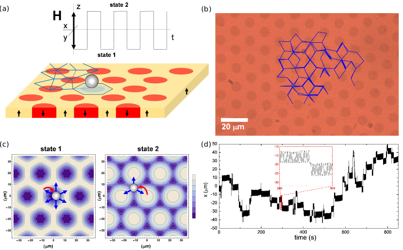
Figure 1: (a) Schematic showing a paramagnetic particle driven above a magnetic bubble lattice by a square wave magnetic field $\bf H$. One Wigner-Seitz cell is shaded in blue. (b) Microscope image of a bubble lattice with a superimposed trajectory of one particle (blue lines) for $\omega{=}12.6\,{\rm rad\,s^{-1}}$ and $H_{0}{=}0.14\,{\rm M_{s}}$. (c) Contour plots of the normalized magnetostatic energy $E/k_{B}T$ of one particle above the bubble lattice at two different times separated by half a period. Energy maxima (minima) are colored in white (blue). The blue arrows indicate the possible paths the particle can undertake in the next jump. The red arrows show the path undertaken by the particle to reach the energy minimum. (d) Time evolution of the $x-$coordinate of one paramagnetic particle subjected to an external square wave field with $H_{0}{=}0.14\,{\rm M_{s}}$ and $\omega{=}15.7\,{\rm rad\,s^{-1}}$. The red inset zooms in one piece of the trajectory.

Here we present a combined experimental and theoretical study focused on the dynamics of microscale particles driven above a flashing magnetic potential. This potential is generated by periodically modulating the energy landscape created by an array of magnetic bubbles. As it was previously reported Tierno et al. (2009), this experimental system is able to generate different dynamical states depending on the applied field parameters, such as frequency or amplitude of the external field. In particular we report the observation of enhanced diffusive dynamics at high field strength $H_{0}$, while the motion at lower $H_{0}$ is subdiffusive with a crossover to normal diffusion at long times. At low values of $H_{0}$, the lattice structure is slightly disordered during the switching of the magnetic field direction. The resulting randomness is dynamic, i.e. not reproducible after a cycle of external drive, and enhances with decreasing $H_{0}$. By means of numerical simulations we verify that in the presence of lattice disorder, the particles frequently experience oscillatory motion in local traps. The back and forth motion of particle in local traps happens more frequently as the dynamic disorder in the structure of the magnetic lattice increases. The trapping events change the statistics of the turning angles of the particle from an isotropic distribution (limited to the directions allowed by the lattice structure) to an anisotropic one with a tendency towards backward directions. Using a persistent random walk model, we show that anomalous diffusion arises when the turning-angle distribution of a random walker is asymmetric along the arrival direction. When the walker has the tendency towards backward directions, the resulting antipersistent motion is subdiffusive or even strongly oscillatory at short time scales. However, the walker has a finite range memory of the successive step orientations, i.e. the direction gets randomized after long times and the asymptotic behavior is ordinary diffusion with a smaller long-term diffusion coefficient compared to an ordinary random walk. We obtain good agreement between the analytical predictions, simulations, and experiments.

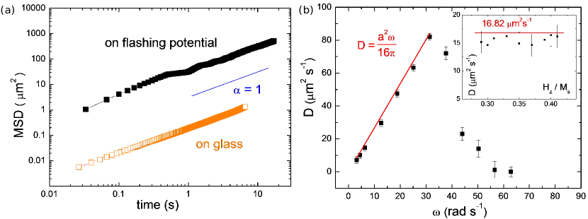
Figure 2: (a) Mean squared displacement versus time for a paramagnetic colloid above a glass substrate (open squares) and above a two-state flashing potential (solid squares), under a field with amplitude $H_{0}{=}0.37\,{\rm M_{s}}$ and angular frequency $\omega{=}6.3\,\,{\rm rad\,s^{-1}}$. (b) Effective diffusion coefficient $D$ vs angular frequency $\omega$ for a colloidal particle driven by an applied field with $H_{0}{=}0.37\,{\rm M_{s}}$. The solid line denotes the relationship $D{=}\frac{a^{2}\omega}{16\pi}$. The inset shows $D$ vs $H_{0}$, at a constant angular frequency of $\omega{=}6.3\,{\rm rad\,s^{-1}}$.

The paper is organized in the following manner: First we introduce the setup in Sec. II. Section III contains the experimental results obtained at different field parameters. In Sec. IV, the results of numerical simulations for transport in the presence of dynamic disorder are discussed and compared with the corresponding experimental data. The motion of particles is modeled at the level of individual steps via an antipersistent random walk approach in Sec. V, and finally Sec. VI concludes the paper.

II Experimental Setup

A schematic illustrating the experimental system is shown in Fig. 1(a). The colloidal particles used are polystyrene paramagnetic microspheres (Dynabeads M-270, Invitrogen) having diameter $d{=}2.8\,{\rm\mu m}$ and magnetic volume susceptibility $\chi{\sim}0.4$. The particles are diluted in high-deionized water and let sediment above the periodic potential generated by a bismuth-substituted ferrite garnet film (FGF). The FGF has composition Y_2.5Bi_0.5Fe_5-qGa_qO₁₂ ($q{\in}[0.5,1]$) and was previously grown by dipping liquid phase epithaxy on a $0.5mm$ thick gadolinium gallium garnet substrate Tierno et al. (2009). The film has thickness $\sim{\rm 4\mu m}$ and saturation magnetization $M_{s}{=}1.7{\times}10^{4}\,{\rm Am^{-1}}$. In the absence of external field, this FGF is characterized by a labyrinth of stripe domains with alternating magnetization and a spatial periodicity of $\lambda=9.8\,\mu m$. This pattern is converted into a periodic lattice of cylindrical magnetic domains by using high frequency magnetic field pulses applied perpendicular to the film, with amplitude $H_{0}$ and oscillating at angular frequency $\omega$. As shown in Fig. 1, the cylindrical domains, also known as “magnetic bubbles” Eschenfelder (1980), are ferromagnetic domains with radius $R{=}4.2\,{\rm\mu m}$, having the same magnetization direction and arranged into a triangular lattice with lattice constant $a{=}11.6\,{\rm\mu m}$. We can visualize both the magnetic domains in the film and the particles using polarization microscopy, due to the polar Faraday effect.

The external oscillating field is obtained by connecting a coil perpendicular to the film plane ($z$-direction) with a wave generator (TTi - TGA1244) feeding a power amplifier (IMG STA-800). The custom-made coil was mounted on the stage of a polarization light microscope (Nikon, E400) equipped with a $100\times$, $1.3$NA objective and a $0.45$ TV lens. The movements of the particles are recorded at $60$ fps for $\sim 30$ min with a $\text{b}{/}\text{w}$ CCD camera inside an observation area of $179{\times}231\,{\rm\mu m^{2}}$. We then use particle tracking routines Crocker and Grier (1996) to extract the particle trajectories and later calculate correlation functions.

III Particle dynamics in a flashing potential

Once deposited above the garnet film, the paramagnetic particles pin to the Bloch walls, which are located at the boundary of the magnetic bubbles. To generate a two-state flashing potential we apply to the FGF film a square-wave modulation of type

$${\bf H}=H_{0}\,\mathrm{sgn}\big{(}\sin{(\omega t)}\big{)}{\bf e}_{z}\,,$$ (1)

where $H_{0}$ is the field amplitude, $\omega$ the angular frequency, and $\mathrm{sgn}(x)$ denotes the sign function. The applied field periodically changes the radii of the bubbles in the FGF, increasing (decreasing) the size of the bubbles when it is parallel (resp. antiparallel) to their magnetization direction, thus alternating between two distinct states. One can understand the effect of the applied field on the energy landscape by calculating the magnetostatic potential at the particle elevation Soba et al. (2008) see Fig. 1(c). In particular, when the field expands the bubbles (state 1), the energy displays a paraboloid-like minimum within the magnetic domains. Thus, the magnetic colloids are attracted towards the center of the bubble domains. When the field has opposite polarity, it shrinks the size of the bubbles and enlarges the interstitial region (state 2). In this situation, the magnetostatic potential features six regions of energy minima with triangular shape at the vertices of the Wigner-Seitz cell around each bubble.

As a consequence, during the transition 1${\rightarrow}$2, a particle can jump to $6$ possible places [Fig. 1(c), left], while in the transition 2${\rightarrow}$1 the possibilities reduce to $3$ [Fig. 1(c), right]. Since we apply a field perpendicular to the sample plane (no tilt), the potential preserves its spatial symmetry, i.e. there is no net drift motion as it was induced in Ref. [17] by using a precessing field. We analyze the particle dynamics by measuring the mean squared displacement via a temporal moving average $\text{MSD}(t){=}\langle\big{(}x(t{+}t^{\prime}){-}x(t^{\prime})\big{)}^{2}\rangle{\sim}t^{\alpha}$. Here, $x$ denotes the position of the particle projected along one of the crystallographic axes and $\alpha$ the exponent of the power-law which is used to distinguish the diffusive ($\alpha{=}1$) from subdiffusive ($\alpha{<}1$) dynamics. In our system we observe both types of dynamics, which are discussed in the following subsections.

III.1 Diffusive dynamics

In Fig. 2(a) we compare the MSD for a paramagnetic colloid freely diffusing on a glass plane in the absence of FGF film and the one which is strongly driven by the flashing potential. Both cases exhibit a normal diffusion but with different diffusion coefficients. From the experimental data of the MSD, the effective diffusion coefficient of the particle can be estimated as $D{=}\lim\limits_{t\rightarrow\infty}\text{MSD}(t)/2dt$, with $d$ being the spatial dimension (Here $d{=}1$ since the data is projected along one of the crystallographic axes). We find that $D$ in the presence of the flashing potential ($D{=}14.6\,{\rm\mu m^{2}\,s^{-1}}$) is enhanced by nearly two orders of magnitude with respect to the one on a glass plate ($D{=}0.14\,{\rm\mu m^{2}\,s^{-1}}$). In this regime of motion, which is observed for field amplitudes $H_{0}\in[0.28,0.42]\,{\rm M_{s}}$ and frequency $\omega{<}35\,{\rm rad\,s^{-1}}$, the particle moves from one domain to the next without performing continuous oscillation around a single site, thus, it performs an ordinary random walk on a triangular lattice. The step length $l$ of the walker can be estimated to be given by one side of the Wigner-Seitz cell, i.e. $\ell{=}\frac{a}{2}{=}5.8\,{\rm\mu m}$, and the component of the MSD along a crystallographic axis equals $\langle x^{2}\rangle{=}(\frac{\ell}{\sqrt{2}})^{2}{=}\frac{\ell^{2}}{2}$. Each step takes a half-period of the magnetic field pulse, thus, the duration of each step is given by $t_{s}{=}\frac{T}{2}{=}\frac{\pi}{\omega}$. One thus obtain the diffusion coefficient as Machta and Zwanzig (1983); Klages and Dellago (2000) $D{=}\frac{\langle x^{2}\rangle}{2t_{s}}{=}\frac{l^{2}}{4t_{s}}{=}\frac{a^{2}\omega}{16\pi}$. We confirm this relation in Fig. 2(b) by measuring $D$ versus the frequency and amplitude of the applied field. While $D$ increases linearly with frequency, it decrease rapidly beyond $\omega{\sim}30\,\text{rad}\,s^{-1}$ since the overdamped particle is unable to follow the fast vibrations of the potential, and reduces significantly its diffusive dynamics. In contrast to frequency, $D$ is almost independent of the amplitude of the applied field, since the lattice constant of the magnetic bubble array does not change significantly for amplitude $H_{0}{<}0.5\,{\rm M_{s}}$ Tierno et al. (2007). Beyond this value, however, the magnetic bubble lattice starts melting and transport of the particles is not possible anymore.

III.2 Subdiffusive dynamics

Our experimental setup allows us to independently vary both the amplitude $H_{0}$ and the frequency $\omega$ of the driving field. At strong fields ($H_{0}{>}0.28\,{\rm M_{s}}$), the particle jumps between nearest bubbles with an equal probability to choose any of the possible movements, thus, performs a normal random walk on a triangular lattice ($\alpha{\simeq}1$ on all time scales). In contrast, when the field is weak ($H_{0}{<}0.09\,{\rm M_{s}}$), the landscape deformations induced by the applied field are small and the particle is unable to leave the magnetic bubble. The corresponding particle trajectory is composed of simple oscillations between the center of one bubble and one of its six surrounding energy minima. In such a pure localization the MSD saturates rapidly, leading to an exponent $\alpha{\simeq}0$. In the intermediate regime of amplitudes, i.e. $H_{0}{\in}[0.09,0.28]\,{\rm M_{s}}$, we observe a subdiffusive dynamics at short time scales with a crossover to normal diffusion at long times. Figure 3 shows several examples of the temporal evolution of MSD for different values of $H_{0}$ and $\omega$. The initial anomalous exponent varies between $0$ and $1$ depending on the strength $H_{0}$ of the applied magnetic field. While in a previous work Tierno et al. (2009) it was found a stable subdiffusive exponent $\alpha{=}0.5$ for $H_{0}=0.13\,{\rm M_{s}}$ and at different frequencies, the value of $\alpha$ may vary by changing the amplitude of the switching field. To see this more clearly, we rescale both axes in such a way that the asymptotic diffusive regimes of the curves collapse on a master curve (see inset). This can be achieved if the MSD is scaled by $\frac{4\ell}{v}D_{\text{asymp}}$ ($D_{\text{asymp}}$ being the long-term diffusion coefficient, $\ell$ the step size, and $v$ the velocity of the particle), and the time axis is scaled by $\frac{\pi}{\omega}$ to synchronize the oscillations. Only the samples which reach the long-term diffusion limit within our experimental time window are considered. With increasing $H_{0}$, the curves are initially more steep and converge faster to the asymptotic limit.

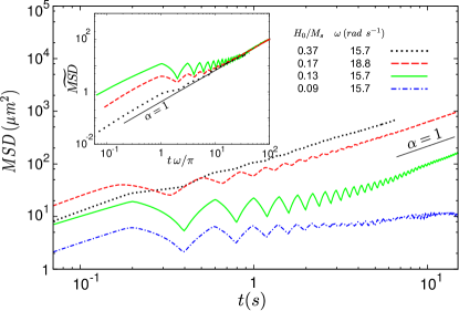
Figure 3: Mean squared displacement versus time for a paramagnetic colloid subjected to a two-state flashing potential for different values of amplitude $H_{0}$ and frequency $\omega$ of the applied magnetic field. Inset: The dimensionless mean squared displacement $\widetilde{\text{MSD}}=\text{MSD}/(\frac{4\ell}{v}D_{\text{asymp}})$ versus the scaled time $t\omega/\pi$.

Indeed, the lattice structure is slightly disordered at weak fields, because of the non-uniform deformations of the magnetic bubbles during their periodic expansion/contraction. These deformations arise from the presence of pinning sites in the film and other inhomogeneities (such as dislocations or magnetic and non-magnetic inclusions present in the FGF crystal). These defects exert an influence on the Bloch walls analogous to the action of a frictional force against the motion of the walls Bar’yakhtar et al. (1977). Furthermore, when the field is applied, the magnetic bubbles interact via long range dipolar forces Seshadri and Westervelt (1992) and small deviations from the 2D projected circular shape induce a slight distortion on the triangular lattice. For the fields used in our experiments, these distortions are not strong enough to create permanent defects in the film (such as disclinations or dislocations), but slightly vary the lattice spacing from place to place. Thus, the spatial structure of the lattice is not perfectly symmetric in practice. In the presence of disorder, the particle may oscillate around each site before it moves to the next domain (see Fig. 1(d) for an example of such movements), which leads to subdiffusive dynamics at short time scales. However, this bias decays with time and the directions of the particle motion become asymptotically randomized, leading to diffusive dynamics at long times. With decreasing $H_{0}$, the lattice disorder and thus the frequency of trapping events enhances, which further decreases the initial anomalous exponent from one (ordinary random walk) towards zero (pure localization).

The frequency $\omega$ of the driving field does not affect the MDS behavior; it only rescales the time because the time step is given by $t_{s}{=}\frac{\pi}{\omega}$. Thus, it can be understood why the crossover time to asymptotic diffusion was found to follow a power-law $\tau_{c}{\sim}\omega^{-1}$ with $\omega$ Tierno et al. (2009).

IV Simulation results

In the previous section we explained the origin of the disorder in the lattice structure during switching of the magnetic field. As a result, the particle spends part of the time in local traps, where it experiences an oscillatory movement. In a back and forth motion, the particle chooses nearly backward directions when it turns. Therefore, the turning-angle distribution $f(\phi)$ changes from an isotropic one for ordinary random walk on the lattice (limited to the allowed directions by the lattice structure) to an anisotropic one with a tendency towards backward directions with respect to the current direction of motion. In the extreme limit of pure localization (remaining permanently in a trap), $f(\phi)$ is a delta function at $\phi{=}\pi$. Such anisotropic turning-angle distributions slow down the spread of colloids on the lattice and cause subdiffusion at short times. The structural irregularities in the magnetic bubble lattice are more pronounced at smaller values of $H_{0}$. Hence, with decreasing $H_{0}$ the chance of trapping events increases and the resulting $f(\phi)$ becomes more anisotropic, which decreases the initial anomalous exponent.

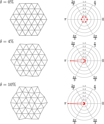
Figure 4: (left) Schematic drawing of the disordered lattice and (right) a polar representation of the corresponding turning-angle distribution $f(\phi)$ after $10000$ steps in simulations for different values of the lattice disorder $\delta$.

In order to ensure that the lattice disorder causes asymmetric turning-angle distribution $f(\phi)$ and subdiffusive dynamics, we perform Molecular Dynamics simulations of motion on a dynamic disordered triangular lattice of synchronous flashing magnetic poles. To obtain smooth particle trajectories and a detailed time evolution of the MSD, in particular to monitor the oscillatory dynamics at short times, MD simulations are advantageous compared to other possible methods such as Monte Carlo simulations. The simulation cell consists of nearly 3000 magnetic poles and a colloidal particle which is initially released near the center of the system to avoid boundary effects. We impose periodic boundary conditions, and consider in-plane magnetic interactions between the immobile poles and the magnetic colloid. The time step of our in-house code is chosen to be $\Delta\,t{=}1{\times}10^{-4}$s, so that the time $t_{s}{=}\frac{\pi}{\omega}$ between two successive switching of the field direction is resolved into more than 1000 time steps. An explicit Euler update scheme is used for integration and the simulations run until the crossover to asymptotic diffusion occurs or the total number of time steps exceeds $5{\times}10^{5}$.

The structural disorder is effectively introduced by random displacements of magnetic poles from their ordered lattice positions. The strength of disorder can be quantified by the parameter $\delta$, denoting the maximum possible displacement of each magnetic pole from its ordered lattice position. We randomly choose the position of each node within a circle of radius $L{\cdot}\delta$ around the corresponding node of the ordered triangular lattice, where $L$ denotes the size of the Wigner-Seitz cell. The dynamic disorder is generated by instantaneous random rearrangements of the poles at each switching event. Thus, the poles move to new positions where they stay immobile until the next switching event. The new random position of each pole remains within the allowed range around the original position of the corresponding ordered lattice node. This way we keep the deviations dynamic but smaller than $\delta{\cdot}L$ in all cases.

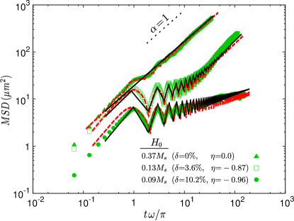
Figure 5: MSD versus time, obtained from experiments (green symbols), simulations (red dashed lines), and the persistent random walk model via Eq. (7) (black solid lines). The experimental data at $\omega{=}15.7\,{\rm rad\,s^{-1}}$ and various amplitudes $H_{0}$ are compared to the best fits obtained by tunning a single fitting parameter (i.e. the lattice disorder $\delta$ in simulations, or the turning-angle anisotropy $\eta$ in the analytical model). The best-fitting parameters for each value of $H_{0}$ are given.

We analyze the particle trajectory for different values of $\delta$. As shown in Fig. 4, with increasing $\delta$ the distortion of the lattice is more pronounced, thus, the particle experiences oscillatory movements in traps more frequently and for longer times, which increases the asymmetry of the turning-angle distribution $f(\phi)$. By tunning $\delta$, as a single free parameter in our simulations, a remarkable agreement with the experimental MSD data is achieved (see Fig. 5). Moreover, by smoothening the MSD curves obtained from simulations, we fit the initial slope of the curves to $\text{MSD}(t){\sim}t^{\alpha}$ to get the anomalous exponent at short times. The results shown in Fig. 6 reveal that with increasing the amount of structural disorder, the slope gradually decreases from $\alpha{=}1$ for normal diffusion towards $\alpha{=}0$ corresponding to pure localization. The growth of MSD is extremely slow for $\delta{\geq}25\%$, in accord with the experimental data at weak fields $H_{0}{<}0.09\,{\rm M_{s}}$.

V Persistent random walk model

So far, we have shown that for small amplitudes of the external field the turning-angle distribution $f(\phi)$ is asymmetric, which is accompanied by a subdiffusive dynamics at short times. In this section, we theoretically consider the particle motion at the level of individual steps and show how the asymmetry of $f(\phi)$ with a tendency towards backward directions leads to subdiffusion. It was demonstrated in a previous work Tierno et al. (2009) that the statistical properties of the subdiffusive motion could be captured by the “random walk on random walk” model Kehr and Kutner (1982) (RWRW), which is a simple example of stochastic motion in a complex environment. In the RWRW model, the walker performs an ordinary random walk on an environment which is constructed by an ordinary random walk process as well. While this model showed a quantitative agreement with the experiments for certain field parameters Tierno et al. (2009), the randomness of the environment indeed varies depending on the choice of $H_{0}$. Thus a more general theoretical framework is needed in order to capture the particle dynamics in the subdiffusive regime for all field parameters. Here, we look at the individual steps of the random walker and present an antipersistent model which enables us to reproduce fine details of motion such as the oscillatory dynamics observed at smaller values of $H_{0}$. Persistent random walk models Furth (1917); Taylor (1922); Haus and Kehr (1987); Weiss (1994) have been used to describe e.g. stochastic transport on cytoskeletal filaments Shaebani et al. (2014); Sadjadi et al. (2015), self-propulsion subject to fluctuations Howse et al. (2007); Peruani and Morelli (2007), or diffusive transport of light in foams and granular media Sadjadi et al. (2008); Sadjadi and Miri (2011). In the following, the asymmetry of $f(\phi)$ is quantified with $\eta{\equiv}\langle\cos\phi\rangle$, which varies from $0$ for an isotropic distribution $f(\phi){=}\frac{1}{2\pi}$ to $-1$ for an extremely asymmetric distribution $f(\phi){=}\delta(\phi{-}\pi)$. We obtain analytical expressions for the time evolution of the MSD, the crossover time to asymptotic diffusion, and the long-term diffusion coefficient in terms of the control parameter $\eta$ and compare the analytical predictions with the experimental data.

Figure 6: The anomalous exponent $\alpha$ at short times (after smoothening the MSD curves) in terms of the structural disorder $\delta$ of the lattice.

We consider a random walk in 2D, with uncorrelated step sizes $\ell$ which are obtained from an arbitrary distribution $g(\ell)$. The successive step orientations are however correlated such that a new orientation is obtained from a turning-angle distribution $f(\phi)$ along the previous direction of motion (see Fig. 7). While an isotropic $f(\phi)$ leads to a normal diffusion, introducing anisotropy along the arrival direction induces persistency and results in an anomalous transport on short time scales. The choices of $f(\phi)$ which encourage the walker towards backward (forward) directions lead to subdiffusion (superdiffusion). Such an approach had been used e.g. in the context of cell migration along surfaces Nossal and Weiss (1974), animal movement Kareiva and Shigesada (1983), and dynamics of polymer chains Flory (1969); Freed (1987). Starting from the origin, let us assume that the first direction of motion is chosen randomly, i.e. the initial condition is $P(\alpha_{1}){=}\frac{1}{2\pi}$. The $x$-coordinate of walker after $n$ steps can be obtained by projecting each step along the $x$-axis

$$x=\sum_{i{=}1}^{n}x_{i}=\sum_{i{=}1}^{n}\ell_{i}\cos\alpha_{i},$$ (2)

where $\alpha_{i}{=}\alpha_{1}{+}\phi_{2}{+}\cdot\cdot\cdot{+}\phi_{i}$. For simplicity, in the following we consider a constant step length $g(\ell){=}\delta(\ell{-}\langle\ell\rangle)$ and $f(\phi)$ distributions with left-right symmetry. The first moment of displacement $\langle x\rangle$ then reads

$$\langle x\rangle= \langle\ell\rangle\langle\sum_{i{=}1}^{n}\cos\alpha_{i}\rangle=\langle\ell\rangle\sum_{i{=}1}^{n}\int_{-\pi}^{\pi}\!\!\!\!\!\!d\phi_{i}f(\phi_{i})\cdot\cdot\cdot\!\!\int_{-\pi}^{\pi}\!\!\!\!\!\!d\phi_{2}f(\phi_{2})$$ (3)

$$\times\int_{-\pi}^{\pi}\!\!d\alpha_{1}P(\alpha_{1})\cos(\alpha_{1}{+}\phi_{2}{+}\cdot\cdot\cdot\phi_{i})=0,$$

since the integral over $\alpha_{1}$ vanishes. Here $\langle\cdot\cdot\cdot\rangle$ denotes an ensemble average. The second moment of displacement is given by Nossal and Weiss (1974); Kareiva and Shigesada (1983); Flory (1969); Freed (1987)

$$\langle x^{2}\rangle =\langle\sum_{i{=}1}^{n}\sum_{j{=}1}^{n}x_{i}x_{j}\rangle=\langle\sum_{i{=}1}^{n}x_{i}^{2}+2\sum_{i{>}j}x_{i}x_{j}\rangle$$ (4)

$$=\sum_{i{=}1}^{n}\langle x_{i}^{2}\rangle+2\sum_{i{=}1}^{n}\sum_{j{=}1}^{i{-}1}\langle x_{i}x_{j}\rangle.$$

Similar to Eq. (3), the first term can be obtained as

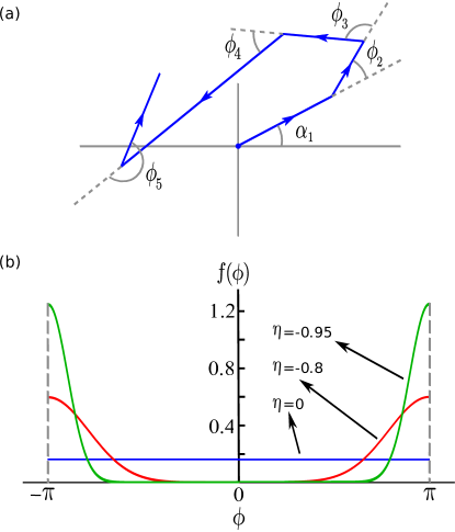
Figure 7: (a) Trajectory of the walker during a few successive steps. (b) Examples of the turning-angle distribution $f(\phi)$ for different values of the asymmetry measure $\eta$.

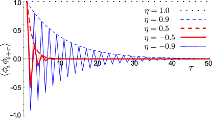
Figure 8: The normalized auto-correlation function $\langle\phi_{i}\phi_{i{+}\tau}\rangle$ versus time for different values of $\eta$. Positive (negative) $\eta$ corresponds to persistent (antipersistent) motion. $\eta{=}1$ denotes a ballistic motion without any turning.

$$\langle x_{i}^{2}\rangle= \langle\ell^{2}\rangle\int_{-\pi}^{\pi}\!\!\!\!\!\!d\phi_{i}f(\phi_{i})\cdot\cdot\cdot\!\!\int_{-\pi}^{\pi}\!\!\!\!\!\!d\phi_{2}f(\phi_{2})\times$$ (5)

$$\int_{-\pi}^{\pi}\!\!\!d\alpha_{1}P(\alpha_{1})\cos^{2}(\alpha_{1}{+}\phi_{2}{+}\cdot\cdot\cdot\phi_{i})=\frac{\langle\ell^{2}\rangle}{2}.$$

the second term on the right hand side of Eq. (4) can be evaluated in the following way

$$\langle x_{i}x_{j}\rangle=\langle\ell\rangle^{2}\int_{-\pi}^{\pi}\!\!\!\!\!\!d\phi_{i}f(\phi_{i})\cdot\cdot\cdot\!\!\int_{-\pi}^{\pi}\!\!\!\!\!\!d\phi_{2}f(\phi_{2})\times$$ (6)

$$\int_{-\pi}^{\pi}\!\!\!d\alpha_{1}P(\alpha_{1})\cos(\alpha_{1}{+}\phi_{2}{+}\cdot\cdot\cdot\phi_{i})\cos(\alpha_{1}{+}\phi_{2}{+}\cdot\cdot\cdot\phi_{j})$$

$$=\frac{\langle\ell\rangle^{2}}{2}\int_{-\pi}^{\pi}\!\!\!\!\!\!d\phi_{i}f(\phi_{i})\cdot\cdot\cdot d\phi_{2}f(\phi_{2})\cos(\phi_{j{+}1}{+}\cdot\cdot\cdot\phi_{i})$$

$$=\frac{\langle\ell\rangle^{2}}{2}\Bigg{(}\int_{-\pi}^{\pi}\!\!\!\!\!\!d\phi f(\phi)\text{Re}[e^{i\phi}]\Bigg{)}^{i{-}j}=\frac{\langle\ell\rangle^{2}}{2}\eta^{i{-}j},$$

where $\eta{=}\int_{-\pi}^{\pi}\!\!d\phi f(\phi)\cos\phi=\langle\cos\phi\rangle$. A few examples of the turning-angle distribution $f(\phi)$ and the corresponding values of the asymmetry parameter $\eta$ are shown in Fig. 7(b). From Eqs. (4) to (6) one can obtain the second moment $\langle x^{2}\rangle$. Similar conclusions for the moments of the $y$-coordinate can be drawn due to symmetry. Thus, one gets the following expression for the mean squared displacement

$$\langle r^{2}\rangle=\Big{(}\langle\ell^{2}\rangle{+}\langle\ell\rangle^{2}\frac{2\eta}{1{-}\eta}\Big{)}n+\langle\ell\rangle^{2}\frac{2\eta}{(1{-}\eta)^{2}}(\eta^{n}{-}1).$$ (7)

The case $\eta{=}0$ corresponds to an isotropic distribution $f(\phi)$, for which Eq. (7) reduces to $\langle r^{2}\rangle{=}\langle\ell^{2}\rangle n$, i.e. a normal diffusion. Negative (positive) values of $\eta$ denote an increased probability for motion in the near backward (forward) directions, thus, leading to antipersistent (persistent) motion. For $\eta{>}0$ one obtains a superdiffusive short-time dynamics, while $\eta{<}0$ leads to subdiffusion or oscillatory dynamics. In Fig. 5, the theoretical predictions for the MSD via Eq. (7) are compared with the experimental and simulation results. It can be seen that our theoretical approach remarkably reproduces the observed behavior by fitting the single free parameter of the model, i.e. $\eta$. Notably, the overall behavior of the MSD, the frequency of oscillations, the crossover time, and even the asymptotic diffusion coefficient are all captured by the theory.

The persistent random walker has a finite-range memory, beyond which the direction of motion gets completely randomized. According to Eq. (6), the auto-correlation between step orientations is given by

$$\langle\phi_{i}\phi_{i{+}\tau}\rangle=\langle\cos\phi\rangle^{\tau},$$ (8)

which vanishes in the limit of $\tau{\rightarrow}\infty$ since $|\langle\cos\phi\rangle|{\leq}1$. Some examples are shown in Fig. 8 for various values of $\eta$. One can estimate the crossover time $n_{c}$ to asymptotic diffusion by numerically solving $\Big{(}\langle\ell^{2}\rangle{+}\langle\ell\rangle^{2}\frac{2\eta}{1{-}\eta}\Big{)}n_{c}{\sim}\langle\ell\rangle^{2}\frac{2\eta}{(1{-}\eta)^{2}}\eta^{n_{c}}.$ Moreover, it can be seen from Eq. (7) that the asymptotic diffusion coefficient also depends on $\eta$ as

$$D_{\text{asymp}}=\frac{1}{4}v\Big{(}\frac{\langle\ell^{2}\rangle}{\langle\ell\rangle}{+}\langle\ell\rangle\frac{2\eta}{1{-}\eta}\Big{)},$$ (9)

with $v$ being the average particle velocity. For a constant step size, $D_{\text{asymp}}$ ranges from $0$ for $\eta{=}-1$ to $\frac{1}{4}v\langle\ell\rangle$ for $\eta{=}0$.

VI Conclusions

We combined experiment and theory to investigate the dynamics of paramagnetic colloids driven above a two-state flashing potential. This potential was realized by periodically modulating the stray field generated at the surface of a magnetic bubble lattice in an uniaxial garnet film. The particles experience either enhanced diffusive or anomalous sub-diffusive dynamics, depending on the strength of the external drive. Applying a strong field leads to an ordinary random walk on the magnetic bubble lattice, while weaker fields result in structural disorder in the lattice which slows the particle dynamics. By means of a persistent random walk approach and numerical simulations we verified that increasing lattice disorder sharpens the turning-angle distribution of the particle towards backward directions, which decreases the anomalous exponent, postpones the crossover time to asymptotic diffusion, and modifies the long-term diffusion coefficient.

Acknowledgment
P. T. acknowledges support from the European Research Council Project No. 335040, from Mineco (Grant No. FIS2013-41144-P and RYC-2011-07605), and AGAUR (Grant No. 2014SGR878). M.R.S. acknowledges support by the Deutsche Forschungsgemeinschaft (DFG) through Collaborative Research Centers SFB 1027 (A7).

References

- Reimann (2002) P. Reimann, Phys. Rep. 361, 57 (2002).
- Hanggi and Marchesoni (2009) P. Hanggi and F. Marchesoni, Rev. Mod. Phys. 81, 387 (2009).
- Sancho et al. (2004) J. M. Sancho, A. M. Lacasta, K. Lindenberg, I. M. Sokolov, and A. H. Romero, Phys. Rev. Lett. 92, 250601 (2004).
- Hanes et al. (2012) R. D. L. Hanes, C. Dalle-Ferrier, M. Schmiedeberg, M. C. Jenkins, and S. U. Egelhaaf, Soft Matter 109, 10245 (2012).
- Villegas et al. (2003) J. E. Villegas, S. Savelév, F. Nori, E. M. Gonzalez, J. V. Anguita, R. Garcia, and J. L. Vicent, Science 302, 1188 (2003).
- de Vondel et al. (2005) J. V. de Vondel, C. C. de Souza Silva, B. Y. Zhu, M. Morelle, and V. V. Moshchalkov, Phys. Rev. Lett. 94, 057003 (2005).
- Majer et al. (2003) J. B. Majer, J. Peguiron, M. Grifoni, M. Tusveld, and J. E. Mooij, Phys. Rev. Lett. 90, 056802 (2003).
- Ustinov et al. (2004) A. V. Ustinov, C. Coqui, A. Kemp, Y. Zolotaryuk, and M. Salerno, Phys. Rev. Lett. 93, 087001 (2004).
- Mahmud et al. (2009) G. Mahmud, C. J. Campbell, K. J. M. Bishop, Y. A. Komarova, O. Chaga, S. Soh, S. Huda, K. Kandere-Grzybowska, and B. A. Grzybowski, Nat. Phys. 5, 606 (2009).
- Julicher et al. (1997) F. Julicher, A. Ajdari, and J. Prost, Rev. Mod. Phys. 69, 1269 (1997).
- Korda et al. (2002) P. T. Korda, M. B. Taylor, and D. G. Grier, Phys. Rev. Lett. 89, 128301 (2002).
- MacDonald et al. (2003) M. P. MacDonald, G. C. Spalding, and K. Dholakia, Nature 426, 421 (2003).
- Huang et al. (2004) L. R. Huang, E. C. Cox, R. H. Austin, and J. C. Sturm, Science 304, 987 (2004).
- Lacasta et al. (2005) A. M. Lacasta, J. M. Sancho, A. H. Romero, and K. Lindenberg, Phys. Rev. Lett. 94, 160601 (2005).
- Tierno et al. (2008) P. Tierno, A. Soba, T. H. Johansen, and F. Sagués, Appl. Phys. Lett. 93, 214102 (2008).
- Dalle-Ferrier et al. (2011) C. Dalle-Ferrier, M. Kruger, R. D. L. Hanes, S. Walta, M. C. Jenkins, and S. U. Egelhaaf, Soft Matter 7, 2064 (2011).
- Tierno et al. (2007) P. Tierno, T. H. Johansen, and T. M. Fischer, Phys. Rev. Lett. 99, 038303 (2007).
- Pertsinidis and Ling (2008) A. Pertsinidis and X. S. Ling, Phys. Rev. Lett. 100, 028303 (2008).
- Astumian and Bier (1994) R. D. Astumian and M. Bier, Phys. Rev. Lett. 72, 1766 (1994).
- Prost et al. (1994) J. Prost, J. F. Chauwin, L. Peliti, and A. Adjari, Phys. Rev. Lett. 72, 2652 (1994).
- Cao et al. (2004) F. J. Cao, L. Dinis, and J. M. R. Parrondo, Phys. Rev. Lett. 93, 040603 (2004).
- Faucheux et al. (1995) L. P. Faucheux, L. S. Bourdieu, P. D. Kaplan, and A. J. Libchaber, Phys. Rev. Lett. 74, 1504 (1995).
- Libál et al. (2006) A. Libál, C. Reichhardt, B. Jankó, and C. J. O. Reichhardt, Phys. Rev. Lett. 96, 188301 (2006).
- Tierno et al. (2009) P. Tierno, F. Sagués, T. H. Johansen, and T. M. Fischer, Phys. Chem. Chem. Phys. 11, 9615 (2009).
- Eschenfelder (1980) A. Eschenfelder, Magnetic bubble technology (Springer-Verlag, Berlin, 1980).
- Crocker and Grier (1996) J. C. Crocker and D. G. Grier, J. Colloid Interface Sci. 179, 298 (1996).
- Soba et al. (2008) A. Soba, P. Tierno, T. M. Fischer, and F. Sagués, Phys. Rev. E 77, 060401 (2008).
- Machta and Zwanzig (1983) J. Machta and R. Zwanzig, Phys. Rev. Lett. 50, 1959 (1983).
- Klages and Dellago (2000) R. Klages and C. Dellago, J. Stat. Phys. 101, 1145 (2000).
- Bar’yakhtar et al. (1977) V. G. Bar’yakhtar, V. V. Gann, Y. I. Gorobets, G. A. Smolenski, and B. N. Filippov, Soviet Physics Uspekhi 20, 298 (1977).
- Seshadri and Westervelt (1992) R. Seshadri and R. M. Westervelt, Phys. Rev. B 46, 5142 (1992).
- Kehr and Kutner (1982) K. W. Kehr and R. Kutner, Physica 110A, 535 (1982).
- Furth (1917) R. Furth, Ann. Phys. 53, 177 (1917).
- Taylor (1922) G. I. Taylor, Proceeding of the London Mathematical Society 20, 196 (1922).
- Haus and Kehr (1987) J. W. Haus and K. W. Kehr, Phys. Rep. 150, 263 (1987).
- Weiss (1994) G. H. Weiss, Aspects and Applications of the Random Walk (North-Holland, Amsterdam, 1994).
- Shaebani et al. (2014) M. R. Shaebani, Z. Sadjadi, I. M. Sokolov, H. Rieger, and L. Santen, Phys. Rev. E 90, 030701(R) (2014).
- Sadjadi et al. (2015) Z. Sadjadi, M. R. Shaebani, H. Rieger, and L. Santen, Phys. Rev. E 91, 062715 (2015).
- Howse et al. (2007) J. R. Howse, R. A. L. Jones, A. J. Ryan, T. Gough, R. Vafabakhsh, and R. Golestanian, Phys. Rev. Lett. 99, 048102 (2007).
- Peruani and Morelli (2007) F. Peruani and L. Morelli, Phys. Rev. Lett. 99, 010602 (2007).
- Sadjadi et al. (2008) Z. Sadjadi, M. F. Miri, M. R. Shaebani, and S. Nakhaee, Phys. Rev. E 78, 031121 (2008).
- Sadjadi and Miri (2011) Z. Sadjadi and M. F. Miri, Phys. Rev. E 84, 051305 (2011).
- Nossal and Weiss (1974) R. Nossal and G. H. Weiss, J. Theor. Biol. 47, 103 (1974).
- Kareiva and Shigesada (1983) P. M. Kareiva and N. Shigesada, Oecologia 56, 234 (1983).
- Flory (1969) P. J. Flory, Statistical Mechanics of Chain Molecules (Wiley, New York, 1969).
- Freed (1987) K. F. Freed, Renormalization Group Theory of Macromolecules (Wiley, New York, 1987).