Magnetization reversal in mixed ferrite-chromite perovskites with non magnetic cation on the A-site

Abstract

In this work, we have performed Monte Carlo simulations in a classical model for RFe_1-xCr_xO₃ with R=Y and Lu, comparing the numerical simulations with experiments and mean field calculations. In the analyzed compounds, the antisymmetric exchange or Dzyaloshinskii-Moriya (DM) interaction induced a weak ferromagnetism due to a canting of the antiferromagnetically ordered spins. This model is able to reproduce the magnetization reversal (MR) observed experimentally in a field cooling process for intermediate $x$ values and the dependence with $x$ of the critical temperatures. We also analyzed the conditions for the existence of MR in terms of the strength of DM interactions between Fe³⁺ and Cr³⁺ ions with the x values variations.

Introduction

Some magnetic systems when cooled in the presence of low magnetic fields show magnetization reversal (MR). At high temperatures the magnetization points in the direction of the applied field while at a certain temperature the magnetization reverses, becoming opposite to the magnetic field in a low temperature range. In particular, this phenomenon has been observed in orthorhombic (space group: Pbnm) perosvkites like RMO₃ with R=rare earth or yttrium and M=iron, chromium or vanadium Kadomtseva et al. (1977); Yoshii and Nakamura (2000); Yoshii (2001); Yoshii et al. (2001); Mao et al. (2011a); Dasari et al. (2012); Mandal et al. (2013); Ren et al. (1998). These materials exhibit a weak ferromagnetic behavior below the Néel temperature (T_N), arising from a slight canting of the antiferromagnetic backbone. The weak ferromagnetism (WFM) observed in these compounds can be due to two mechanisms related with two different magnetic interactions: antisymmetric exchange or Dzyaloshinskii-Moriya interaction (DM) and single-ion magnetocrystalline anisotropy Treves (1962); Moriya (1960). In particular, in orthochromites RCrO₃ and orthoferrites RFeO₃ the WFM is due mainly to DM interactions Treves (1962).

MR was also observed in several ferrimagnetic systems such as spinels (W. and A., 1953; N. et al., 1960), garnets (R., 1958), among others. In these materials, MR has been explained by a different temperature dependence of the sublattice magnetization arising from different crystallographic sites, as predicted by Néel for spinel systems. However, this explanation cannot be applied to the orthorhombic perovskites with formula RM${}_{1-x}{\rm M}^{\prime}_{x}$O₃ where R is a nonmagnetic ion (for example Y³⁺ or Lu³⁺), because the magnetic ions occupy a single crystallographic site. In the case of YVO₃, the origin of MR has been explained based on a competition between DM interaction and single-ion magnetic anisotropy (Ren et al., 2000).

Some years ago, the presence of MR was also reported in polycrystalline perovskites with two magnetic transition ions randomly positioned at the B-site and non magnetic R cation at the A site. Some examples are BiFe_0.5Mn_0.5O₃, LaFe_0.5Cr_0.5O₃, YFe_0.5Cr_0.5O₃ and LuFe_0.5Cr_0.5O₃ (Mao et al., 2011b; Mandal et al., 2010; a.K. Azad et al., 2005; Pomiro et al., 2016). In a work by Kadomtseva et al. [Kadomtseva et al., 1977] the DM interactions were successfully used to explain the anomalous magnetic properties of single-crystal YFe_1-xCr_xO₃ with different Cr contents. They showed that these compounds are weak ferrimagnets with a mixed character of the DM interaction. Moreover, the competing character of DM interactions is used in a mean field (MF) approximation by Dasari et al. [Dasari et al., 2012] to explain the field cooling curves of polycrystalline YFe_1-xCr_xO₃ for $0\leq x\leq 1$. In their work the dependence of magnetization as a function of temperature, for the entire range of composition, is explained from the interplay of DM interactions of the Fe–O–Fe, Cr–O–Cr and Cr–O–Fe bounds. At intermediate compositions (x=0.4 and 0.5) MR is also reported in this work.

Numerical simulations have been proved to be useful to model magnetic properties of perovskites. Several studies of magnetic perovskites have been performed using Monte Carlo simulations (MC) Murtazaev et al. (2005); Restrepo-Parra et al. (2010, 2011), for instance, to characterize the critical behavior in yttrium orthoferrites Murtazaev et al. (2005) and in La_2/3Ca_1/3MnO₃ Restrepo-Parra et al. (2010, 2011). However, to the best or our knowledge, MR has not been studied using MC simulations. In the case of solid solutions, MC simulations can take into account fluctuations in the distribution of atomic species and thermal fluctuation that cannot be considered in mean field models.

In this work we have performed MC simulations using a classical model for RFe_1-xCr_xO₃ with R = Y or Lu, comparing the numerical simulations with experiments and mean field calculations Dasari et al. (2012); Hashimoto (1963). We also adapted MF approximations to test our MC simulations. This model is able to reproduce the magnetization reversal (MR) observed in a field cooling process for intermediate $x$ values and the dependence on $x$ of the critical temperature.

We also analyzed the conditions for the existence of MR in terms of the strength of DM interactions between Fe³⁺ and Cr³⁺ and the chromium content.

I Methods

Neutron diffraction studies have shown that the magnetic structure of RFe_1-xCr_x0₃ compounds with a non-magnetic R ion (space group :$Pbnm$) is $\Gamma_{4}(G_{x},A_{y},F_{z})$ in the Bertaut notation Moriya (1963). In this structure the moments are oriented mainly in an AFM type-G arrangement along the x-direction. A nonzero ferromagnetic component along the z-axis (canted configuration) and an AFM type-A arrangement along the y-axis are allowed by symmetry (Treves, 1962; C. et al., 1959).

We model the RFe_1-xCr_xO₃ perosvkites, with R$=$Lu or Y using the following Hamiltonian of classical Heisenberg spins lying in the nodes of a cubic lattice with $N=(L\times L\times L)$ sites,

$$\mathcal{H} = -\frac{1}{2}\sum_{\langle i,j\rangle}[J_{ij}\vec{S}_{i}\cdot\vec{S}_{j}+\vec{D}_{ij}\cdot(\vec{S}_{i}\times\vec{S}_{j})]$$

$$-\sum_{i}K_{i}(S_{i}^{x})^{2}-H\sum_{i}m_{i}S_{i}^{z},$$

where $\langle...\rangle$ means a sum over the nearest neighbor sites and $\vec{S}_{i}$ are unitary vectors. $J_{ij}<0$ takes into account the superexchange interaction and $\vec{D}_{ij}$ the anti-symmetric Dzyalshinskii-Moriya interactions, where this vector points in the $\hat{j}$ direction. Due to the collective tilting of the (Fe,Cr)O₆ octahedra the DM interaction is staggered. $H$ correspond to the external applied field and is expressed as, $H=B\mu_{Fe}/k_{B}$, where $B$ is the external field and $\mu_{Fe}=g\mu_{B}S_{Fe}$ with $g=2$ the gyromagnetic factor constant, $\mu_{B}$ the Bohr magneton and $S_{Fe}=5/2$ is the total spin of Fe$3+$ ion –equivalently $S_{Cr}=3/2$ for Cr$3+$ ion. Then, $m_{i}=1$ for then Fe³⁺ ions and $m_{i}=S_{Cr}/S_{Fe}=0.6$ for the Cr³⁺ ions. Both interactions, $J_{ij}$ and $D_{ij}$, depend on the type of ions (Fe³⁺ or Cr³⁺) that occupy sites $i$ and $j$, so each pair interaction can take three different values. Suppose that site $1$ is occupied by Cr³⁺ and site $2$ by Fe³⁺ ion, then the super-exchange interaction couplings are $J_{22}=2S_{Fe}^{2}J_{FeFe}/k_{B}$, $J_{12}=J_{21}=2S_{Fe}S_{Cr}J_{FeCr}/k_{B}$ and $J_{11}=2S_{Cr}^{2}J_{CrCr}/k_{B}$, where $J_{\alpha\beta}$ – with $\alpha,\beta=$ Cr or Fe – are the exchange integrals. In the case of DM interactions $D_{22}=S_{Fe}^{2}D_{FeFe}/k_{B}$; $-D_{12}=D_{21}=S_{Fe}S_{Cr}D_{FeCr}/k_{B}$ and $D_{11}=S_{Cr}^{2}D_{CrCr}/k_{B}$. Finally, the single site interactions corresponding to the uniaxial anisotropy are $K_{1}=S_{Cr}K_{Cr}/k_{B}=K_{2}=S_{Fe}K_{Fe}/k_{B}>0$ which point in the $x$ direction. $k_{B}$ is the Boltzmann constant. For simplicity we consider the same anisotropy for Cr³⁺ and Fe³⁺ ions.

I.1 Monte Carlo methods

We performed Monte Carlo simulations using a Metropolis algorithm. Along this work we considered a cubic lattice with $N=40\times 40\times 40$ sites and open boundary conditions. In order to simulate RFe_1-xCr_xO₃ compounds the sites of the cubic lattice are occupied by Cr³⁺ ions with probability $x$, and with probability $(1-x)$ by the Fe⁺³ ions. Since all the super-exchange interactions are antiferromagnetic the system can be divided into two sublattices $A$ and $B$, each one ferromagnetically ordered in the $\hat{i}$ direction and opposite to the other. We computed the sublattice magnetization,

$$\vec{m}_{\alpha}=\frac{1}{N}\sum_{\vec{S}_{i}\in\{\vec{S}_{\alpha}\}}\vec{S}_{i},$$ (2)

where $\{\vec{S}_{\alpha}\}$ with $\alpha=A,B$ is the set of spins belonging to sublattice $A$ or sublattice $B$, and the susceptibility,

$$\chi_{\alpha}=(\frac{N}{k_{B}T})(\langle m_{\alpha}^{2}\rangle-\langle m_{\alpha}\rangle^{2}),$$ (3)

where $\langle...\rangle$ means a thermal average. At each temperature we equilibrated the system using $10^{5}$ Monte Carlo steps (MCS). After that we get the thermal averages using another $10^{5}$ MCS, measuring the quantities (e.g. the magnetization) every $10^{2}$ MCS. From the peak of the susceptibility we obtained the critical temperature as function of the Chromium content for $x=0,0.1,0.2,...,1$. As we will explain later, the values of the $J_{11}$ and $J_{22}$ interactions were chosen in order to reproduce the Néel temperature $T_{N}$ of the pure compounds, RCrO₃ and RFeO₃, respectively. $J_{12}$ were considered as a free parameter, to be fitted from the experiments. The value used for $K_{1}=K_{2}$ in all the simulations was $K_{1}=7\times 10^{-3}J_{22}$ Murtazaev et al. (2005). In the case of LuFe_1-xCr_xO₃ we used the following values for the DM interactions $D_{11}=0.74\times 10^{-2}J_{22}$ and $D_{22}=2.14\times 10^{-2}J_{22}$, taken from Refs.[Hornreich et al., 1976] and [Treves, 1965], respectively. There is no estimation of $D_{12}$ in the literature, so we assume as a reference the value $D_{12}=-1.7\times 10^{-2}J_{22}$ to obtain the critical temperatures, considering that a similar value was obtained by Dasari et alDasari et al. (2012) fitting YFe_1-xCr_xO₃ data. Since DM interactions are considerably lower than super-exchange interactions, small variations of this interactions does not substantially affect the antiferromagnetic ordering temperatures.

I.2 Effective model

In order to get a deeper physical insight about the low temperature behavior of these systems, we compared the MC results against an effective model that generalizes some ideas introduced by Dasari et alDasari et al. (2012). In this model a site $i$ is occupied with probability $P_{1}[x]=P_{Cr}[x]=x$ by a Cr³⁺ ion and with probability $P_{2}[x]=P_{Fe}[x]=(1-x)$ by a Fe³⁺ ion. The energy, in a two-sublattice approximation, is then given by

$$E = z[\mathcal{J}_{11}\vec{M}_{1}^{A}\cdot\vec{M}_{1}^{B}+\mathcal{J}_{22}\vec{M}_{2}^{A}\cdot\vec{M}_{2}^{B}+$$ (4)

$$+ \mathcal{J}_{12}(\vec{M}_{1}^{A}\cdot\vec{M}_{2}^{B}+\vec{M}_{2}^{A}\cdot\vec{M}_{1}^{B})+$$

$$+ \mathcal{D}_{11}\cdot(\vec{M}_{1}^{A}\times\vec{M}_{1}^{B})+\mathcal{D}_{22}\cdot(\vec{M}_{2}^{A}\times\vec{M}_{2}^{B})+$$

$$+ \mathcal{D}_{12}\cdot(\vec{M}_{1}^{A}\times\vec{M}_{2}^{B}+\vec{M}_{2}^{A}\times\vec{M}_{1}^{B})]+$$

$$- \mathcal{K}_{1}[(M_{1x}^{A})^{2}+(M_{1x}^{B})^{2}]-\mathcal{K}_{2}[(M_{2x}^{A})^{2}+(M_{2x}^{B})^{2})]+$$

$$- \mathcal{H}_{1}[M_{1z}^{A}+M_{1z}^{B}]-\mathcal{H}_{2}[M_{2z}^{A}+M_{2z}^{B}],$$

here $\vec{M}_{1}^{\alpha}$, with $\alpha=A$ or $B$ is the total magnetization of the chromium ions belonging to the sublattice, $A$ or $B$, respectively, and $\vec{M}_{2}^{\alpha}$ is the total magnetization of the iron ions belonging to the sublattice, $A$ or $B$, respectively. $\mathcal{J}_{ij}=P_{i}[x]P_{j}[x]J_{ij}$, $\mathcal{D}_{ij}=P_{i}[x]P_{j}[x]D_{ij}$, $\mathcal{K}_{i}=P_{i}[x]K_{i}$, and $\mathcal{H}_{i}=m_{i}P_{i}[x]H$ with $m_{1}=0.6$ and $m_{2}=1$. Let $\phi$ and $\theta$ the canting angles of $M_{1}$ and $M_{2}$ respectively (see figure 1). $z$ is the number of nearest neighbors.

For small canting angles, disregarding constant terms, the energy is

$$E = 2\mathcal{J}_{11}\phi^{2}+2\mathcal{J}_{22}\theta^{2}+\mathcal{J}_{12}(\theta+\phi)^{2}-2\mathcal{D}_{11}\phi-2\mathcal{D}_{22}\theta+$$ (5)

$$+ 2\mathcal{D}_{12}(\theta+\phi)+2\mathcal{K}_{1}\phi^{2}+2\mathcal{K}_{2}\theta^{2}-2\mathcal{H}_{1}\phi-2\mathcal{H}_{2}\theta.$$

The minimum energy configuration is obtained from

$$\frac{\partial E}{\partial\theta} = 4\mathcal{J}_{22}\theta+2\mathcal{J}_{12}(\theta+\phi)-2\mathcal{D}_{22}+\mathcal{D}_{12}+4\mathcal{K}_{2}\theta+$$

$$- 2\mathcal{H}_{2}=0$$

$$\frac{\partial E}{\partial\phi} = 4\mathcal{J}_{11}\phi+2\mathcal{J}_{12}(\theta+\phi)-2\mathcal{D}_{11}+\mathcal{D}_{12}+4\mathcal{K}_{1}\phi+$$

$$- 2\mathcal{H}_{1}=0.$$

Solving these two equations for $\theta$ and $\phi$ we can obtain the magnetization per site as function of $x$ as:

$$M_{z}(x)=\mu_{cr}P_{1}[x]\phi(x)+\mu_{Fe}P_{2}[x]\theta(x).$$ (6)

In order to compare with MC simulations we define the reduced magnetization $m_{z}=M_{z}/\mu_{Fe}$. For $x=0$, $P_{2}=1$ and $P_{1}=0$ we have

$$m_{z}=\frac{D_{22}+m_{2}H}{2(J_{22}+K_{2})}m_{2},$$ (7)

and for $x=1$, $P_{2}=0$ and $P_{1}=1$, so

$$m_{z}=\frac{D_{11}+m_{1}H}{2(J_{11}+K_{1})}m_{1}.$$ (8)

These are the zero temperature –weak– magnetization for the pure compounds, LuFeO₃ and LuCrO₃, respectively.

Figure 1: Sketch of the configuration of the two sublattice magnetization.

I.3 Experiments

LuFe_1-xCr_xO₃ ($x=0.15,0.5$ and $0.85$) samples were prepared in polycrystalline form by a wet chemical method. A very reactive precursor was prepared starting from an aqueous solution of the metal ions and citric acid. Stoichiometric amounts of analytical grade Lu₂O₃, Fe(NO₃)₃ $\cdot$9H₂O and Cr(NO₃)₃ $\cdot$9H₂O were dissolved in citric acid and some drops of concentrated HNO₃, to facilitate the dissolution of Lu₂O₃. The citrate solution was slowly evaporated, leading to an organic resin that contained a homogeneous distribution of the involved cations. This resin was dried at 120 ^oC and then decomposed at 600 ^oC for 12 h in air, with the aim of eliminate the organic matter. This treatment produced homogeneous and very reactive precursor materials that were finally treated at 1050 ^oC in air for 12 h. LuFe_1-xCr_xO₃ compounds were obtained as orange, well-crystallized powders as shown in Ref.[Pomiro et al., 2016]. The magnetic measurements were performed using a commercial MPMS-5S superconducting quantum interference device magnetometer, on powdered samples, from 5 to 400K, and for the 300 to 800K measurements the VSM option was used in the same MPMS.

II Results

II.1 Antiferromagnetic ordering temperature

The analysis of the solid solution Néel temperature $T_{N}(x)$ of LuFe_1-xCr_xO₃ as a function of the Cr concentration allowed us to estimate the coupling constants of the model as follows.

The critical temperature obtained from MC in our model for $x=0$ (LuFeO₃) is $\frac{T_{N}}{J_{22}}=1.44$. Considering that the measured Néel temperatureYuan et al. (2012) is $T_{N}=628$ K, then the value for the superexchange interaction between the Fe⁺³ ions that reproduces the experimental result in our model is: $J_{22}=436$ K. Similarly, for $x=1$ (LuCrO₃), $T_{N}=115$ KSahu et al. (2007) and then $J_{11}=79.8$ K. In our analysis the value of $J_{12}$ is a fitting parameter and it will be extracted from the approach of MC simulations and the experimental results. Namely, we choose the value of $J_{12}$ which provides an MC curve $T_{N}(x)$ that minimized the sum of the mean square deviations respect to the available experimental results.

Previous estimations of the solid solution Néel temperature $T_{N}(x)$ in this kind of compounds were based on mean field approximations, in which DM interactions were neglectedDasari et al. (2012); Hashimoto (1963). For instance, Dasari et al.Dasari et al. (2012) obtained

$$T_{N}=\frac{z}{3}\left(\sum_{i=1,j=1}^{2}J_{ij}^{2}P_{i}[x]^{2}P_{j}[x]^{2}\right)^{\frac{1}{2}},$$ (9)

where $z$ is the number of nearest neighbors, $J_{ij}$ and $P_{i}[x]$, with $i,j=1,2$ where already defined in Sections I.1 and I.2. In a cubic lattice $z=6$, so for the pure compounds ($x=0$ or $x=1$) $T_{N_{i}}=\frac{z}{3}J_{ii}$ and therefore

$$T_{N}=\sqrt{T_{N_{1}}^{2}P_{1}[x]^{4}+8J_{12}^{2}P_{1}[x]^{2}P_{2}[x]^{2}+T_{N_{2}}^{2}P_{2}[x]^{4}}.$$ (10)

In a different mean field approximation Hashimoto Hashimoto (1963) obtained the expression

$$T_{N}=\frac{1}{2}\left[P_{1}[x]T_{N_{1}}-P_{2}[x]T_{N_{2}}+\sqrt{(P_{1}[x]T_{N_{1}}+P_{2}[x]T_{N_{2}})^{2}+4P_{1}[x]P_{2}[x](\frac{4z^{2}}{9}J_{12}^{2}-T_{N_{1}}T_{N_{2}})}\right].$$ (11)

The dependence of the Néel temperature on the Cr content obtained from experiments in polycrystals is shown in Fig. 2. The values $x=0$Yuan et al. (2012), $x=1$Sahu et al. (2007) were taken from the literature, and $x=0.15,0.5$ and $0.85$ were sinthetized in our experiments. In this figure we also compare the best fittings of the experimental results obtained from the MC simulations and using Eqs. (10) and (11).

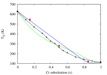
Figure 2: (Color online) Néel temperature as function of the fraction of Cr. Full red circles correspond to the experiments with LuFe_1-xCr_xO₃, and open triangles to MC simulations. The lines correspond to fits of the experiments using Eq.(10) (blue dashed lines) and Eq.(11) (green dot dashed lines), giving $J_{12}=162$ K and $J_{12}=11$ K, respectively. The parameter values of the MC simulation were $J_{22}=436$ K, $J_{11}=79.8$ K, and $J_{12}=106$ K.

From Hashimoto and Dasari expressions very different values of $J_{12}$ are obtained, $11$ K and $162$ K respectively. The value derived from the MC simulations is $J_{12}=106$ K, which is in between the values obtained from Eqs.(11) and(10). Considering that the value of the exchange integral $J_{FeCr}=J_{12}/(2S_{Cr}S_{Fe})$ where $S_{Cr}^{2}=S_{Cr}(S_{Cr}+1)$ and $S_{Fe}^{2}=S_{Fe}(S_{Fe}+1)$ we obtain $J_{FeCr}=28,3$ K, $J_{FeCr}=1.9$ K and $J_{FeCr}=9.25$ K from Eq. (11), Eq. (10) and MC simulations, respectively. The value of $J_{FeCr}$ reported by Dasari et al [Dasari et al., 2012] for YFe_1-xCr_xO₃ ($J_{FeCr}=24.3$ K) is comparably to the value we have found for LuFe_1-xCr_xO₃ using the same equation. The value reported by Kadomtseva et al. for YFe_1-xCr_xO₃ monocrystals using Eq. (11) ($J_{FeCr}=6,64$ K) is considerably lower than the value reported by Dasari et al. in the same compound.

In order to test the mean field approximations, we fitted the MC results with the corresponding expressions (10) and (11). In figure 3 we show a fit of the Néel temperatures obtained from MC simulation using Eq.(10). From this fit we obtained $J_{12}=306$ K which is considerably greater than the value used in MC simulations $J_{12}=106$ K. For comparison we included in Fig. 3 a plot of the mean field expression using the MC simulation value ($J_{12}=106$ K). One can observe that with this value Eq.(10) clearly departs from the results of MC simulations. We concluded that a fit with expression (10) always overestimates the value of the exchange interaction $J_{12}$. Similarly, fitting the MC results using Eq.(11) systematically underestimates $J_{12}$. The accuracy of MF model is expected to be good in low and high Cr content; at intermediate concentrations the effect of the distribution of the interactions is important. Then, a fit which takes into account all the concentration range somehow biases the value of the $J_{12}$ interaction.

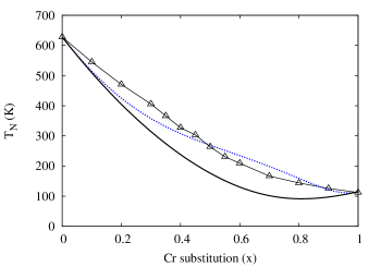
Figure 3: (Color online) Néel temperature as function of the fraction of Cr for LuFe_1-xCr_xO₃. Open triangles correspond to MC simulations and the blue dotted line corresponds to a fit of the MF expression Eq. (10). The parameter that results from the fit is $J_{12}=306$ K. The full line corresponds to a plot of Eq. (10) using the value of MC simulations ($J_{12}=106)$.

In figure 4 we show experimental data for the critical temperature of YFe_1-xCr_xO₃ as a function of the chromium content reported by Dasari et al. Dasari et al. (2012). We also show the data obtained from MC simulations with $J_{FeCr}=9.25$ K tuned to get the best fit with the experimental points. We also include a plot of the mean field expression derived by Dasari et al. Dasari et al. (2012) using the value $J_{FeCr}=24.0$ K which is the value reported by these authors. Finally, a plot of Hashimoto’s expression Hashimoto (1963) Eq.(11) using the value of $J_{FeCr}=6.64$ K reported by Kadomtseva et al Kadomtseva et al. (1977) is also included. In this last work the samples studied were single monocrystals of the YFe_1-xCr_xO₃ compound. MC approach gives a very good agreement with the experiments in all the range of concentrations and the value obtained for $J_{FeCr}=9.25$ K is higher than the reported by Kadomtseva et al. and lower than the reported by Dasari et al. Finally, the values $J_{FeCr}$ obtained from MC for both compounds YFe_1-xCr_xO₃ and LuFe_1-xCr_xO₃ are the same, indicating that the exchange integral is not substantially affected by the substitution of yttrium by lutetium.

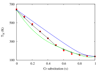
Figure 4: (Color online) Néel temperatures as function of the fraction of Cr for Dasari et al. (2012) YFe_1-xCr_x0₃ (red circles) and MC simulations (open triangles). The blue dashed line corresponds to Eq.(10) using the value of $J_{12}$ reported by Dasari et al [Dasari et al., 2012] and the green dot dashed line corresponds to Eq. (11) using the value of $J_{12}$ reported by Kadomtseva et al [Kadomtseva et al., 1977]

II.2 $T=0$ magnetization

In Fig.5 we show the modulus of the canted magnetization in the z direction ($m_{z}$) at $T=0$ as function of the Cr content which is obtained from MC simulations in a ZFC process. We also plot the modulus of $m_{z}$ obtained using Eq. (6) with the physical constants used in MC simulations. We see a good agreement between MC and the effective model at low and high chromium contents where the model is expected to work better. The local maximum at intermediate concentrations observed in MC simulations is related to a change in the sign of the magnetization. Like in the mean field model at intermediate concentrations the effect of the distributions of the DM bonds is important, and for this reason in this concentration range the effective model departs from MC simulations, in fact the effective model takes into account only averaged values in the distribution of the DM interactions. In addition, the effective canting due to the DM interactions can be approached using the following expression for the magnetization as function of the chromium content

$$m_{z}=\frac{1}{2}[m_{22}P_{1}[x]^{2}+2m_{12}J_{12}^{2}P_{1}[x]P_{2}[x]+m_{22}P_{2}[x]^{2}]$$ (12)

where $m_{ij}$ is the averaged canted magnetization contribution of a pair of spins interacting through the DM interaction. Then, $m_{11}=2\alpha_{11}m_{1}$, $m_{12}=\alpha_{12}(m_{1}+m_{2})$, and $m_{22}=2\alpha_{22}m_{2}$. Here $\alpha_{ij}$ are the average canting angles between ions of type $i$ and $j$ (assuming low angles). According to Eq. (6), $\alpha_{ij}\simeq\frac{D_{ij}}{2J_{ij}}$ for $i=j$, and $\alpha_{12}$ is an effective parameter to be fitted. One can estimate as $\alpha_{12}=\frac{D_{12}}{2J_{21}}$ which turn in $\alpha_{12}=-0.0345$. The fixed parameters are $\alpha_{11}=0.0203$ and $\alpha_{22}=0.0107$ . Fitting Eq. (12) to the MC data we obtain $\alpha_{12}=-0.0258$, showing the consistency of Eq.(12). Moreover, the negative magnetization can be understood from Eq.(12) as an effect of the negative sign of the DM interactions between Fe and Cr ions, which favors the canting of both ions in the negative z direction. Since Fe-Cr pairs are the majority at intermediate values of the Cr concentration $x$, the term in Eq.(12) associated with $m_{12}<0$ is dominant and $m_{z}$ becomes negative.

This local maximum has been reported in experiments carried out in single crystals of the YFe_1-xCr_xO₃ compounds Kadomtseva et al. (1977) where the low temperature magnetization is measured as function of the chromium content.

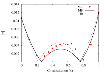
Figure 5: (Color online) Module of the canted magnetization as function of the Cr content at $T=0$ and zero applied magnetic field. Monte Carlo simulations (MC): red circles. Full lines correspond to the effective model Eq. (6) using the same parameters as in the simulation. The dashed lines correspond to a fit using Eq. (12).

II.3 Magnetization reversal

In Fig. 6 we show the $m_{z}$ component of the total magnetization as function of the temperature for $x=0.4$ chromium content obtained by MC simulations using the parameters of the LuFe_1-xCr_xO₃ compound already obtained in section II.1. The cooling is performed under three different applied fields in the $z$ direction; $h=H/J_{22}=5\times 10^{-4},\,1\times 10^{-3}$, and $2\times 10^{-3}$. The arrow indicates the Néel temperature for this composition. We can observe reversal in the magnetization for this composition for the three applied fields. The magnetization increases with the applied field at low temperatures, although the compensation temperature appears to be almost independent of $h$, at least in the small range of values. In this case, $x=0.4$, the compensation temperature is clearly smaller than the Néel temperature. We do not observe magnetization reversal for $x=0.5$ and in fact in the composition range $x>0.4$ the magnetization reversal is unstable. However, the shape of the curve obtained for $x=0.4$ qualitatively reproduces the curves reported in the experiments for yttrium Mao et al. (2011a) (YFe_0.5Cr_0.5O₃) and lutetium Pomiro et al. (2016) (LuFe_0.5Cr_0.5O₃) compounds. Moreover, the ratio between the compensation and Néel temperatures obtained in our simulation $T_{comp}/T_{N}=0.76$ compares well with the experimental valuePomiro et al. (2016) $T_{comp}/T_{N}=0.83$.

Figure 6: Field cooling curves under different applied magnetic fields in the $z$ direction for $x=0.4$. The arrow indicates the ordering temperature obtained from the peak of the susceptibility. The applied field is in units of $J_{22}$ i.e. $h=H/J_{22}$.

In Fig. 7 we show FC magnetization curves with $h=2\times 10^{-3}$ for $x=0.4$, and curves obtained through a mean field approach. Here we have measured in MC simulations separately the temperature dependence of the total magnetization of the Fe³⁺ ions and that of the Cr³⁺ ions. We can see that below the Néel temperature the magnetization due to the Fe³⁺ ions aligns in the direction of the magnetic field, while the magnetization due to the Cr³⁺ ions is opposite to the field. In this way, when the field breaks the inversion symmetry along the $z$ axis the Zeeman energy is reduced due to the coupling of the larger magnetic moments of the Fe³⁺ ions. The different temperatures dependencies in the magnetization of Fe³⁺ and Cr³⁺ ions turns into the magnetization reversal. For lower compositions ($x\leq 0.3$) the Fe³⁺ ions are also aligned in the direction of the applied field but magnetization reversal is not observed because the contribution to the magnetization of Fe³⁺ is dominant.

In this figure we also show mean field curves which are obtained through Eq. (4) using a molecular field approximation for the dependence of the sublattice magnetization on the temperature. This approximation agrees very well with MC results for the sublattice magnetization. In the calculation of the mean field curves showed in Fig. Fig. 7 we used the same parameters than in MC results. These curves reproduce the features observed in MC results. However, in this case the compensation temperature (see inset) is much closer to the Néel temperature. From an analysis of the different energy term contributions, Eq. (4), we observed that close to the Néel temperature the Zeeman term is the most important hence the coupling with the field at high temperatures rules the magnetization process and induces the symmetry breaking. In the lower temperature range DM interactions prevail and convey the reversal of the magnetization.

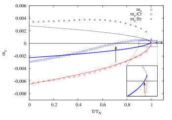
Figure 7: (Color online) Field cooling curves with an applied fields in the $z$ direction for $x=0.4$. The applied field ($h=0.002$) is the same for all the curves. The symbols with lines correspond to MC simulations and lines to MF results. MC simulations: chromium magnetization (black triangles), iron magnetization (red circles) and total magnetization (blue squares). MF calculations: chromium magnetization (black dotted line), iron magnetization (red dashed line) and total magnetization (blue continuous line). The arrows indicate the compensation temperatures in both cases, and the inset is a zoom of MF curves close to the ordering temperature.

III Discussion

Monte Carlo simulations using the proposed microscopic classical model reproduce the whole phenomenology of both LuFe_1-xCr_xO₃ and YFe_1-xCr_xO₃ compounds as the chromium content is varied. From these simulations it turns out that the superexchange interaction between Cr³⁺ and Fe³⁺ ions is lower than the super-exchange interaction between Fe³⁺ and Fe³⁺, and greater than the super-exchange between Cr³⁺ and Fe³⁺ ions i.e. $J_{22}>J_{12}>J_{11}$. From the fit of our experimental results with different mean field expressions, Eqs. (10) and (11) we obtained $J_{12}=162$ K and $J_{12}=11$ K, respectively.

These results show a big dispersion depending of the expression used to fit the experiments. In particular, the value obtained from MC simulations, $J_{12}=106$ K, is in between this two values. The values of $J_{12}$ available in the literature for Y perovskites YFe_1-xCr_xO₃, also show an important dispersion. For instance, $J_{12}=139$ K, when Eq. (10) is used in polycrystals Dasari et al. (2012) and $J_{12}=38$ K has been reported in single crystals Kadomtseva et al. (1977) using Eq. (11). Such large sensitivity to the details of the particular mean field approximation is not surprising in a solid solution, where the interplay between thermal fluctuations and the inherent disorder of the solution is expected to be very relevant to determine thermal properties. Consistently, the experimental results are better described by the MC simulations than by the MF expressions. Hence, we expect our estimation of $J_{12}$ to be more reliable than the previous ones. In addition, our results suggest that the exchange constant (and therefore the general behavior) is not substantially affected by the substitution of yttrium by lutecium.

The zero temperature magnetization obtained from MC simulations in a ZFC process, which is due to the canting of the AFM spins in the $z$ directions, is well approached by an effective coarse grain model in the range of low and high chromium contents as expected. A bump in the magnetization is observed in MC simulations at intermediate concentrations which is a signature of the magnetization reversal. This bump is also observed in the coarse grain approach but is less pronounced. The difference between MC simulations and the effective model at intermediate concentrations is expected since the coarse grain approach does not take into account information on the distribution of the ions in the lattice which is important at intermediate Cr concentrations.

Magnetization reversal is observed at intermediate chromium contents $x=0.4$ in a ZFC process depending on the value of $D_{12}(\simeq 1.7\times 10^{-2}J_{22})$. When the field is increased above a certain threshold MR disappear, and the magnetization points in the direction of the applied field in whole temperature range. The presence of magnetization reversal is very sensitive to the value of the DM interaction between Cr³⁺ and Fe³⁺ ions and also to the value of superexchange $J_{12}$ interaction. We do not observe magnetization reversal in MC simulations at $x=0.5$ such as is observed in experiments. This could be due to size effects which are particularly important in systems that includes disorder. In fact, the fields we used to obtain the ZFC curves (e.g. $h=0.001$ correspond to $B\simeq 0.13$ T) are much greater that the ones used in experiments (e.g. $B\sim 0.01$ T). A reduction of the fields in MC is only possible in larger systems.

Summarizing, Monte Carlo simulations based in a Heisenberg microscopic classical model reproduce the critical temperatures observed in experiments. Besides this is a classical model, MC fit can provide a better estimation of $J_{12}$ since in this model the random occupation of the Cr³⁺ and Fe³⁺ ions is taken into account. Regarding the phenomena of magnetization reversal, we found it for appropriated values of the superexchange and the Dzyaloshinskii-Moriya interactions at intermediate Cr concentrations. However, the mechanism for the appearance is subtle and further investigations are needed to shed light on this point.