ZNNi – Maximizing the Inference Throughput of 3D Convolutional Networks on Multi-Core CPUs and GPUs

Abstract

Sliding window convolutional networks (ConvNets) have become a popular approach to computer vision problems such as image segmentation, and object detection and localization. Here we consider the problem of inference, the application of a previously trained ConvNet, with emphasis on 3D images. Our goal is to maximize throughput, defined as average number of output voxels computed per unit time. Other things being equal, processing a larger image tends to increase throughput, because fractionally less computation is wasted on the borders of the image. It follows that an apparently slower algorithm may end up having higher throughput if it can process a larger image within the constraint of the available RAM. We introduce novel CPU and GPU primitives for convolutional and pooling layers, which are designed to minimize memory overhead. The primitives include convolution based on highly efficient pruned FFTs. Our theoretical analyses and empirical tests reveal a number of interesting findings. For some ConvNet architectures, cuDNN is outperformed by our FFT-based GPU primitives, and these in turn can be outperformed by our CPU primitives. The CPU manages to achieve higher throughput because of its fast access to more RAM. A novel primitive in which the GPU accesses host RAM can significantly increase GPU throughput. Finally, a CPU-GPU algorithm achieves the greatest throughput of all, $10\times$ or more than other publicly available implementations of sliding window 3D ConvNets. All of our code has been made available as open source project.

I Introduction

Waving the banner of “deep learning,” researchers have revived the use of convolutional networks (ConvNets) for computer vision. The revival has been driven by increases in the speed of ConvNet training made possible by GPU implementations [1, 2, 3, 4]. Here we are concerned with the problem of inference, applying a previously trained ConvNet to a new image. Fast inference is critical for big data applications involving large numbers of images and/or very large images. Billions of photos and millions of videos are shared online every day [5, 6]. Scientists are also generating large amounts of image data. For example, high-speed electron microscopy can generate a petascale 3D image from a cubic millimeter of brain in a few weeks [7]. We will focus on 3D ConvNets, which are relevant for both videos and 3D images. 2D ConvNets are regarded as a special case that is less computationally costly.

In contemporary computer vision, researchers are most familiar with applying ConvNets to image-to-label transformations. For example, in object recognition the input is an image of an object and the desired output is the class of the object. However, ConvNets can also be used for image-to-image transformations. In this context, a ConvNet acts like a more complex version of a typical filtering operation in image processing. The ConvNet is applied to a window that slides over the input image. For each location of the window, the ConvNet outputs a set of numbers, effectively producing a set of output images, each with the same resolution as the input image.

For speeding up sliding window inference, a seemingly trivial detail about image borders turns out to be a bottleneck. Inference is less efficient near the borders, and this inefficiency is proportionally smaller for a larger input image. So efforts to maximize throughput tend to bump into the constraint of limited RAM. (This is not the case for ConvNet training, where there is typically some range of input sizes that is optimal for training speed.) An apparently slower algorithm may end up having higher throughput if it can process a larger image within the constraint of the available RAM.

Figure 1: Diagram of all layers primitives. The red primitives are wrappers primitives provided by CuDNN. The green primitives are the novel primitives introduced in this paper.

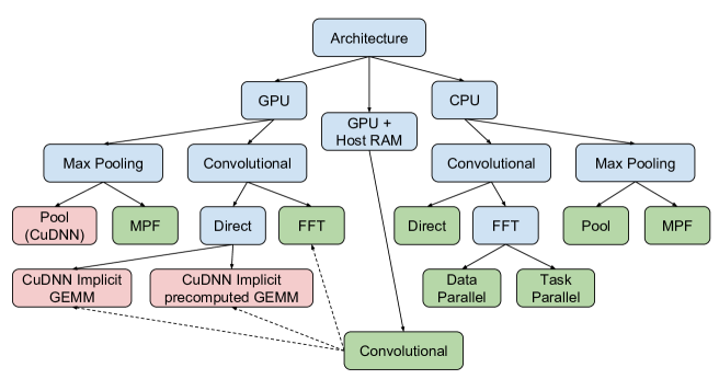
We consider ConvNet architectures that contain both convolutional and pooling layers. GPU implementations such as cuDNN provide a number of primitives for both kinds of layers. A particular architecture is implemented by combining primitives. In line with this approach, we introduce a number of new layer primitives for the CPU and GPU (Fig. 1). These are designed to have low memory overhead, which should be important for high throughput as mentioned above.

Our new convolutional primitives are either direct or FFT-based. For the latter, we introduce new implementations of pruned FFTs that are faster (for kernels on average $5\times$ for CPU and $10\times$ for GPU) while using less memory. Our FFT-based convolutional primitive for the GPU is designed to use much less memory than the algorithm proposed by [8, 9] and implemented in fbfft. We provide two new FFT-based convolutional primitives for the CPU. The task parallel version is more efficient if the number of input images and the number of output images are both large, but at the cost of more memory overhead than the data parallel version. The task parallel algorithm is designed to use less memory than the one previously proposed for ConvNet training [10]. To evaluate our novel primitives, we include comparisons with the direct convolutional primitives in cuDNN. We also provide a new direct convolutional primitive for the CPU, but this turns out to be less useful than our FFT-based primitives in most circumstances.

In empirical tests, we combine the primitives to maximize throughput for CPU-only and GPU-only algorithms. In some cases, our FFT-based GPU primitives outperform the cuDNN primitives by a large margin. The CPU-only algorithm may achieve higher throughput than the GPU-only algorithm because the CPU has fast access to more RAM, even if it is capable of fewer floating point operations (FLOPs) per second.

To work around the limited onboard RAM of the GPU, we introduce a novel GPU + host RAM primitive. We show that using this new primitive can lead to much higher throughput, in spite of the slower communication speed between GPU and host RAM.

Finally, we study a CPU-GPU algorithm, in which the first layers of the ConvNet are computed by the CPU and the later layers are computed by the GPU. The algorithm is pipelined to utilize the CPU and GPU efficiently. This yields the highest throughput of all the algorithms, sometimes even greater than the sum of throughputs of GPU + host RAM and CPU-only.

We also compare with other 3D sliding window max-pooling ConvNet implementations. To the best of our knowledge, the only publicly available ones are the Caffe implementation of [11], ZNN [10], and ELEKTRONN [12]. (The last is the only competitor that is specifically optimized for inference.) For comparison, we also include a baseline implementation that utilizes the simple pooling primitives of cuDNN to perform the naive algorithm of computing all subsamplings of the output. For four representative ConvNet architectures running on a Titan X and/or a 4-way Intel Xeon E7 8890v3 machine with 256 GB RAM, our CPU-only, GPU-only, GPU + host RAM, and CPU-GPU implementations outperform all competitors. In particular, our CPU-GPU implementation wins by a factor of roughly $10\times$ or more in all cases.

We focus on throughput (number of output voxels per unit time) as the performance metric. A related metric is energy consumed per voxel. For a given CPU or GPU, maximizing throughput is equivalent to minimizing energy consumption, assuming that the power consumption is roughly constant in time. An interesting implication of our work is that in some situations the most economical way of increasing inference throughput may be to increase host RAM rather adding more GPUs or CPUs.

II Throughput of sliding window inference

Sliding window ConvNets were originally applied to detect and/or localize objects in a larger image [13], and this usage has been revived [14]. Here each output image represents the probability that an object of a certain class is located at a voxel. Sliding window ConvNets have also been applied to image segmentation, to produce an output image representing the probability that a voxel is a boundary between objects or not [15]. And they have been applied to semantic segmentation, the problem of labeling each voxel in an input image by the class of the object to which it belongs [16]. In general, sliding window ConvNets are increasing in popularity as they are applied to more and more problems in computer vision. However, transforming image-to-image is even more computationally costly than image-to-label, so the need for speeding up sliding window ConvNets is especially acute.

In large scale sliding window inference, the input image is divided into smaller input patches. These are transformed by the ConvNet into output patches, which are recombined to generate the output image. This divide-and-conquer approach is motivated by both time and space considerations. The computation can be sped up by assigning the patches to multiple workers. Also if the computation were not divided, it might not fit in the RAM available to a single worker.

Each output patch is smaller than the input patch, because the sliding window is restricted to be entirely contained within the input image. (This is analogous to a “valid” convolution in MATLAB.) Therefore the input patches are chosen to overlap so that the output patches exactly cover the output image without overlap. (This is analogous to the overlap-save or overlap-scrap method for computing a single convolution described in signal processing textbooks.)

We define the throughput of a single worker as the number of voxels in the output patch divided by the time required for the worker to process a single patch. In this paper, a worker will be a single shared-memory machine, either CPU or GPU or combination of the two. Our goal is to maximize worker throughput.

When computing ConvNet outputs for nearby locations of the sliding window, some of the arithmetic operations are identical. For efficiency it is important to reuse the results of these operations. For ConvNets with convolutional layers only, this happens naturally as the output patch is the same resolution as the input patch. If there are pooling layers, however, the output patch produced by a ConvNet is a subsampling of the output of a sliding window ConvNet. To obtain the entire output image, one must compute all subsamplings with different offsets separately, and then combine them. This algorithm does not efficiently reuse computations for nearby output voxels.

Here we instead provide pooling primitives that compute max-pooling fragments (MPF), a more efficient strategy for sliding window computations [17, 18]. ELEKTRONN is the only other publicly available package with MPF support known to us (http://elektronn.org). The MPF algorithm computes the same results as the approach known as “dilated convolution”[19], “strided kernels”[11], “max filtering”[10], or “filter rarefaction”[20].

While MPF does efficiently reuse computation within a patch, the division into patches does itself incur a cost. Reuse cannot happen for nearby locations in different output patches, assuming the computations on the patches are done independently. For example, it is highly inefficient to make the input patch the same size as the sliding window, which results in no reuse at all across different locations of the sliding window. It is more efficient to increase the size of the input patch, to reduce the fraction of voxels near the border and thereby reduce inefficiency due to lack of reuse.

Consequently memory overhead becomes important, if the goal is to maximize throughput. An apparently faster algorithm may end up with inferior throughput if it cannot process a large input patch using the available RAM. Later on, we will introduce a set of novel primitives for computing the layers of a ConvNet, which are designed to have low memory overhead as well as to be fast. The primitives include convolutional and max-pooling layers. (Our approach also can be extended to other kinds of pooling layers.) As a prelude to the layer primitives, we first introduce lower-level FFT primitives which turn out to be important for efficient convolution.

III Pruned FFT

Improving the efficiency of convolution is crucial, because this computation is performed so many times in a ConvNet. The advantages of FFT convolution have been shown for 2D ConvNets running on GPUs [8, 9], and 3D ConvNets running on CPUs [10].

In FFT convolution the kernel and the image are zero-padded to a common size. Since the kernel is typically much smaller than the image, the padded kernel consists mostly of zeros. Ignoring the zeros is known as FFT pruning, and can provide speedup. We propose and implement such an algorithm, for both the CPU and GPU. Our approach achieves an average of $5\times$ speedup over the naive approach on the CPU and $10\times$ speedup on the GPU.

The speedup is expected to be large for a ConvNet, which typically contains many more kernel FFTs than image FFTs. The speedup is more modest for a single convolution, which requires one padded kernel FFT, one image FFT, and one inverse FFT.

While our pruned FFT algorithms give a substantial speedup, understanding them is not necessary for understanding the rest of our contributions. The reader may prefer to skip to the next section on how pruned FFTs are used to compute the convolutional layers.

Figure 2: Pruned FFTs. The dark blue voxels show the locations of the nonzero elements of the image after zero-padding.

III-A General algorithm

For 3D FFT-based convolution, the 3D images $x$ and $y$ are first zero-padded to the same size. The inverse FFT of the point-wise product contains the result of the convolution. The images $x$ and $y$ can be zero-padded to any size, as long as their size is equal.

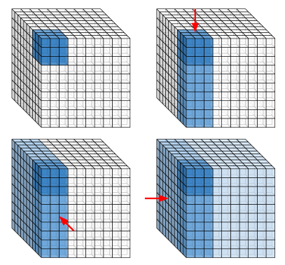
A 3D FFT is obtained by computing 1D FFTs along the three dimensions. Some of these 1D FFTs are of an array with all elements equal to $0$. These are unnecessary to compute as the FFT of an all zeros signal is all zeros.

We can reduce the amount of computation by computing only necessary 1D transforms. When computing the FFT of a trainable kernel of size $k^{3}$ zero padded to size of $n^{3}$, instead of naively computing $n^{2}$ 1D FFTs along each dimension, which takes $Cn^{3}\log n^{3}$ we could first only do $k^{2}$ FFTs along one dimension, then $k\times x$ along then next, and finally $n^{2}$ along the last dimension, as shown on Fig. 2. This approach reduces the computational cost from $Cn^{3}\log n^{3}$ to $Cn\log n[k^{2}+k\cdot n+n^{2}]$. As most of the FFTs are performed on kernels, and as the kernel sizes are usually much smaller compared to the image sizes ($k\ll n$), we could reduce the computation cost by nearly two thirds.

III-B CPU implementation

Suppose we would like to compute the FFT of an $x\times y\times z$ image zero-padded to an $x^{\prime}\times y^{\prime}\times z^{\prime}$ image.

The $x\times y\times z$ image is zero-padded to $x^{\prime}\times y\times z$. This is easily implemented by doing a linear copy of the memory, and zero-padding the rest. We then perform $y\cdot z$ 1D real to complex FFT transforms along the $x$ direction. The FFTs are performed out of place into a pre-allocated, and zero-initialized complex-valued $\lfloor\frac{x^{\prime}}{2}\rfloor+1\times y^{\prime}\times z^{\prime}$ image. We then perform in-place 1D transforms along the $y$ direction, followed by the $z$ direction.

The inverse FFT is computed by following the above steps in reverse order. The 1D FFTs can either be done serially, or by $N$ workers in parallel (in a parallel for loop).

This method induces a memory overhead of $x^{\prime}\times y\times z$, a space required for zero–padding the image along $x$ direction in the first step of the algorithm.

III-C GPU implementation

On the GPU, we always perform FFTs on $b$ 3D images simultaneously, in order to achieve high utilization of the many GPU threads.

A set of $b$ 3D images can be represented as a 4D tensor. We need to perform 1D FFTs along the three least significant dimensions. Our algorithm computes the 3D FFTs as a series of tensor transforms  and 1D FFTs along the least significant dimension of the tensor.

When computing the FFT transforms of $b$ 3D images each of size $x\times y\times z$ padded to $x^{\prime}\times y^{\prime}\times z^{\prime}$, the size of the 4D input tensor $I$ is $b\times x\times y\times z$. First, 1D in–place real to complex 1D transforms along the $z$ direction are performed. We prepare the input by extending the 4D tensor along the $z$ direction to fit the result. The transform will need to contain $z^{\prime\prime}=z^{\prime}/2+1$ complex numbers, and we need twice as many reals. A 4D tensor $I^{1}$ of size $b\times x\times y\times 2z^{\prime\prime})$ is first initialized to zero, and appropriate elements from the input are filled in (elements $I_{i,j,k,l}$ get mapped to $I^{1}_{i,j,k,l}$ while the rest of elements of $I^{1}$ are set to zero).

A batch of $b$ in–place real to complex 1D transforms are then performed. The result represents a 4D complex tensor $\widetilde{I}^{1}$ of size $b\times x\times y\times z^{\prime\prime}$. Note that all the 1D transforms are done on contiguous memory chunks (along the least significant dimension).

In the next step we perform in-place complex to complex transforms along the $y$ direction. To do this the elements of $\widetilde{I}^{1}$ are permuted into another 4D tensor $\widetilde{I}^{2}$ of size $b\times x\times z^{\prime\prime}\times y^{\prime}$, such that the element $\widetilde{I}^{1}_{i,j,k,l}$ gets mapped to $\widetilde{I}^{2}_{i,j,l,k}$ and the rest of $\widetilde{I}^{2}$ is zero–filled. We then perform in-place complex to complex transforms along the least significant dimension of $\widetilde{I}^{2}$.

In the final step, we perform the transform along the $x$ direction. We permute $\widetilde{I}^{2}$ into a new 4D complex tensor $\widetilde{I}^{3}$ of size $b\times z^{\prime\prime}\times y^{\prime}\times x^{\prime}$. An element $\widetilde{I}^{2}_{i,j,k,l}$ is mapped to $\widetilde{I}^{3}_{i,k,l,j}$. Complex to complex in-place transforms are performed along the least significant dimension of $\widetilde{I}^{3}$.

As we only perform point-wise multiplications of transformed images, or take the inverse transforms of them, we can just keep the result in this representation – not waste computation doing extra permuting.

The inverse transform can be performed taking the same steps in reverse order.

III-D Implementation details

Our approach uses $3$rd party libraries to perform each batch of 1D FFTs. Depending on the library implementation, the size to which we pad the 3D image can greatly influence the computational complexity.

On the CPU we use either fftw or Intel MKL, and pad the images (and kernels) to sizes that can be written in the form of $2^{a}3^{b}5^{c}7^{d}11^{e}13^{f}$. When Intel MKL is used any such size is allowed, however, when fftw is used we only allow sizes for which $e+f$ is either $0$ or $1$ [21, 22]. On the GPU we use cuFFT [23], which has optimized algorithms only for sizes of the form $2^{a}3^{b}5^{c}7^{d}$.

4D tensor permuting requires a lot of indexing calculation, which can involve a lot expensive division and modulus operations. Sometimes these operations are more expensive than the actual 1D FFT transforms performed. We improve the performances by only using multiplications by a pre–computed magic numbers and shift operations as described in  [24]. Image reshaping is easily implemented using the Thrust CUDA library [25].

We limit the large cuFFT memory overhead for computing batches of 1D transforms by splitting the batch computation into sub–batches of 1D transforms. We make sure that the sub–batch size is still large enough to utilize all the computational power, but limit the size so that we limit the memory overhead.

The memory overhead of the algorithm is due to the fact that we do out-of-place permuting of the 4D tensor, and requires space for $b\cdot x\cdot y^{\prime}\cdot z^{\prime\prime}$ complex numbers. This, however, will not increase the memory overhead of our algorithm for convolutional layers on the GPU, as it already needs a temporary tensor of size $b\cdot x^{\prime}\cdot y^{\prime}\cdot z^{\prime\prime}$ for other purposes, which we can use as the scratch space for computing the FFT transforms.

Additional, relatively small, overhead comes from the memory required by cuFFT to perform a batch of 1D transforms. By dividing the batch into sub–batches we essentially limit this overhead to a pre–defined constant amount of memory.

IV Convolutional layers

We begin with the primitives for the convolutional layers, which are the most computationally intensive.

The input to a convolutional layer is a tuple of $f$ images, and the output a tuple of $f^{\prime}$ images. We want to process a batch of $S$ inputs to yield a batch of $S$ outputs, via

$$O_{s,j}=\sum_{i=1}^{f}w_{ji}\ast I_{s,i}$$

for $1\leq s\leq S$ and $1\leq j\leq f^{\prime}$. Here $I_{s,i}$ is the $i^{th}$ image of the $s^{th}$ input in the batch, and $O_{s,j}$ is the $j^{th}$ image of the $s^{th}$ output in the batch, and $w_{ji}$ is the kernel from the $i^{th}$ image in an input tuple to the $j^{th}$ image in an output tuple.

We will assume 3D images and kernels. If $I_{s,i}$ has size $\vec{n}=\langle n_{x},n_{y},n_{z}\rangle$ and $w_{ji}$ has size $\vec{k}=\langle k_{x},k_{y},k_{z}\rangle$, then we can regard $I$ as a 5D tensor of size $S\times f\times n_{x}\times n_{y}\times n_{z}$, $w$ as a 5D tensor of size $f^{\prime}\times f\times k_{x}\times k_{y}\times k_{z}$, and $O$ as a 5D tensor of size $S\times f^{\prime}\times n_{x}^{\prime}\times n_{y}^{\prime}\times n_{z}^{\prime}$, where $\vec{n}^{\prime}=\vec{n}-\vec{k}+\vec{1}$.

We will refer to the sizes of the 5D tensors $I$ and $O$ as input and output shape, respectively. The relationship between input shape and output shape depends on kernel size as in Table I.

Layer	Input shape	Output shape	FLOPS
Convolutional – Direct	$S\times f\times n^{3}$	$S\times f^{\prime}\times[n-k]^{3}$	$S\cdot f^{\prime}\cdot f\cdot n^{3}\cdot k^{3}$
Convolutional – FFT–based	$S\times f\times n^{3}$	$S\times f^{\prime}\times[n-k]^{3}$	$S\cdot 3Cn^{3}\log n[f^{\prime}+f]+4Sf^{\prime}\cdot f\cdot n^{3}+f\cdot f^{\prime}\cdot Cn\log n[k^{2}+k\cdot n+n^{2}]$
Max Pooling	$S\times f\times n^{3}$	$S\times f\times[n/p]^{3}$	$S\cdot f\cdot n^{3}$
Max Fragment Pooling	$S\times f\times n^{3}$	$[S\cdot p^{3}]\times f\times(n/p)^{3}$	$S\cdot f\cdot n^{3}\cdot p^{3}$

TABLE I: Relation between input and output shapes for convolutional and pooling layers, along with computational complexities. Input shape is for a batch of $S$ inputs, each of which is an $f$-tuple of 3D images with size $n^{3}$, and output shape is analogous. The 3D kernel has size $k^{3}$. The pooling window has size $p^{3}$, and the constant $C$ for the FFT complexity depends on the FFT implementation.

IV-A CPU algorithms

We propose three parallel algorithms for the convolutional layer that are suited for multi-core CPUs. The first algorithm performs direct convolution, whereas the other two use FFT based convolutions.

IV-A1 Direct convolution algorithm

• $\textnormal{Convolutional-Forward-FFT-CPU1}(I,w,S,f,f^{\prime},\vec{n},\vec{k})$
     1$\vec{n}^{\prime}=\vec{n}-\vec{k}+\vec{1}$ 2$O\mathrel{\hskip 1.0pt=\hskip 1.0pt}\textnormal{5D-Real-Tensor}(S,f^{\prime},n^{\prime}_{x},n^{\prime}_{y},n^{\prime}_{z})$ 3parallel for $i\mathrel{\hskip 1.0pt=\hskip 1.0pt}0\ \textrm{{to}}\ S-1$ 4 parallel for $j\mathrel{\hskip 1.0pt=\hskip 1.0pt}0\ \textrm{{to}}\ f^{\prime}-1$ 5 for $k\mathrel{\hskip 1.0pt=\hskip 1.0pt}0\ \textrm{{to}}\ f-1$ 6 $O_{i,j}\mathrel{\hskip 1.0pt=\hskip 1.0pt}O_{i,j}+\textnormal{Convolve}(I_{i,k},w_{j,k})$ 7$\textnormal{Free-Memory}(I)$ 8return $O$

Algorithm 1 Multi-core algorithm for a convolutional layer using direct convolution.

The computation is parallelized by two parallel for loops such that each image of each output in the batch is computed in parallel on a different working thread (see Algorithm 1). The parallel for loops are implemented using Intel thread building blocks such that the work is evenly divided over the available cores.

We provide one implementation using naive convolution and the other using Intel MKL. The latter is $2\times$ faster on average, but requires extra memory for a temporary image where a result of convolution is stored before accumulating it to the output image. The memory overhead of both implementations is given in Table II.

CPU algorithm	Memory required
Direct (naive)	$S\cdot f\cdot n+S\cdot f^{\prime}\cdot n^{\prime}$
Direct (MKL)	$S\cdot f\cdot n+S\cdot f^{\prime}\cdot n^{\prime}+T\cdot n^{\prime}$
FFT algorithm 1	$\max\begin{cases}S\cdot f\cdot(n+\widetilde{n})\\ S\cdot f^{\prime}\cdot n^{\prime}+(S\cdot f+1)\cdot\widetilde{n}\end{cases}$
FFT algorithm 2	$\max\begin{cases}S\cdot f\cdot(n+\widetilde{n})\\ S\cdot(f+f^{\prime})\cdot\widetilde{n}+T\cdot\widetilde{n}\\ S\cdot f^{\prime}\cdot(n^{\prime}+\widetilde{n})\end{cases}$
GPU algorithm	Memory required
cuDNN (default)	$S\cdot f\cdot n+S\cdot f^{\prime}\cdot n^{\prime}$
cuDNN (precomp)	$2S\cdot f\cdot n+S\cdot f^{\prime}\cdot n^{\prime}$
FFT	$K+\max\begin{cases}S\cdot f\cdot(n+\widetilde{n})+f\cdot\widetilde{n}\\ S\cdot(f+f^{\prime})\cdot\widetilde{n}+2f\cdot\widetilde{n}\\ S\cdot f^{\prime}\cdot(n^{\prime}+\widetilde{n})+f^{\prime}\cdot\widetilde{n}\end{cases}$

TABLE II: Memory required by different implementations. $S$ is the batch size, $f$ and $f^{\prime}$ represent the number of input/output images of the layer. $n$ and $n^{\prime}$ represent the number of pixels in each input/output image, and $\widetilde{n}$ represents the number of elements in the transformed image. $K$ is pre–defined constant amount of memory allocated for cuFFT, and $T$ is the number of available cores for the CPU algorithms.

IV-A2 Data parallel FFT-based algorithm

The computationally intensive operations are individually parallelized (see Algorithm 2). More specifically each FFT and inverse FFT transform is done in parallel as explained in the previous section. The Parallel-MAD function computes a series of multiply-add operations of complex numbers in parallel by dividing the range into roughly equal sub-ranges, each of which is executed on a single core.

• $\textnormal{Convolutional-Forward-FFT-CPU1}(I,w,S,f,f^{\prime},\vec{n},\vec{k})$
       1$\vec{n}^{\prime}=\vec{n}-\vec{k}+\vec{1}$ 2$\vec{\widetilde{n}}=\textnormal{FFT-Optimal-Size}(\vec{n})$ 3$\widetilde{I}\mathrel{\hskip 1.0pt=\hskip 1.0pt}\textnormal{5D-Complex-Tensor}(S,f,\lfloor\widetilde{n}_{x}/2\rfloor+1,\widetilde{n}_{y},\widetilde{n}_{z})$ 4for $i\mathrel{\hskip 1.0pt=\hskip 1.0pt}0\ \textrm{{to}}\ S-1$ 5 for $j\mathrel{\hskip 1.0pt=\hskip 1.0pt}0\ \textrm{{to}}\ f-1$ 6 $\widetilde{I}_{i,j}\mathrel{\hskip 1.0pt=\hskip 1.0pt}\textnormal{Parallel-FFT}(I_{i,j})$ 7$\textnormal{Free-Memory}(I)$ 8$O\mathrel{\hskip 1.0pt=\hskip 1.0pt}\textnormal{5D-Real-Tensor}(S,f^{\prime},n^{\prime}_{x},n^{\prime}_{y},n^{\prime}_{z})$ 9$\widetilde{O}\mathrel{\hskip 1.0pt=\hskip 1.0pt}\textnormal{4D-Complex-Tensor}(S,\lfloor\widetilde{n}_{x}/2\rfloor+1,\widetilde{n}_{y},\widetilde{n}_{z})$ 10$\widetilde{w}\mathrel{\hskip 1.0pt=\hskip 1.0pt}\textnormal{3D-Complex-Tensor}(\lfloor\widetilde{n}_{x}/2\rfloor+1,\widetilde{n}_{y},\widetilde{n}_{z})$ 11for $i\mathrel{\hskip 1.0pt=\hskip 1.0pt}0\ \textrm{{to}}\ f^{\prime}-1$ 12 for $j\mathrel{\hskip 1.0pt=\hskip 1.0pt}0\ \textrm{{to}}\ f-1$ 13 $\widetilde{w}=\textnormal{Parallel-FFT}(w_{i,j})$ 14 for $k\mathrel{\hskip 1.0pt=\hskip 1.0pt}0\ \textrm{{to}}\ S-1$ 15 $\textnormal{Parallel-MAD}(\widetilde{I}_{k,j},\widetilde{w},\widetilde{O}_{k})$ 16 for $k\mathrel{\hskip 1.0pt=\hskip 1.0pt}0\ \textrm{{to}}\ S-1$ 17 $O_{k,i}\mathrel{\hskip 1.0pt=\hskip 1.0pt}\textnormal{Parallel-Inverse-FFT}(\widetilde{O}_{k})$ 18$\textnormal{Free-Memory}(\widetilde{I})$ 19$\textnormal{Free-Memory}(\widetilde{O})$ 20$\textnormal{Free-Memory}(\widetilde{w})$ 21return $O$

Algorithm 2 Multi-core algorithm for a convolutional layer

The memory requirement of the algorithm equals to the maximal amount of memory required by the algorithm at any single point of time during the execution, and is given in Table II.

IV-A3 Task parallel FFT-based algorithm

The main quantities of the task parallel algorithm are: (1) breaking up the computation required by the convolutional layer into tasks that operate on independent chunks of memory, (2) creating a task dependency graph, and (3) scheduling the tasks for execution.

There are five different task types:

• Input image transform task computes the forward FFT transform of a single input image.

• Kernel transform task computes the forward FFT transform of a single kernel.

• Multiply-add task computes the point-wise product of an input image and a kernel FFT accumulating the result to an appropriate image transform.

• Output image transform task computes the inverse FFT of the appropriate accumulated image transform. This task is also responsible for adding the bias and applying the transfer function.

• Synchronization tasks, beside serving as synchronization points are the only tasks responsible (and only ones allowed) to allocate and/or deallocate memory.

Figure 3: Task dependency diagram of a task–based convolutional layer.

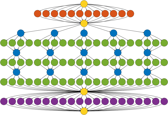
The task dependency graph of all the tasks required for computing the output images of a convolutional layer with four input and five output images for a batch size of four is shown on Fig. 3. The tasks are created and queued when all their dependencies have been satisfied. There are four synchronization tasks effectively dividing the computation into three stages. The layout of the kernel transform tasks forms a grid, with the number of columns equal to the number of output images, and the number of rows equal to the number of input images. The task of the $i^{th}$ column and $j^{th}$ row computes the transform of the kernel $w_{i,j}$. Furthermore, each such task has $S$ dependent multiply-add tasks, where $S$ is the batch size of the input (equal to four in Fig. 3). The $k^{th}$ dependent multiply-add task of a kernel transform task in column $i$ and row $j$ accumulates the product of the transforms of the $j^{th}$ input image of the $k^{th}$ batch and the filter $w_{i,j}$ to the transform of the $i^{th}$ output image of the $k^{th}$ batch.

The tasks are executed by $N$ worker threads, where $N$ equals the number of available cores (or virtual cores, when hyper–threading is enabled). Each worker thread is pinned to a single core. This means that there is 1–1 relation between the workers and the available cores – each worker is allowed to run only on a specific hardware core, as described in [26]. For this reason, we will use “worker thread” and “core” interchangeably.

The first synchronization task allocates memory for the FFT transforms of the input images. The number of dependent input image transform tasks equals the number of input images times the batch size $S$. They are then executed by the $N$ worker threads, such that each worker picks up an arbitrary task and executes it.

The last thread to complete the execution of an input image transform task immediately executes the second synchronization task. This tasks deallocates the memory holding the input images, as their values are no longer required. It then allocates memory for the transforms of the output images. At this point $M$ threads are chosen as primary threads, where $M$ is the maximum of $N$ – total number of threads, and the number of output images. The primary threads are chosen so that they are evenly distributed over multiple physical chips. Each primary thread is given a temporary buffer equal to the size required to fit the transform of a padded kernel for that layer.

The kernel transform tasks and multiply-add tasks are then scheduled for execution based on their distance to the sink node of the task dependency graph, such that the more distant nodes get scheduled first. The scheduling has two additional constraints: (1) the kernel transform tasks can only be executed by a primary thread, and (2) its dependent multiply-add tasks can only be executed by worker threads that are pinned to the cores on the same physical chip.

This strategy is chosen over the popular alternative approach to task scheduling based on work stealing [27, 28] because it divides the work more evenly over multi–chip machines and further increase cache locality. On a 4-way machine it yields more deterministic results – very little variance in run-time and average of 20% speed improvement over the alternative.

The last multiply-add task to complete executes the third synchronization task. This task deallocates the memory buffers given to the primary threads as well as the memory used to store the transforms of the input images. It also allocates the memory to store the final result – the output images.

The number of output image transform tasks equals the number of output images times the batch size. The tasks are executed by all $N$ workers, such that each worker picks up an arbitrary task and executes it. The last output image transform task to finish also executes the final synchronization task, which frees the memory required for the output image transforms.

The task parallel algorithm requires that both $f\cdot S$ and $f^{\prime}\cdot S$ be large enough (at least the same size as the number of available cores) in order to efficiently utilize all the cores. In such cases they can be much more efficient than the data parallel algorithm, as the tasks operate on independent data (thus reducing false–sharing ). It further improves the performances on multi–chip systems, by minimizing the data sharing between cores on different chips. On a 4–way Intel Xeon E7–8890 v3 machine the task parallel algorithm is $10\times$ faster than the data parallel one (for large enough $f^{\prime}\cdot S$ and $f\cdot S$).

As shown later, this is the implementation that is optimal in most cases, even for very small kernel sizes; the only exception is the first layer of the network for which both $f=1$ and $S=1$.

The memory required by the task parallel algorithm can be higher then the one of the data parallel algorithm, when many cores are available. The exact memory required equals to the maximal memory required by each of the 3 stages, and is given in Table II.

IV-B GPU implementations

For the GPU, we propose three different algorithms. Two of them use cuDNN’s 3D primitives that are based on implicit matrix–matrix multiplication. The third FFT–based implementation is based on our, previously described, algorithm for pruned FFTs.

IV-B1 Direct convolution using cuDNN

The two algorithms using the direct convolution are implemented using cuDNN. CuDNN performs 3D convolution as an implicit matrix–matrix multiplication, meaning that the matrices are not actually created. The first algorithm improves the speed by pre–computing a set of indices, and thus require additional workspace memory. The second algorithm, which we find 3-5$\times$ slower does not require any extra memory.

IV-B2 FFT based algorithm

FFT-based convolutional layer is based on the GPU implementation of the pruned FFT algorithm described in Section III-C.

• $\textnormal{Convolutional-Forward-FFT-GPU}(I,w,S,f,f^{\prime},\vec{n},\vec{k})$
       1$\vec{n}^{\prime}=\vec{n}-\vec{k}+\vec{1}$ 2$\widetilde{I}\mathrel{\hskip 1.0pt=\hskip 1.0pt}\textnormal{5D-Complex-Tensor}(S,f,\lfloor n_{x}/2\rfloor+1,n_{y},n_{z})$ 3$\widetilde{s}\mathrel{\hskip 1.0pt=\hskip 1.0pt}\textnormal{5D-Complex-Tensor}(f,\lfloor n_{x}/2\rfloor+1,n_{y},n_{z})$ 4for $i\mathrel{\hskip 1.0pt=\hskip 1.0pt}0\ \textrm{{to}}\ S-1$ 5 $\widetilde{I}_{i}\mathrel{\hskip 1.0pt=\hskip 1.0pt}\textnormal{GPU-Parallel-FFT}(I_{i},\widetilde{s})$ 6$\textnormal{Free-Memory}(I)$ 7$\widetilde{O}\mathrel{\hskip 1.0pt=\hskip 1.0pt}\textnormal{5D-Complex-Tensor}(S,f^{\prime},\lfloor n_{x}/2\rfloor+1,n_{y},n_{z})$ 8for $i\mathrel{\hskip 1.0pt=\hskip 1.0pt}0\ \textrm{{to}}\ f^{\prime}-1$ 9 $\widetilde{w}_{i}=\textnormal{Parallel-FFT}(w_{i},\widetilde{s})$ 10 for $j\mathrel{\hskip 1.0pt=\hskip 1.0pt}0\ \textrm{{to}}\ S-1$ 11 $s\mathrel{\hskip 1.0pt=\hskip 1.0pt}\textnormal{Parallel-Mult}(\widetilde{w}_{i},\widetilde{I}_{j})$ 12 $\widetilde{O}_{j,i}\mathrel{\hskip 1.0pt=\hskip 1.0pt}\textnormal{Parallel-Accumulate}(s)$ 13$\textnormal{Free-Memory}(\widetilde{I})$ 14$\textnormal{Free-Memory}(\widetilde{s})$ 15$O\mathrel{\hskip 1.0pt=\hskip 1.0pt}\textnormal{5D-Real-Tensor}(S,f^{\prime},n^{\prime}_{x},n^{\prime}_{y},n^{\prime}_{z})$ 16$\widetilde{s}\mathrel{\hskip 1.0pt=\hskip 1.0pt}\textnormal{5D-Complex-Tensor}(f^{\prime},\lfloor n_{x}/2\rfloor+1,n_{y},n_{z})$ 17for $i\mathrel{\hskip 1.0pt=\hskip 1.0pt}0\ \textrm{{to}}\ S-1$ 18 $O_{i}\mathrel{\hskip 1.0pt=\hskip 1.0pt}\textnormal{GPU-Parallel-Inverse-FFT}(\widetilde{O}_{i})$ 19$\textnormal{Free-Memory}(\widetilde{O})$ 20$\textnormal{Free-Memory}(\widetilde{s})$ 21return $O$

Algorithm 3 FFT based convolutional layer algorithm for the GPU.

The algorithm, given in Algorithm 3 resembles the task based CPU algorithm in the sense that it consists of three stages with memory allocated/deallocated between the stages. The lines 2 and 3 allocate memory required for the input image transforms and the scratch space required by GPU-Parallel-FFT procedure (explained in Section III-C). The first stage (lines 4 and 5) computes the transforms of all the input images by performing $f$ 3D FFTs in parallel. The memory used by the input images is then released, and memory for storing the FFTs of the output images is allocated (lines 6 and 7).

In the second stage (lines 8–12) we loop over the $f^{\prime}$ output images. For each output image we compute the transform of the $f$ relevant kernels (ones connecting each of the input images and the current output image). We then loop over the inputs in the batch, and for each batch we compute the point–wise product of the relevant input image transforms with the relevant kernel transforms, producing $f$ complex valued images. The values of the $f$ images are then accumulated to a single image, – the transform of the appropriate output image. Note how we can re–use the scratch space $s$ (used for GPU-Parallel-FFT) to store the point–wise product of $f$ transformed images.

The memory used by the input image transforms, and the scratch space is then released. We then allocate memory for the output images as well as new scratch space of different size, required for computing $f^{\prime}$ inverse FFT transforms at once (lines 13–16).

In the final stage (lines 17 and 18) we compute the output images by looping over the batches and computing $f^{\prime}$ inverse FFTs in parallel. Finally we free the memory of the output transforms and the scratch space.

The memory required by the algorithm is equal to the maximum of memory required in each of the three stages (Table II).

V Max-pooling and max-pooling fragments

Max pooling of an image of size $\vec{n}$ with the window size of $\vec{p}=\langle p_{x},p_{y},p_{z}\rangle$ divides an image into blocks of size $\vec{p}$. The maximum value is computed for each block, yielding an image of size $\langle n_{x}/p_{x},n_{y}/p_{y},n_{z}/p_{z}\rangle$. The input image size $\vec{n}$ is restriceted such that $n_{x}$, $n_{y}$ and $n_{z}$ are divisible by $p_{x}$, $p_{y}$ and $p_{z}$ respectively.

On the CPU, we implement the max-pooling layer so that the max-pooling of each image is performed in parallel (e.g. by using parallel for loop). For the GPU we use the cuDNN primitives for max-pooling.

When the input image has the same size as the ConvNet field of view, the output image consists of a single voxel.

Max pooling fragmentation of an image of size $\vec{n}$ with the window size of $\vec{p}$ produces $p_{x}\times p_{y}\times p_{z}$ output images (fragments) by performing multiple max pooling operations on the image at offsets $(x,y,z)$, where $0\leq x<p_{x}$, $0\leq y<p_{y}$, and $0\leq z<p_{z}$. When the image has size such that $\vec{n}+\vec{1}$ is divisible by $\vec{p}$, the sizes of all produced fragments will equal $\langle\lfloor n_{x}/p_{x}\rfloor,\lfloor n_{y}/p_{y}\rfloor,\lfloor n_{z}/p_{z}\rfloor\rangle$.

It is important to note that max-pooling fragmentation increases the batch size for subsequent layers. For an MPF layer, the number of output images is equal to the number of input images times the number of fragments $p_{x}\times p_{y}\times p_{z}$. The increase in the batch size has an impact on the parallelization of subsequent layers. Simple max-pooling does not change the batch size.

Our CPU implementation loops over all the $f$ input images of each of $S$ inputs in a parallel for loop, and performs the max-pooling operation at each offset.

In the GPU implementation, for each valid offset $(x,y,z)$ we invoke the cuDNN max-pooling primitive to compute the max-pooling of all input images at that offset.

Layer	F–maps	n337	n537	n726	n926
$1$	80	Conv $2^{3}$	Conv $4^{3}$	Conv $6^{3}$	Conv $8^{3}$
$2$	80	Pool $2^{3}$	Pool $2^{3}$	Pool $2^{3}$	Pool $2^{3}$
$3$	80	Conv $3^{3}$	Conv $5^{3}$	Conv $7^{3}$	Conv $9^{3}$
$4$	80	Pool $2^{3}$	Pool $2^{3}$	Pool $2^{3}$	Pool $2^{3}$
$5$	80	Conv $3^{3}$	Conv $5^{3}$	Conv $7^{3}$	Conv $9^{3}$
$6$	80	Pool $2^{3}$	Pool $2^{3}$	Conv $7^{3}$	Pool $9^{3}$
$7$	80	Conv $3^{3}$	Conv $5^{3}$	Conv $7^{3}$	Conv $9^{3}$
$8$	80	Conv $3^{3}$	Conv $5^{3}$	Conv $7^{3}$	Conv $9^{3}$
$9$	80	Conv $3^{3}$	Conv $5^{3}$
$10$	3	Conv $3^{3}$	Conv $5^{3}$

TABLE III: ConvNet architectures of the benchmarked networks.

VI GPU-only or CPU-only inference

By stringing together the CPU (or GPU) layer primitives defined above, we can now construct CPU-only (or GPU-only) algorithms for ConvNet inference. For each layer, we have a choice between several primitives. Each max–pooling layer can be replaced by a MPF layer. The size of the input patch and the number of inputs in the batch should be chosen. These parameters and the primitives should be chosen to maximize throughput. Below we describe some theoretical considerations and empirical data about the optimal choice.

VI-A Maximizing throughput

The result of a network applied to an input $I$ is obtained by sequentially applying each primitive. The input to the first layer’s primitive is $I$, and the input to every subsequent primitive will be the output of the previous layer’s primitive. The output of the last layer will be our desired result $I^{\prime}$. Note that if MPF layers are used, the most significant dimension of the output can increase. For an input shape of $(S,f,x,y,z)$ the output shape will be of the form $(\alpha S,f^{\prime},x^{\prime},y^{\prime},z^{\prime})$. Where $\alpha$ value is depends on the amount of MPF layers used and their pooling window sizes. This output represents $S$ sets, each having $\alpha$ fragments which should be recombined to obtain the sliding–window result. [17, 18].

The throughput of the network is defined as:

$$\frac{\textnormal{Size}(I^{\prime})}{\sum_{1\leq i\leq L}\textnormal{Time}(\mathit{Primitive}_{i},I_{i})}$$

Where $I_{i}$ is the input of the $i^{th}$ layer’s primitive. The output shape will depend on the shape of the input $I$ and the primitives chosen for each max–pooling layer. As the input shapes to each layer need to have integral sizes, not every combination of layer primitives and input shapes are allowed (see Table I). Additional constraint is that the memory required for $i^{th}$ primitive to process input $I_{i}$ has to be smaller than the memory available to the system (either the CPU or the GPU).

In general case, the highest throughput network implementation can be found using an exhaustive search:

1. Loop over all possibilities for the max–pooling layers. This will introduce constraints on the allowable input shapes.

2. Loop over all allowed input shapes.

3. Determine the best implementation for each convolutional layer.

This is possible because for fixed choice of max–pooling or MPF of each pooling layer, and fixed input shape, the time and space required for each convolutional layer is uniquely determined. We pick the fastest one that satisfies the memory constrain.

In the empirical measurements below, it will turn out that for our networks, the highest throughput is obtained when all the max–pooling layers are replaced with MPF layers, and when the input batch size is one ($S=1$). Additionally, higher throughput is achieved for larger input sizes.

The fact that MPF layers outperform max–pooling layers is not surprising as it has been shown that using MPF layers reduces amount of operations required for computing a single output pixel [17, 18].

(a)

(b)

Figure 4: Theoretical speedup of pooling networks using FFT–based convolution for different sizes of the inputs and different batch sizes for a network with 1 pooling layer (a) and 2 pooling layers (b).

(a)

(b)

(c)

(d)

Figure 5: Maximal throughput achieved vs input image size using GPU–only and CPU–only primitives.

The fact that $S=1$ produces better results is more surprising, and we attempt to give some theoretical intuition here. Increasing the batch size can greatly reduce the computational cost of FFT–based ConvNets by reusing the transforms of the kernels [8, 9]. However, when the batch size is larger, the memory requirement for each layer increases, thus effectively limiting the maximal size of the input. Increasing the batch size, as well as the input image size increase the memory requirements of the algorithm and lower the computational complexity when FFT based convolutions are used. In our case, increasing the image size had a stronger effect, which is not always the case.

On Fig. 4 we show the theoretical speedup achievable by using different batch sizes for two networks, using the computational cost of an FFT–based layer shown in Table I. The theoretical speedup is defined as the ratio of operations required to compute a single output pixel of a naive approach (having input image equal to the field of view of the network – output equal to $1\times 1\times 1$, and a network using MPF with different input sizes. Instead of having the input size on the $x$ axis we display the memory required for such network.

We see that for a network with 2 pooling layers, having a batch size of $1$ can achieve the highest theoretical speedup. As the networks we benchmark have 2 or more pooling layers our empirical results agree with the theoretical estimate. When optimizing the throughput of networks with only 1 pooling layer, one should consider larger batch sizes.

VI-B Empirical results

We expect that algorithm throughput will depend on ConvNet architecture. For benchmarking purposes, we chose to make the field of view fairly large. This was accomplished either by having more pooling layers or larger filters. Two architectures had seven convolutional and three pooling layers in the sequence CPCPCPCCCC. The networks had kernel sizes of $3\times 3\times 3$ and $5\times 5\times 5$. Two other architectures had 6 convolutional and 2 pooling layers (CPCPCCCC) with larger filter sizes of $7\times 7\times 7$ and $9\times 9\times 9$. The architectures of all four benchmarked networks are shown in Table III. A rectified linear transfer function is applied after each convolutional layer. The complexity of the transfer function has little influence on computation time as it represents only a small fraction of the overall computation.

The benchmarks are performed on two machines. The first machine is a 4-way Intel Xeon E7 8890v3 with total of $72$ cores ($144$ hyper–threads), 256GB of RAM and a Titan X GPU (with 12GB on–board RAM). The second machine is an Amazon EC2 instance with $32$ virtual cores and 244GB of RAM (r3.8xlarge). The second machine is included as it is more readily available.

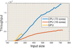
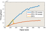
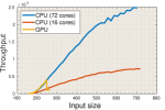
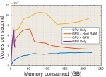
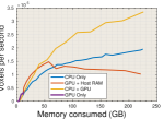
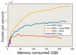
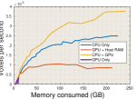
Fig. 5 shows the throughput achieved on the four benchmarked networks (Table III) with the batch size $S=1$, and different image sizes.

It turns out that the optimal choice for primitives for the CPU is always the same regardless of the network choice. In all cases the first (convolutional) layer was optimized to data–parallel FFT–based algorithm, and the rest of the convolutional layers used the task–based algorithm. This is expected because of the much higher cache locality of our FFT implementations compared to direct convolution, which plays an important role on the CPU with very fast cache access and relatively slow RAM access.

	n337	n537	n726	n926
Input size	$235^{3}$	$217^{3}$	$243^{3}$	$253^{3}$
Layer $1$	CuDNN1	CuDNN1	CuDNN1	CuDNN1
Layer $2$	MPF	MPF	MPF	MPF
Layer $3$	CuDNN2	FFT	FFT	CuDNN1
Layer $4$	MPF	MPF	MPF	MPF
Layer $5$	CuDNN2	CuDNN2	FFT	FFT
Layer $6$	MPF	MPF	FFT	FFT
Layer $7$	CuDNN2	CuDNN2	FFT	FFT
Layer $8$	CuDNN2	CuDNN2	FFT	FFT
Layer $9$	CuDNN2	CuDNN2
Layer $10$	CuDNN2	CuDNN2

TABLE IV: Optimal choice for different layers.

The optimal use of primitives for the GPU have higher dependence on the ConvNet’s architecture. The optimal choice of primitives for each network, as well as the optimal input image size is given in Table IV. Interestingly, the implementation for the first layer of all networks is the slower version of the cuDNN’s primitive. Even though the primitive is slower, it is able to process larger input image, as it has lower memory requirement. There is a trade–off between the layer speed, and the maximal size of the input that a layer can process. In this case it was more beneficial to be able to process larger inputs.

VII GPU + host RAM and CPU–GPU inference

We saw that the throughput can highly depend on the size of the input image we are able to process by the network. For kernels of size $5^{3}$ or more CPU seems to outperform GPU due to these limits. For that reason we introduce another layer primitive, a layer whose data is stored in host RAM, and is partially uploaded to the GPU where the computation is performed.

VII-A GPU + host RAM convolutional layer

(a)

(b)

Figure 6: Decomposing a convolutional layer into multiple convolutional sub–layers.

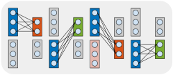
Consider a convolutional layer whose input is shape is $(S,f,x,y,z)$ and output shape $(S,f^{\prime},x^{\prime},y^{\prime},z^{\prime})$. The computation performed by the layer can be divided into $N$ sub–layers with input shapes of $(S_{i},f_{i},x,y,z)$ and output shape $(S_{i},f^{\prime}_{i},x^{\prime},y^{\prime},z^{\prime})$. Fig. 6 illustrates how the computation of a convolutional layer with $S=1$, $f=6$, and $f^{\prime}=4$ can be divided into $N=4$ sub–layers, each having $S_{i}=1$, $f_{i}=3$ and $f^{\prime}_{i}=2$. The blue color represents the input images that have to be transferred to the GPU, the red color represents the memory that has to be allocated on the GPU. The green color represent the results that have to be transferred back to the host. The computation of each sub–layer can be performed by any of the GPU–only primitives. The time required for processing the layer will equal to the sum of processing time of each sub–layer and the time required for memory transfers. Due to the GPU’s memory limit, not all divisions are feasible.

Due to a large number of possible divisions, simple way to find the optimal division into sub–layers by considering all feasible divisions, and then picking the optimal primitive for each sub–layer might be very time consuming. The search can be pruned using the following two heuristics.

First, for small kernel sizes ($5^{3}$ or smaller), we consider only the cuDNN primitives based on direct–convolution; and for larger kernels we only consider our FFT–based primitive.

Second, when $S>1$, we prefer the division into sub–layers such that $f_{i}=f$, $f^{\prime}_{i}=f^{\prime}$, and $S_{i}\leq S$. This, essentially divides the batches of the input into sub–batches that are processed on the GPU. In this case, each input will have to be transferred to the GPU exactly once, and each output will be transferred back to the host exactly once.

If there is no feasible division into sub–batches, we prefer sub–layers with $S_{i}=1$, where most of the sub–layers have $f_{i}=f_{\alpha}\leq f$ and $f^{\prime}_{i}=f^{\prime}_{\alpha}\leq f^{\prime}$. Some sub–layers will have to have a different input/output shape if $f$ or $f^{\prime}$ are not divisible by $f_{\alpha}$ and $f^{\prime}_{\alpha}$, respectively. As most of the sub–layers have the same input and output shape, the time required for the layer can be estimated by running only sub–layers with distinctive input shapes.

The two heuristics render the search for the optimal sub–division, and optimal choice for each sub–layer very fast.

The host memory requirement for this layer equals to the amount of memory required to store the input and the output tensor, and GPU on–board memory has to be large enough to facilitate each sub–layer.

VII-B GPU + host RAM ConvNet execution

Implementing GPU + host RAM MPF layer turned out to be impractical. Originally we implemented similar GPU + host RAM MPF layers. However, it turned out that it is better to compute the MPF layers on the CPU, even when very few cores are available. This is because of the expensive transfer to and from device and relative low computational complexity of the MPF layers.

(a)

(b)

(c)

(d)

Figure 7: Maximal throughput achieved vs memory consumption using GPU–only, CPU–only, CPU + host RAM and CPU–GPU implementations for different image sizes.

Figure 8: A network of form CPCPCCCC with the first half executed one layer at the time, and the second half one batch at the time. We pooling window size of the MPF layers is $2\times 1\times 1$.

The simplest way to execute a network using the GPU for computation and host RAM for storage is to use individually optimized GPU + host RAM layer described above for each convolutional layer, and the CPU implementation of a MPF layer for each pooling layer.

Turns out that, when using MPF layers for evaluating a max–pooling ConvNet we can achieve better performances by minimizing the data transferred to and from the GPU. To understand how we can improve the performances, we need to understand the following property of a ConvNet.

A ConvNet with input shape $I=(S,f,x,y,z)$ with $S>1$, will have the batch size $S^{\prime}$ of the output shape $I^{\prime}=(S^{\prime},f^{\prime},x^{\prime},y^{\prime},z^{\prime})$ always divisible by $S$. The values $I^{\prime}(\frac{S^{\prime}}{S}i:\frac{S^{\prime}}{S}(i+1),:,:,:,:)$ will only depend on $I(i,:,:,:,:)$. This means that concatenating results of applying a layer on two inputs $I_{1}(S_{1},f,x,y,z)$ and $I_{2}(S_{2},f,x,y,z)$ will equal to the result of the concatenated input of size $(S_{1}+S_{2},f,x,y,z)$.

Network	Baseline (cuDNN)	Caffe	ELEKTRONN	ZNN	GPU-Only	CPU-Only	GPU + host RAM	GPU-CPU
n337	$22,934.8$	$1.348$	$122,668$	$34,334.8$	$671,782$	$262,131$	$727,103$	$1,059,910$
n537	$1,048.68$	–	–	$9,494.5$	$29,352.1$	$194,683$	$147,965$	$334,163$
n726	$13,520.4$	–	$6,122$	$31,354.8$	$97,257.2$	$300,312$	$148,194$	$470,166$
n926	$2,667.86$	–	–	$20,908.6$	$35,051.3$	$249,190$	$104,946$	$375,295$

TABLE V: Comparisons to other methods.

Consider the output shape of the first $\theta$ layers of a ConvNet. The computation of the rest of the layers can be considered to be another ConvNet that takes the output of the $\theta^{th}$ layer as the input. If some of the first $\theta$ layers were MPF layers, the batch size of the $\theta^{th}$ layer output $S_{\theta}$ will be greater than 1. Instead processing one layer at the time for the rest of the layers, one might be able to process all remaining layers for a sub–batch $\hat{S}_{\theta}$ at the time using a GPU–only network. This will reduce the memory transfer overhead as no intermediate results have to be transferred back to the host. In Fig. 8 we illustrate the timeline of executing a network of the form CPCPCCCC by having the first four layers executed one layer at the time, and the rest one batch at the time.

We illustrate the stragety through the follwing example. Assume we are given a ConvNet architecture in the form CPCPCCCC, where each layer has 3 input and 3 output images, except for the first layer that has 1 input image and the last that has 1 output image. Let the sizes of the pooling window be $2\times 1\times 1$, this means that when MPF layers is used, for each input tuple a MPF layer will produce 2 fragments of the same size. Mainly the most significant dimension of the input tensor to the layer will double. If the batch size $S$ of the network input was $1$, the output of the second MPF layer will have the batch size of $4$. At this point we might be able to process the rest of the network for a single input tuple (or multiple) using the GPU–only approach, thus only having to upload the input to the GPU once, and fetch the final result once. Processing the first four layers of the network using the GPU + host RAM and MPF layers and the rest of the layers with the GPU–only approach for the rest of the ConvNet is illustrated in Fig. 8. Here we process the first four layers, one layer at the time, and the last four layers one batch at the time.

Finding the optimal network execution strategy for such execution becomes more complex. The first additional parameter we have is $\theta$, $(0\leq\theta\leq L)$, where $L$ is the number of layers of the given ConvNet. This parameters represent the number of layers that will be processed one at the time using the GPU + host RAM or CPU-MPF layer at the time. The rest of the network is then executed one (or more) batches at the time using the GPU–only primitives.

For a given value of $\theta$ and a given input size, this approach has two limitations. Firstly, $\theta$ layers have to fit on the host RAM. Secondly, there has to exist a GPU–only network that can process the latter layers on the GPU.

In order to find an optimal implementation we, consider any valid input shape and any valid $\theta$ that are convolutional to use GPU + host RAM primitive, and separately optimize the rest of the GPU–only network

VII-C CPU–GPU ConvNet execution

Finally, inference can be done by utilizing both CPU and GPU. As in the GPU + host RAM approach, the network layers are divided into two groups. For the first $\theta$ layers, we use the optimal CPU implementation as defined in Section VI, and for the rest of the layers we use the optimal GPU implementation as defined in the previous section.

The CPU and the GPU form a producer–consumer pipeline. The CPU produces by computing the first $\theta$ layers for a given input image, and queuing the result. The GPU consumes the data on the queue, taking as input the output of the $\theta^{th}$ layer, and yields the final output of the last layer.

This approach can generate huge memory overhead if the CPU produces data much faster than the GPU can consume. For that reason, the CPU is not allowed to start working on the next input until the queue is empty – until the GPU had picked up and started executing the rest of the network for all the data on the queue. This essentially limits the queue to a maximal size of one.

For a given value of $\theta$ and a given input size the GPU will operate on the output of the $\theta^{th}$ layer producing the final output. Hence the output of the $\theta^{th}$ layer has to be stored in the host RAM, along with memory allocated for the network output. As both the CPUs and GPUs can do work only when the queue is empty, the rest of the host RAM is available to the CPUs.

Finding the optimal implementation through an exhaustive search resembles the one in the previous section. For each valid input shape, we loop over all valid values of $\theta$, and for each such division of the ConvNet, we separately optimize the first $\theta$ CPU-only layers and the rest of the GPU-only layers, having the memory limitations in mind.

Fig. 7 shows the throughput achieved on the four benchmarked networks (Table III) with the batch size $S=1$, and different image sizes obtained during the exhaustive search for the highest throughput. Instead of showing the input image size on the $x$ axis, we decide to show the memory required by the implementation, as it allows us to analyze how the memory available to the system influences the maximal possible throughput. The memory consumed is calculated as $\max\{M_{CPU},M_{GPU}\}$.

VIII Comparison to other algorithms

We compare our 4 approaches (GPU–only, CPU–only, GPU + host RAM and GPU–CPU) with other publicly available implementations and show the results in the Table V. All benchmarks are performed on the same hardware, the 4–way Intel Xeon E7–-8890 v3 machine with 256GB of RAM and a Titan X GPU.

The results of our approaches are based on the optimizations described in the previous sections. For the other approaches, we varied the input sizes and measured the throughput, we reported the highest value of throughput obtained, which was always correlated with the size of the input we were able to process.

The baseline (cuDNN) approach consists of calling the cuDNN [29] primitives for convolution and max–pooling. Unlike other approaches, this is not a general framework – it requires the user to write some code for calling into the cuDNN primitives, for calculating the input/output shapes and some minimal memory management. We expect that a user with minimal programming experience could implement the above. Our implementation was done in C++, however one could use cuDNN bindings for other languages.

Caffe [30] is another GPU ConvNet framework. We benchmarked a version that implements sliding window ConvNets using “strided kernels” [11]. The implementation is also optimized for training and seems to have a huge memory overhead as we were only able to run the smallest of the networks.

ELEKTRONN [12] was the only competitor that provides inference optimization for 3D sliding window ConvNets using MPF. The package also uses cuDNN convolutional primitives. However, it was able only to process two of our four networks.

ZNN [10] is a framework optimized for training sliding window 3D ConvNets on multi–core and many–core CPUs using “max–filtering” followed by FFT–based “sparse convolution”. ZNN was the best competitor for networks with filters of $5\times 5\times 5$ or larger.

Our CPU-only, GPU-only, GPU + host RAM, and CPU-GPU implementations outperform all competitors. For the smallest ConvNet architecture, 237 with the kernel sizes of $3^{3}$, the next best competitor was ELEKTRONN with approximately a tenth of the speed of our CPU–GPU approach. For all the other ConvNets, the next best competitor was ZNN with approximately $15\times$ smaller throughput.

References

- [1] K. Chellapilla, S. Puri, and P. Simard, “High performance convolutional neural networks for document processing,” in Tenth International Workshop on Frontiers in Handwriting Recognition. Suvisoft, 2006.
- [2] D. Scherer, H. Schulz, and S. Behnke, “Accelerating large-scale convolutional neural networks with parallel graphics multiprocessors,” in Artificial Neural Networks–ICANN 2010. Springer, 2010, pp. 82–91.
- [3] D. Strigl, K. Kofler, and S. Podlipnig, “Performance and scalability of gpu-based convolutional neural networks,” in 2010 18th Euromicro Conference on Parallel, Distributed and Network-based Processing. IEEE, 2010, pp. 317–324.
- [4] D. C. Ciresan, U. Meier, J. Masci, L. Maria Gambardella, and J. Schmidhuber, “Flexible, high performance convolutional neural networks for image classification,” in IJCAI Proceedings-International Joint Conference on Artificial Intelligence, vol. 22, no. 1, 2011, p. 1237.
- [5] M. Meeker, “Internet trends 2014,” \urlhttp://www.kpcb.com/blog/2014-internet-trends, 2014 (accessed April 9, 2016).
- [6] “Youtube changes at a rate of 33% a year.”
- [7] J. W. Lichtman, H. Pfister, and N. Shavit, “The big data challenges of connectomics,” Nature neuroscience, vol. 17, no. 11, pp. 1448–1454, 2014.
- [8] M. Mathieu, M. Henaff, and Y. LeCun, “Fast training of convolutional networks through ffts,” in International Conference on Learning Representations (ICLR2014). CBLS, April 2014.
- [9] N. Vasilache, J. Johnson, M. Mathieu, S. Chintala, S. Piantino, and Y. LeCun, “Fast convolutional nets with fbfft: A gpu performance evaluation,” arXiv preprint arXiv:1412.7580, 2014.
- [10] A. Zlateski, K. Lee, and H. S. Seung, “Znn-a fast and scalable algorithm for training 3d convolutional networks on multi-core and many-core shared memory machines,” arXiv preprint arXiv:1510.06706, 2015.
- [11] F. Tschopp, “Efficient convolutional neural networks for pixelwise classification on heterogeneous hardware systems,” arXiv preprint arXiv:1509.03371, 2015.
- [12] M. P. I. F. M. Research. (2015) ELEKTRONN a neural network toolkit. [Online]. Available: \urlhttp://elektronn.org/
- [13] O. Matan, C. J. Burges, Y. LeCun, and J. S. Denker, “Multi-digit recognition using a space displacement neural network,” in NIPS. Citeseer, 1991, pp. 488–495.
- [14] P. Sermanet, D. Eigen, X. Zhang, M. Mathieu, R. Fergus, and Y. LeCun, “Overfeat: Integrated recognition, localization and detection using convolutional networks,” arXiv preprint arXiv:1312.6229, 2013.
- [15] V. Jain, J. F. Murray, F. Roth, S. Turaga, V. Zhigulin, K. L. Briggman, M. N. Helmstaedter, W. Denk, and H. S. Seung, “Supervised learning of image restoration with convolutional networks,” in Computer Vision, 2007. ICCV 2007. IEEE 11th International Conference on. IEEE, 2007, pp. 1–8.
- [16] F. Ning, D. Delhomme, Y. LeCun, F. Piano, L. Bottou, and P. E. Barbano, “Toward automatic phenotyping of developing embryos from videos,” Image Processing, IEEE Transactions on, vol. 14, no. 9, pp. 1360–1371, 2005.
- [17] A. Giusti, D. C. Cireşan, J. Masci, L. M. Gambardella, and J. Schmidhuber, “Fast image scanning with deep max-pooling convolutional neural networks,” arXiv preprint arXiv:1302.1700, 2013.
- [18] J. Masci, A. Giusti, D. Ciresan, G. Fricout, and J. Schmidhuber, “A fast learning algorithm for image segmentation with max-pooling convolutional networks,” in Image Processing (ICIP), 2013 20th IEEE International Conference on. IEEE, 2013, pp. 2713–2717.
- [19] F. Yu and V. Koltun, “Multi-scale context aggregation by dilated convolutions,” arXiv preprint arXiv:1511.07122, 2015.
- [20] J. Long, E. Shelhamer, and T. Darrell, “Fully convolutional networks for semantic segmentation,” in The IEEE Conference on Computer Vision and Pattern Recognition (CVPR), June 2015.
- [21] M. Frigo and S. G. Johnson, “Fftw user’s manual,” Massachusetts Institute of Technology, 1999.
- [22] ——, “Fftw: An adaptive software architecture for the fft,” in Acoustics, Speech and Signal Processing, 1998. Proceedings of the 1998 IEEE International Conference on, vol. 3. IEEE, 1998, pp. 1381–1384.
- [23] C. Nvidia, “Cufft library,” 2010.
- [24] H. S. Warren, Hacker’s delight. Pearson Education, 2013.
- [25] N. Bell and J. Hoberock, “Thrust: A 2 6,” GPU Computing Gems Jade Edition, p. 359, 2011.
- [26] J. Jeffers and J. Reinders, High Performance Parallelism Pearls Volume Two: Multicore and Many-core Programming Approaches. Morgan Kaufmann, 2015.
- [27] J. Reinders, Intel threading building blocks: outfitting C++ for multi-core processor parallelism. ” O’Reilly Media, Inc.”, 2007.
- [28] T. Willhalm and N. Popovici, “Putting intel® threading building blocks to work,” in Proceedings of the 1st international workshop on Multicore software engineering. ACM, 2008, pp. 3–4.
- [29] S. Chetlur, C. Woolley, P. Vandermersch, J. Cohen, J. Tran, B. Catanzaro, and E. Shelhamer, “cudnn: Efficient primitives for deep learning,” arXiv preprint arXiv:1410.0759, 2014.
- [30] Y. Jia, E. Shelhamer, J. Donahue, S. Karayev, J. Long, R. Girshick, S. Guadarrama, and T. Darrell, “Caffe: Convolutional architecture for fast feature embedding,” in Proceedings of the ACM International Conference on Multimedia. ACM, 2014, pp. 675–678.