Reducing bias and MSE in estimation of heavy tails:
a Bayesian approach

Abstract

Bias reduction in tail estimation has received considerable interest in extreme value analysis. Estimation methods that minimize the bias while keeping the mean squared error (MSE) under control, are especially useful when applying classical methods such as the Hill (1975) estimator. In Caeiro et al. (2005) minimum variance reduced bias estimators of the Pareto tail index were first proposed where the bias is reduced without increasing the variance with respect to the Hill estimator. This method is based on adequate external estimation of a pair of second-order parameters. Here we revisit this problem from a Bayesian point of view starting from the extended Pareto distribution (EPD) approximation to excesses over a high threshold, as developed in Beirlant et al. (2009) using maximum likelihood (ML) estimation. Using asymptotic considerations, we derive an appropriate choice of priors leading to a Bayes estimator for which the MSE curve is a weighted average of the Hill and EPD-ML MSE curves for a large range of thresholds, under the same conditions as in Beirlant et al. (2009). A similar result is obtained for tail probability estimation. Simulations show surprisingly good MSE performance with respect to the existing estimators.

Keywords: Extended Pareto Distribution, Peaks over threshold, extreme value index, Bayesian parameter estimation, bias reduction, posterior simulation.

1 Introduction

In this paper we consider the estimation of the extreme value index $\xi$ and tail probabilities $P(X>x)$ for $x$ large, on the basis of independent and identically distributed observations $X_{1},X_{2},\ldots,X_{n}$ which follow a Pareto-type distribution with right tail function (RTF) given by

$$\bar{F}(x)=1-F(x)=P(X>x)=x^{-1/\xi}\ell(x)$$ (1)

where $\ell$ is a slowly varying function at infinity, i.e.

$${\ell(ty)\over\ell(t)}\to 1,\mbox{ as }t\to\infty,\mbox{ for every }y>1.$$

The most famous estimator of $\xi$ was first derived by Hill (1975) as a maximum likelihood (ML) estimator using the approximation

$$\bar{F}(ty)/\bar{F}(t)\approx y^{-1/\xi},t\mbox{ large}$$ (2)

to the RTF of the excesses $X/t|X>t$ over a large threshold $t$ by a simple Pareto distribution with RTF $y^{-1/\xi}$, and setting $t=X_{n-k,n}$ where $X_{1,n}\leq X_{2,n}\leq\ldots\leq X_{n,n}$:

$$H_{k,n}={1\over k}\sum_{j=1}^{k}\log{X_{n-j+1,n}\over X_{n-k,n}}.$$ (3)

A simple estimator of a tail probability $P(X>x)$ with $x$ large, introduced in Weissman (1978),
is then obtained from (2) setting $ty=x$ and estimating $P(X>t)$ by the empirical proportion $k/n$:

$$\hat{p}_{x,k}={k\over n}\left({x\over X_{n-k,n}}\right)^{-1/H_{k,n}}.$$ (4)

In practice, a way to verify the validity of model (1) is to check whether the Hill estimates are stable as a function of $k$. However in most cases the stability is not visible, which can be explained by slow convergence in (2). For this reason bias reduced estimators have been proposed which lead to plots that are much more horizontal in $k$ which facilitates the analysis of a practical case to a great extent. Here we can refer to Peng (1998), Beirlant et al. (1999, 2008), Feuerverger and Hall (1999), Caeiro et al. (2005, 2009) and Gomes et al. (2007) for bias-reduced estimators based on functions of the top $k$ order statistics. Several of these methods focus on the distribution of log-spacings of high order statistics.

Beirlant et al. (2009) proposed to build a more flexible model capable of capturing the deviation between the true excess RTF $\bar{F}(ty)/\bar{F}(t)$ and the asymptotic Pareto model. For a heavy tailed distribution (1), this deviation can be parametrized using a power series expansion (Hall, 1982), or more generally via second-order slow variation (Bingham et al., 1987). More specifically in Beirlant et al. (2009) the subclass $\mathcal{F}(\xi,\tau)$ of the Pareto-type tails (1) was considered satisfying

$$\bar{F}(x)=Cx^{-1/\xi}\left(1+\xi^{-1}\delta(x)\right),$$ (5)

with $\delta(x)$ eventually nonzero and of constant sign such that $|\delta(x)|=x^{\tau}\ell_{\delta}(x)$ with $\tau<0$ and $\ell_{\delta}$ slowly varying. It was shown that under $\mathcal{F}(\xi,\tau)$ one has as $t\to\infty$

$$\sup_{y\geq 1}\left|{\bar{F}(ty)\over\bar{F}(t)}-\bar{G}_{\xi,\delta,\tau}(y)\right|=o\left(|\delta(t)|\right)$$

with $\bar{G}_{\xi,\delta,\tau}$ the RTF of the extended Pareto distribution (EPD)

$$\bar{G}_{\xi,\delta,\tau}(y)=\{y(1+\delta-\delta y^{\tau})\}^{-1/\xi},\ \ \ y>1,$$ (6)

with $\tau<0<\xi$ and $\delta>\max(-1,1/\tau)$. This shows that the EPD improves the approximation (2) with an order of magnitude. Then maximum likelihood (ML) estimation of the parameters ($\xi,\delta$) based on a set of excesses $\left(Y_{j,k}:=X_{n-j+1,n}/X_{n-k,n},\;j=1,\ldots,k\right)$ was used to obtain a bias reduced estimator of $\xi$. Bias reduction of the Weissman estimator of tail probabilities can analogously be obtained using

$$\hat{p}^{EP}_{x,k}={k\over n}\bar{G}_{\hat{\xi}_{k},\hat{\delta}_{k},\hat{\tau}}\left({x\over X_{n-k,n}}\right),$$ (7)

where $(\hat{\xi}_{k},\hat{\delta}_{k})$ denote the ML estimators based on the EPD model, and where $\hat{\tau}$ is a consistent estimator of $\tau$, to be specified below, which was shown not to affect the asymptotic distribution of $(\xi,\delta)$.

Here we investigate the possibilities of using the Bayesian methodology when modelling the distribution of the vector of excesses ${\bf Y}_{k}:=\left(Y_{j,k},j=1,\ldots,k\right)$ with an EPD. In section 2 we show that a normal prior on $\delta$ with zero mean and variance $\sigma^{2}_{k,n}$, depending in an appropriate way on $k$ and $n$, leads to interesting MSE results of the posterior mode estimators for $\xi$ and of the corresponding estimators of $P(X>x)$ following (7). In section 3 we discuss the implementation of the Bayesian estimates. In section 4 we consider the finite sample behaviour of this Bayesian approach and consider some practical cases.

2 Bayesian estimation of the EPD parameters

ML estimation of the EPD parameters ($\xi,\delta$), given a value of $\tau$, follows by maximizing the log-likelihood

$${1\over k}l(\xi,\delta|{\bf y})=-\log\xi-(\frac{1}{\xi}+1){1\over k}\sum_{j=1}^{k}\left[\log y_{j,k}+\log(1+\delta\{1-y_{j,k}^{\tau}\})\right]+{1\over k}\sum_{j=1}^{k}\log\left(1+\delta\{1-(1+\tau)y_{j,k}^{\tau}\}\right).$$ (8)

In the Bayesian framework, the log-posterior can be written as

$${1\over k}\log\pi(\xi,\delta|{\bf y})={1\over k}l(\xi,\delta|{\bf y})+{1\over k}\log\pi(\xi,\delta),$$ (9)

where $\pi(\xi,\delta)$ denotes the prior density. Here we assign a maximal data information (MDI) prior to $\xi$, which for a general parameter $\theta$ is defined as $\pi(\theta)\propto\exp(E(\log f({\bf Y}|\theta)))$. Beirlant et al. (2004) derived that the MDI for a Pareto distribution is given by

$$\pi(\xi)\propto\frac{e^{-\xi}}{\xi}.$$ (10)

Next, the prior on $\delta$ is taken to be a normal distribution with mean 0 and variance $\sigma^{2}_{k,n}$, depending on $k$, and left truncated in order to comply with the restriction $\delta>\max(-1,1/\tau)$:

$$\pi(\delta)={1\over\sqrt{2\pi}\sigma_{k,n}}e^{-{1\over 2}{\delta^{2}\over\sigma^{2}_{k,n}}}/\left(1-\Phi(\max(-1,\tau^{-1})/\sigma_{k,n})\right).$$ (11)

If $F$ satisfies $\mathcal{F}(\xi,\tau)$, it is shown in Beirlant et al. (2009) that $Q(1-x^{-1})$ ($x>1$), with $Q(p)=\inf\{x:F(x)\geq p\}$ ($p\in(0,1)$), satisfies

$$Q(1-x^{-1})=C^{\xi}x^{\xi}\left(1+a(x)\right)$$ (12)

with $a(x)=\delta(Q(1-x^{-1}))\{1+o(1)\}=\delta(C^{\xi}x^{\xi})\{1+o(1)\}$ as $x\to\infty$. In particular $a$ is eventually nonzero and of constant sign and $|a(x)|=x^{\rho}\ell_{a}(x)$ with $\ell_{a}$ slowly varying and $\rho=\xi\tau$.

Then it was shown that if $F$ satisfies $\mathcal{F}(\xi,\tau)$, and $\sqrt{k}a(n/k)\to\lambda\in\mathbb{R}$ and $\hat{\rho}_{n}=\rho+o_{p}(1)$ as $k,n\to\infty$ and $k/n\to 0$, the following asymptotic results hold for the EPD-ML estimator $\hat{\xi}^{ML}_{k,n}$ and $H_{k,n}$:

$$\sqrt{k}\left(\hat{\xi}^{ML}_{k,n}-\xi\right) \to_{d} \mathcal{N}\left(0,\xi^{2}\left({1-\rho\over\rho}\right)^{2}\right),$$ (13)

$$\sqrt{k}\left(H_{k,n}-\xi\right) \to_{d} \mathcal{N}\left(\lambda{\rho\over 1-\rho},\xi^{2}\right).$$ (14)

From these results it follows that for the smallest values of $k$ (i.e. $\sqrt{k}a(n/k)\to 0$) the Hill estimator is asymptotically unbiased, while for increasing values of $k$ (i.e. $\sqrt{k}a(n/k)\to\lambda\neq 0$) it is biased. In this region the bias reduced estimator $\hat{\xi}^{ML}_{k,n}$ still has asymptotic bias 0, but its variance is increased by a factor $((1-\rho)/\rho)^{2}$ compared to $H_{k,n}$.

In the Appendix we derive that the first order approximations ($\hat{\xi}_{k}^{\mathcal{B}},\hat{\delta}_{k}^{\mathcal{B}}$) of the Bayesian estimators are given by

$$\hat{\xi}_{k}^{\mathcal{B}} = H_{k,n}+\hat{\delta}_{k}^{\mathcal{B}}\left(1-E_{k,n}(\tau)\right),$$

$$\hat{\delta}_{k}^{\mathcal{B}} = \frac{1-H_{k,n}\tau}{D^{\mathcal{B}}_{k,n}}\left(E_{k,n}(\tau)-{1\over H_{k,n}\tau}\right)$$

where

$$E_{k,n}(s)={1\over k}\sum_{j=1}^{k}Y_{j,k}^{s},\;s<0,$$

and

$$D^{\mathcal{B}}_{k,n}={\hat{\xi}_{k}^{\mathcal{B}}\over k\sigma^{2}_{k,n}}-\left(1-2(1-\hat{\xi}_{k}^{\mathcal{B}}\tau)E_{k,n}(\tau)+(1-2\hat{\xi}_{k}^{\mathcal{B}}\tau-\hat{\xi}_{k}^{\mathcal{B}}\tau^{2})E_{k,n}(2\tau)-\tau(1-E_{k,n}(\tau))E_{k,n}(\tau)\right).$$

These expressions are identical to the asymptotic EPD-ML estimators derived in Beirlant et al. (2009) except for the extra term ${\hat{\xi}_{k}^{\mathcal{B}}\over k\sigma^{2}_{k,n}}$ in the expression of $D^{\mathcal{B}}_{k,n}$. As an external estimator of $\tau$ we use $\hat{\tau}=\hat{\rho}/H_{k,n}$ where $\hat{\rho}$ is a consistent estimator of $\rho$ (see for instance $\rho_{Fraga}$ from Fraga Alves et al., 2003). The following result is derived in the Appendix.

Theorem. Let $F\in\mathcal{F}(\xi,\tau)$ and assume $k\sigma_{k,n}^{2}\to\mu>0$ as $k,n\to\infty$, $k/n\to 0$ and $\sqrt{k}a(n/k)\to\lambda$. Then $\Xi_{k,n}:=\sqrt{k}\left(\hat{\xi}_{k}^{\mathcal{B}}-\xi\right)$ is asymptotically normal with asymptotic mean and variance given by

$$E_{\infty}(\Xi_{k,n}) = {\lambda\rho\over 1-\rho}{\zeta\over\zeta+\rho^{4}},$$ (15)

$$Var_{\infty}(\Xi_{k,n}) = {\xi^{2}\over(1+\zeta\rho^{-4})^{2}}\left(\left({1-\rho\over\rho}\right)^{2}+{\zeta^{2}\over\rho^{8}}+2{\zeta\over\rho^{4}}\right).$$ (16)

Minimizing $MSE_{\infty}(\Xi_{k,n})=E^{2}_{\infty}(\Xi_{k,n})+Var_{\infty}(\Xi_{k,n})$ with respect to $\zeta$ leads to

$$\zeta_{opt}={\xi^{2}(1-2\rho)\over\lambda^{2}},$$ (17)

from which, with $\zeta_{opt}=\xi^{2}(1-2\rho)(1-\rho)^{2}/\mu_{opt}$,

$$\mu_{opt}=(1-\rho)^{2}\lambda^{2}.$$ (18)

Hence, we are lead to choosing

$$\sigma^{2}_{opt,k,n}=(1-\rho)^{2}a^{2}(n/k)$$ (19)

for the prior variance since $\mu=\lim_{k,n\to\infty}k\sigma^{2}_{k,n}$ and $\lambda^{2}=\lim_{k,n\to\infty}ka^{2}(n/k)$.

Note that using (17), one obtains from (15) and (16) that

$$E^{opt}_{\infty}(\Xi_{k,n}) = {\lambda\rho\over 1-\rho}{\xi^{2}(1-2\rho)\over\xi^{2}(1-2\rho)+\lambda^{2}\rho^{4}},$$

$$Var^{opt}_{\infty}(\Xi_{k,n}) = {\xi^{2}\lambda^{4}\over(\lambda^{2}\rho^{4}+\xi^{2}(1-2\rho))^{2}}\left\{(1-\rho)^{2}\rho^{6}+\lambda^{-4}\xi^{4}(1-2\rho)^{2}+2\lambda^{-2}\xi^{2}(1-2\rho)\rho^{4}\right\},$$

from which

$$MSE^{opt}_{\infty}(\Xi_{k,n}) = \frac{\xi^{4}(1-2\rho)^{2}[\xi^{2}+\lambda^{2}{\rho^{2}\over(1-\rho)^{2}}]+2\xi^{2}\rho^{4}\lambda^{2}(1-2\rho)[\xi^{2}]+\lambda^{4}\rho^{8}[\xi^{2}{(1-\rho)^{2}\over\rho^{2}}]}{\xi^{4}(1-2\rho)^{2}+2\xi^{2}\rho^{4}\lambda^{2}(1-2\rho)+\lambda^{4}\rho^{8}}$$ (20)

$$= \xi^{2}+\xi^{2}\rho^{2}{(1-2\rho)\over(1-\rho)^{2}}\,\lambda^{2}\,\frac{\left(\xi^{2}(1-2\rho)+\lambda^{2}\rho^{4}(1-\rho)^{2}\right)}{(\xi^{2}(1-2\rho)+\lambda^{2}\rho^{4})^{2}}.$$ (21)

From (20) it follows that the asymptotic MSE of this optimal Bayesian estimator is a weighted average of the asymptotic MSEs of the Hill and EPD-ML estimators. Moreover, since the right hand side of (21) is an increasing function in $\lambda^{2}$ it follows that

$$MSE^{opt}_{\infty}(\Xi_{k,n})\leq\lim_{\lambda\to\infty}MSE^{opt}_{\infty}(\Xi_{k,n})=MSE_{\infty}\left(\sqrt{k}(\hat{\xi}_{k,n}^{ML}-\xi)\right).$$

Also, expanding the the right hand side of (21) for $\lambda^{2}\to 0$ leads to

$$MSE^{opt}_{\infty}(\Xi_{k,n})=\xi^{2}+\lambda^{2}{\rho^{2}\over(1-\rho)^{2}}(1+o(1)).$$

We can conclude that the asymptotic MSE of the optimal Bayes estimator is uniformly smaller than the MSE of the EPD-ML estimator as given in (13), while for smaller $\lambda$ this asymptotic MSE follows the asymptotic MSE of the Hill estimator, given in (14), up to terms of order $\lambda^{2}$. Hence with the choice (19) the Bayesian estimator automatically follows the better of the two existing estimators as a function of $\lambda$ or $k$.

Replacing ($\hat{\xi}_{k},\hat{\delta}_{k}$) by ($\hat{\xi}^{\mathcal{B}}_{k},\hat{\delta}^{\mathcal{B}}_{k}$) in $\hat{p}^{EP}_{x,k}$, it follows from the proof of Theorem 5.2 in Beirlant et al. (2009) that the resulting tail probability estimator $\hat{p}^{\mathcal{B}}_{x,k}$ satisfies the following asymptotic result under the conditions of the Theorem:
when $p_{n}=P(X>x_{n})$ satisfies $np_{n}/k\to 0$ and $\log(np_{n})/\sqrt{k}\to 0$, then

$${\sqrt{k}\over\log(k/(np_{n}))}\xi({\hat{p}^{\mathcal{B}}_{x_{n},k}\over p_{n}}-1)$$

is asymptotically normal with the same limit distribution as in the Theorem. Hence the asymptotic MSE behaviour for the tail probability estimator has the same characteristics as the tail index estimator.

In the popular special case which contains most Pareto-type distributions (Hall, 1982) where for some constant $C$

$$x^{-\rho}a(x)\to_{x\to\infty}C,$$ (22)

the limit $C$ can be incorporated in $\lambda$ so that under (22) the variance of the normal prior on $\delta$ can be taken as

$$\sigma^{2}_{*,k,n}=\left({k\over n}\right)^{-2\hat{\rho}}.$$ (23)

This is the choice of $\sigma^{2}_{k,n}$ we will use throughout in practice, with $\rho$ estimated by the method proposed in Fraga Alves (2003). We will also study the sensitivity of the method when replacing $\rho$ by $-1$, as used for instance in Beirlant et al. (2002).

Denoting the Bayesian estimators of ($\xi,\delta$) using (23) by $(\hat{\xi}_{k,n}^{*},\hat{\delta}_{k,n}^{*})$, as in (7) we then find the corresponding estimator for tail probabilities $P(X>x)$:

$$\hat{p}^{*}_{x,k}={k\over n}\bar{G}_{(\hat{\xi}^{*}_{k,n},\hat{\delta}^{*}_{k,n},\hat{\rho}/H_{k,n})}\left({x\over X_{n-k,n}}\right).$$ (24)

3 Implementation of the Bayes estimators

Bayesian inference has a great advantage of incorporating in a unified way, any meaningful piece of information in describing our model parameters. Here we use the objective mathematical information that with decreasing $k$ (or increasing threshold $t$) the $\delta$ parameter becomes smaller, expressed by the variance of the normal prior on this parameter which is taken to be of order $(k/n)^{-2\rho}$. We rely on modern Markov Chain Monte Carlo (MCMC) methods to assist in approximating posterior distributions. In order to make inference on $(\xi,\delta)$ we take the mode of the posterior samples, and the accuracy of this inference is described by the posterior distribution itself through the highest posterior density (HPD) region. The HPD for $\xi$ represents a set of most probable values of the $\hat{\xi}$, constituting $100(1-\alpha)\%$ of the posterior mass. The HPD also has the characteristic that the density within the HPD region is never lower than the values outside.

The Bayesian estimations are implemented via OpenBUGS (an open source version of BUGS) in the R (R Core Team, 2014) statistical software.

In OpenBUGS we need to specify the EPD model likelihood, the parameter priors and starting values, then a Markov chain simulation is automatically implemented for the resulting posterior distribution given in (9). The EPD is however not included in the standard distributions list available in OpenBUGS, and we therefore indirectly implement the EPD model likelihood using a Poisson distribution.

Let $l_{i}=\frac{1}{k}l(\xi,\delta|y_{i})$, where $\frac{1}{k}l(\xi,\delta|y_{1},...,y_{n})$ is the EPD log-likelihood defined in (8). The EPD model likelihood can be written as

$$f(\textbf{y}|\xi,\delta)=\prod_{i=1}^{n}e^{l_{i}}=\prod_{i=1}^{n}\frac{e^{-(-l_{i})}(-l_{i})^{0}}{0!}=\prod_{i=1}^{n}f_{P}(0;-l_{i}).$$ (25)

The resulting density $f_{P}(0;-l_{i})$ therefore is a product of Poisson distributed pseudo random variables with mean equal to the EPD log-likelihood and with all observed values set equal to zero. This is known as the ‘Zero trick’ (Lunn et al., 2012). A positive constant $C$ is added to the mean to ensure that the mean of the pseudo random variables is positive. The resulting likelihood becomes

$$f(\textbf{y}|\xi,\delta)=\prod_{i=1}^{n}\frac{e^{-(-l_{i}+C)}(-l_{i}+C)^{0}}{0!}=\prod_{i=1}^{n}f_{P}(0;-l_{i}+C);$$ (26)

where $C$ is chosen such that $-l_{i}+C>0\mbox{ for }i=1,2,...,n$.

In BUGS the full probability model needs to be defined and hence all prior distributions need to be proper (i.e. integrate to 1). The left truncated normal prior on $\delta$ is proper and can be specified directly in OpenBUGS. To ensure the MDI Pareto prior on $\xi$ is proper, we write it as

$$\pi(\xi)\propto\frac{e^{-\xi}}{\xi}\propto\frac{1}{\Gamma(\alpha)}\xi^{\alpha-1}e^{-\xi}.$$ (27)

and specify it in OpenBUGS using a Gamma distribution with a scale parameter equal to 1 and a shape parameter equal to 0.0001.

Values of $\rho$ close to 0 have to be avoided, and so we put a restriction on $\rho_{Fraga}$ in our implementation, using $\hat{\rho}=\min(-0.5,\rho_{Fraga})$. Finally we also smooth the Bayesian estimates as a function of $k$ with a moving average with a window width of 5.

4 Simulations and practical case studies

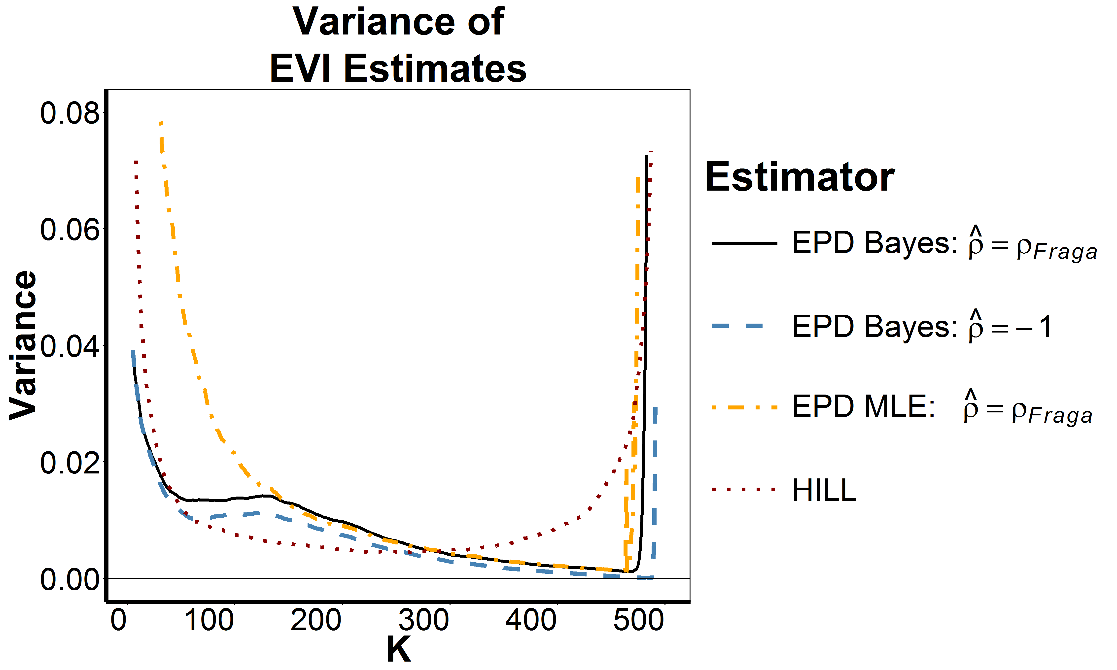
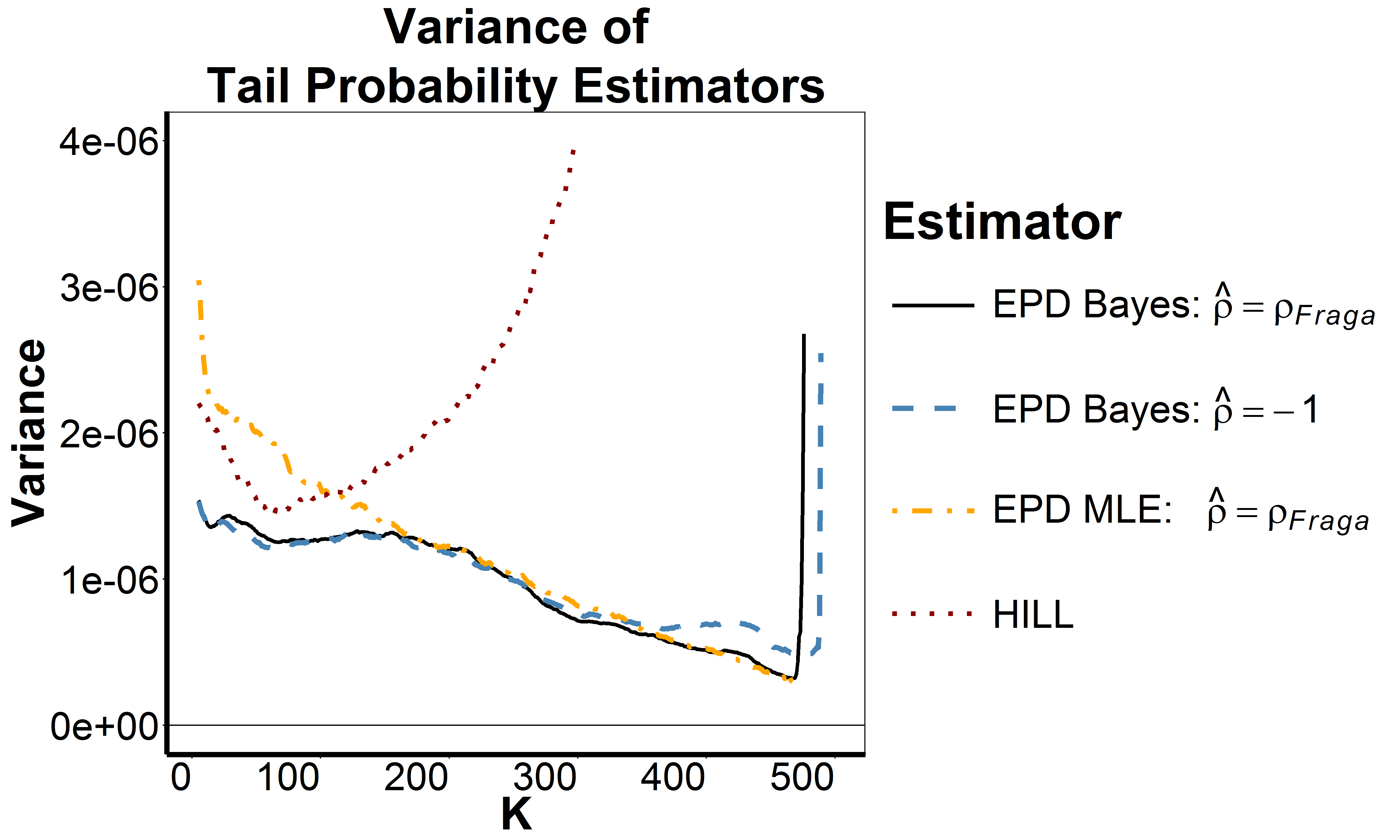
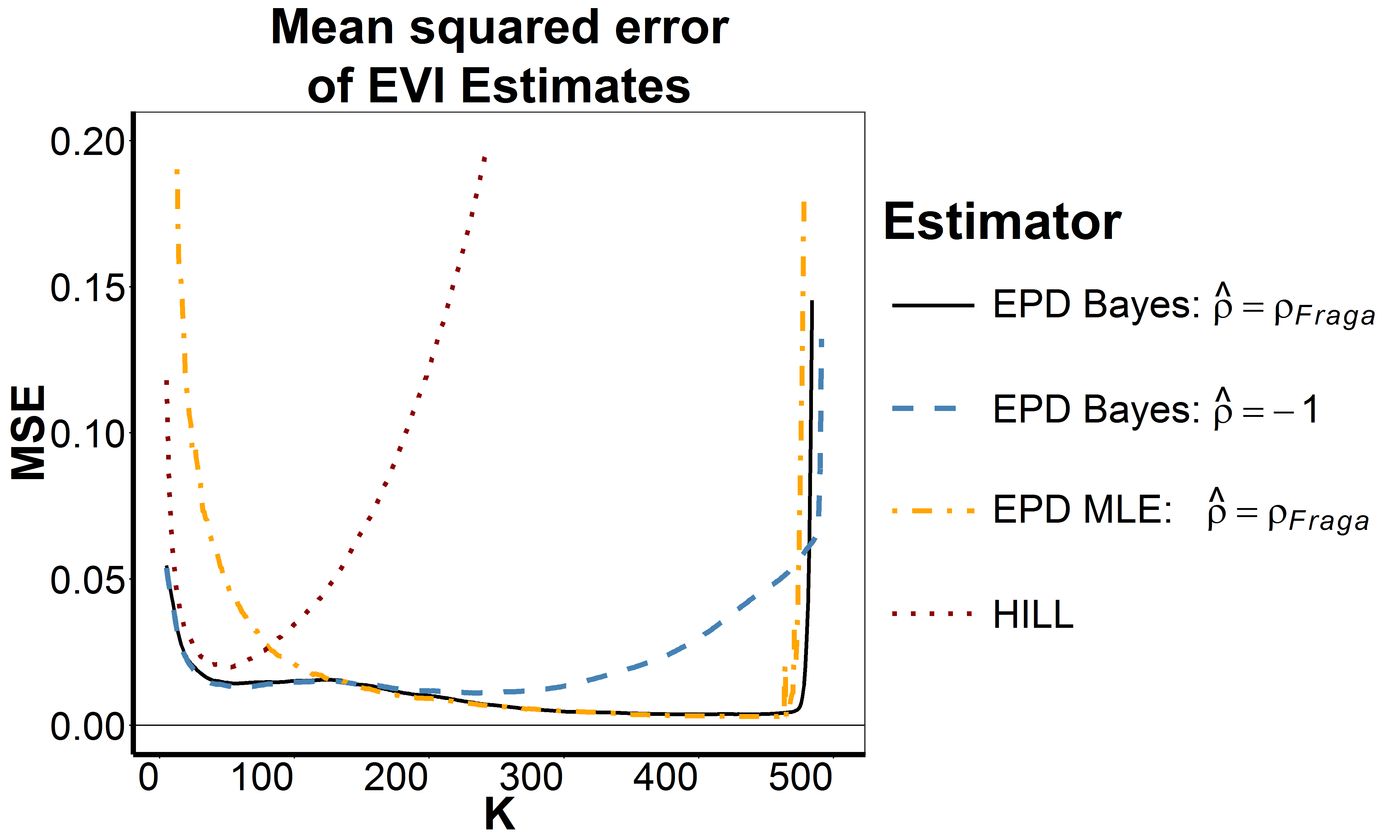
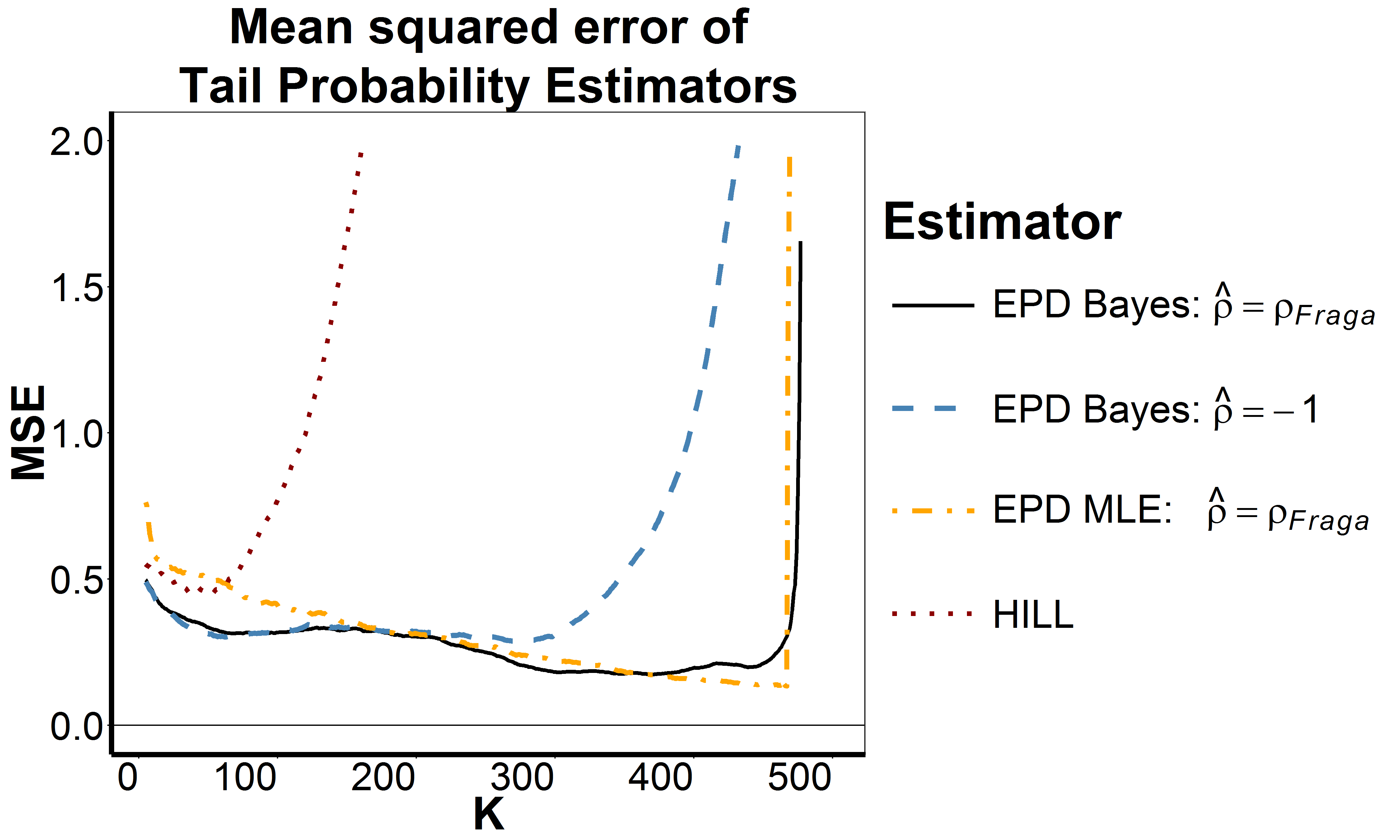
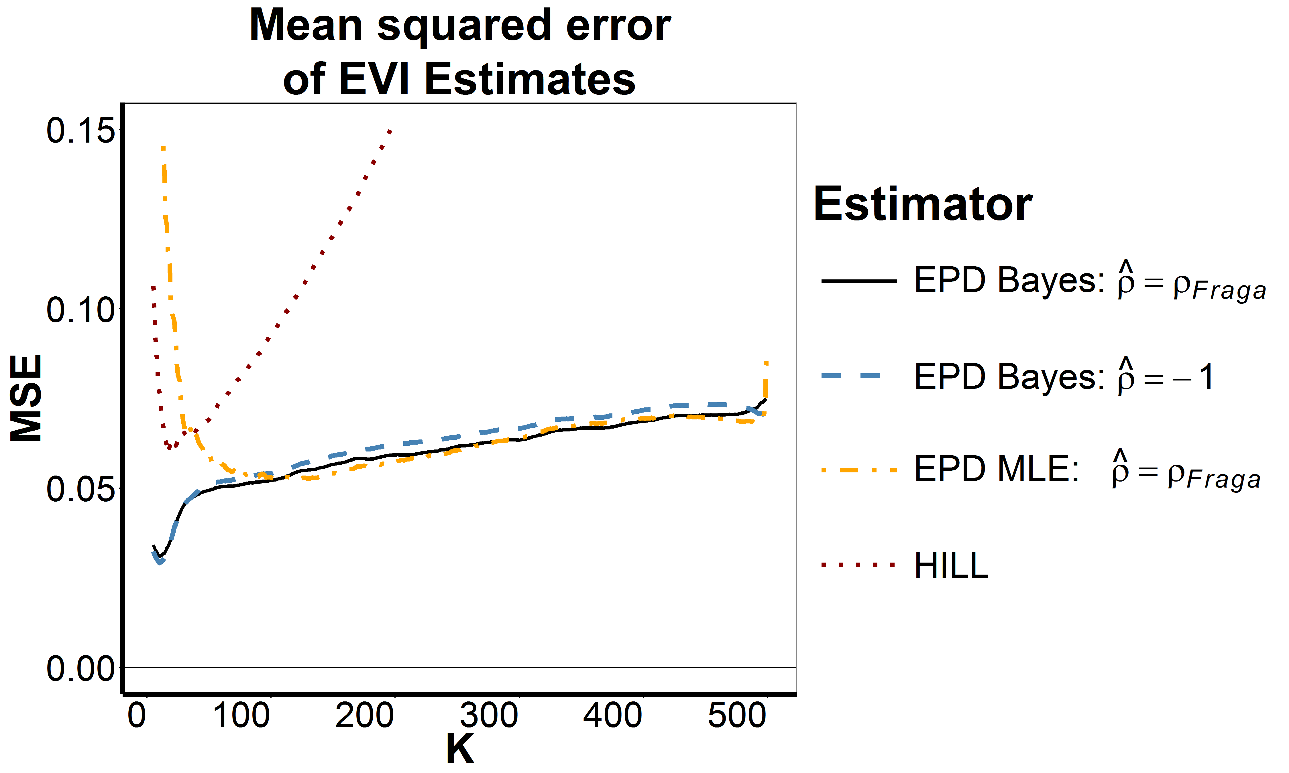
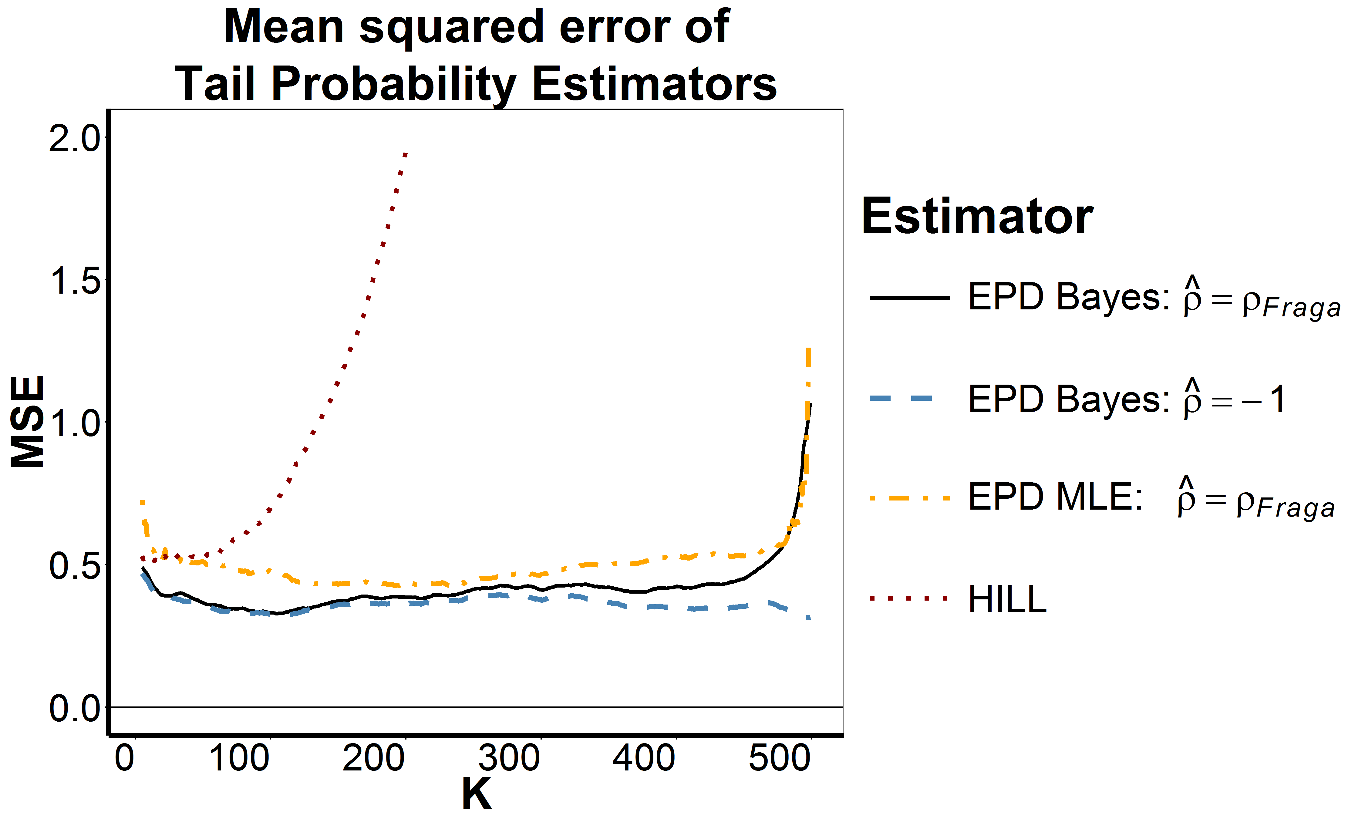
We performed a simulation study, taking 1000 repetitions of samples of size $n=500$ studying the finite sample behaviour of $\hat{\xi}^{*}_{k,n}$ and $\hat{p}^{*}_{x,k}$ with $x=Q(1-1/500)$ for different distributions, using the estimator $\hat{\rho}$ proposed by Fraga Alves et al. (2003) and the results are shown in figures 1 to 3. The bias, variance and MSE are plotted as a function of $k$. In case of the tail probability estimators we consider the relative error in the variance and MSE.

We compute the HPD using a direct approach of taking the shortest probability interval, given a $1-\alpha$ coverage based on the simulations. We do this by ordering the $m$ simulation draws and then taking the shortest interval that contains $(1-\alpha)*m$ of the draws.
The following distributions are used:

• The Fréchet distribution with $\bar{F}(x)=1-\exp(-x^{-1/\xi})$ taking $\xi=0.5$ in which case $\rho=-1$.

• The Burr distribution with $\bar{F}(x)=(1+x)^{-4/3}$ so that $\xi=0.75$ and $\rho=-0.75$.

• The loggamma distribution with $\bar{F}(x)\sim constant\times x^{-2}(\log x)^{3}$ so that $\xi=0.5$, which does not belong to the class $\mathcal{F}(\xi,\tau)$.

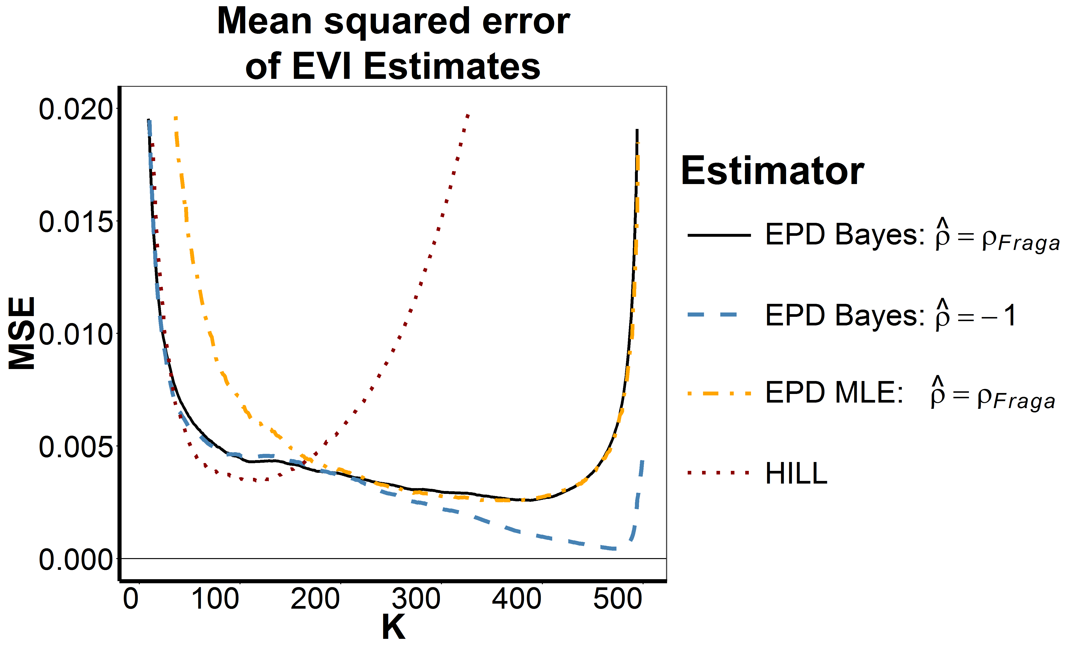
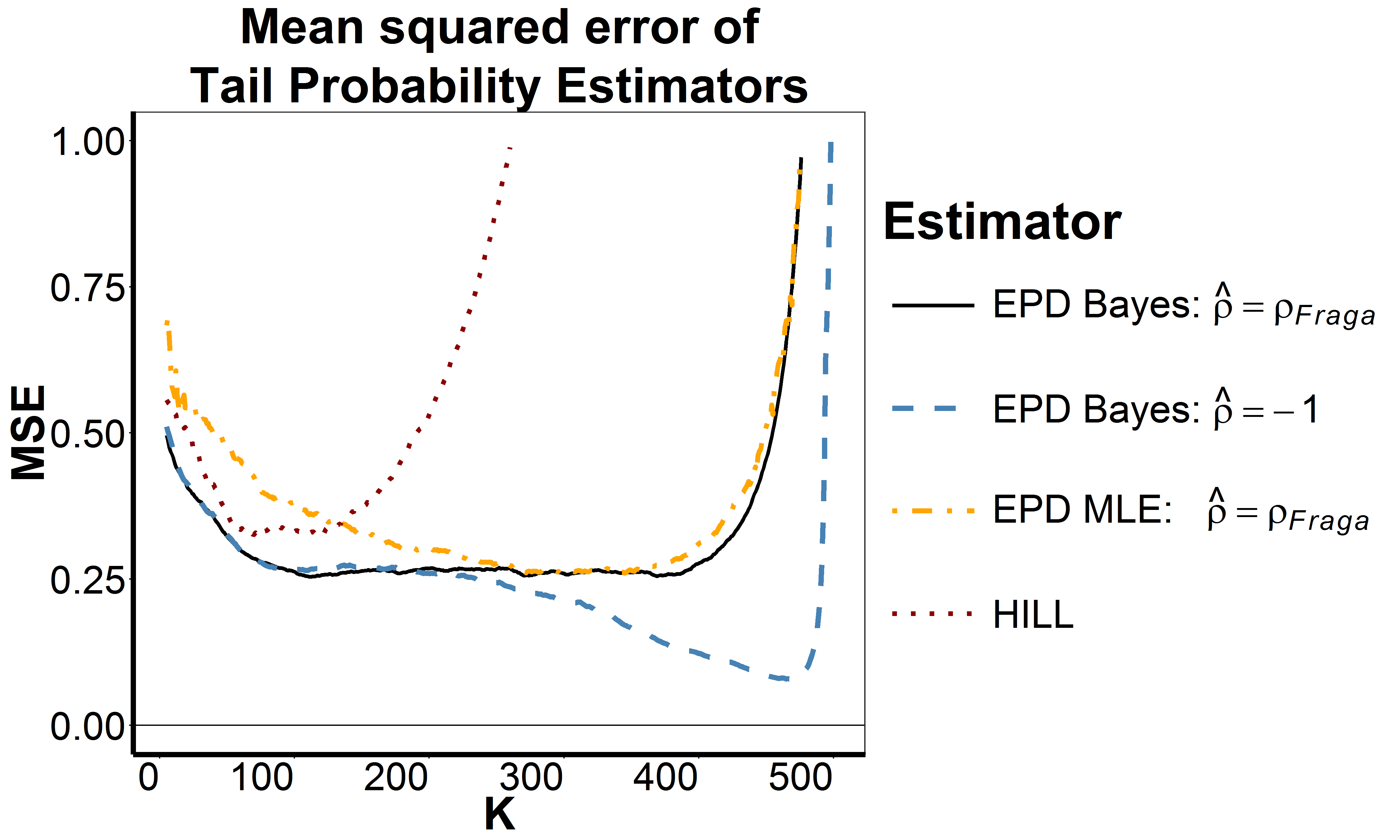
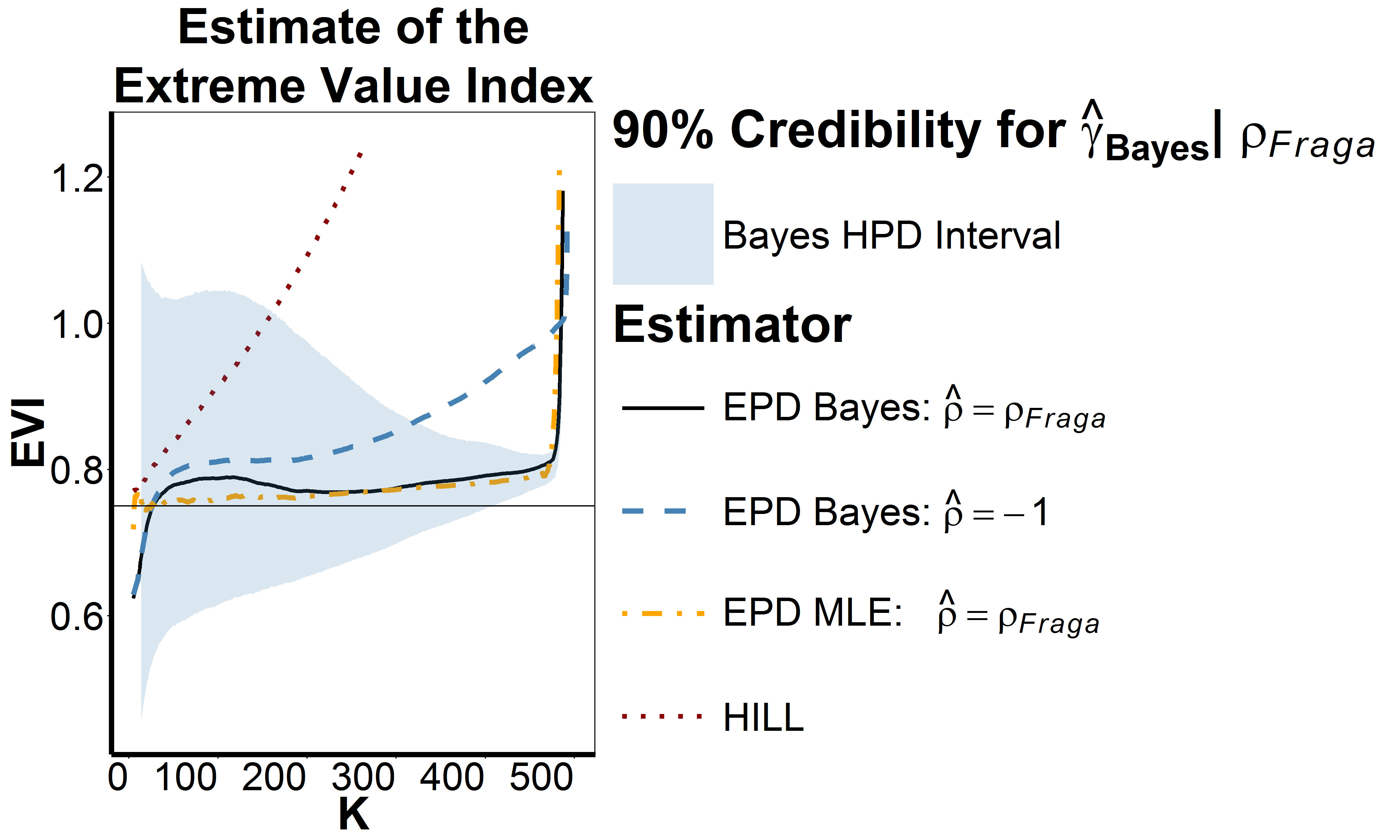
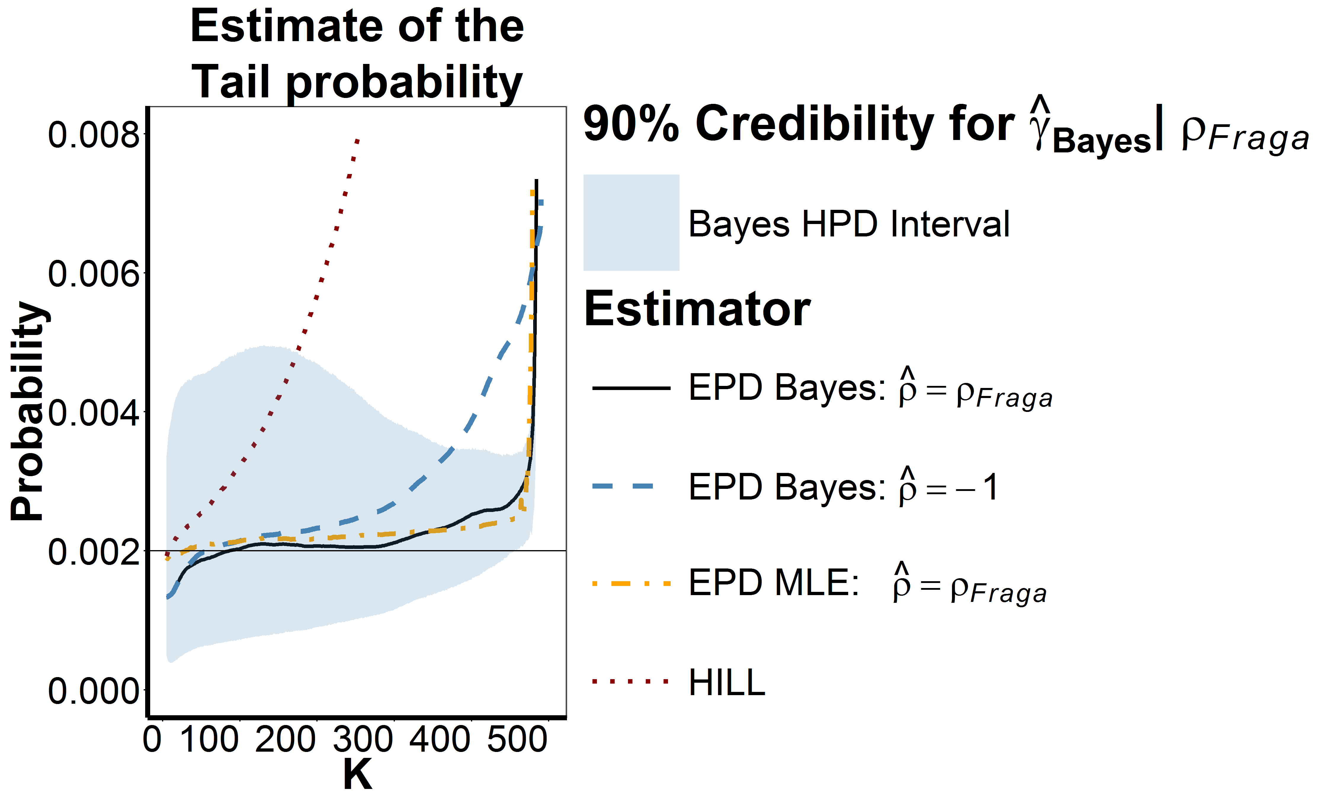
Figure 1: Bias (top), variance (middle), and mean squared error (bottom) of the estimates of $\xi$ (left) and estimates of the exceedance probability (right) using the Bayesian estimates with $\hat{\rho}=\rho_{Fraga}$ and $\rho=-1$, the classical Hill-Weissman approach, and the EPD-ML approach, in the case of a Fréchet distribution with $\xi=0.5$ and $\rho=-1$.

Figure 2: Bias (top), variance (middle), and mean squared error (bottom) of the estimates of $\xi$ (left) and estimates of the exceedance probability (right) using the Bayesian estimates with $\hat{\rho}=\rho_{Fraga}$ and $\rho=-1$, the classical Hill-Weissman approach, and the EPD-ML approach, in the case of a Burr distribution with $\xi=0.75$ and $\rho=-0.75$.

Figure 3: Bias (top), variance (middle), and mean squared error (bottom) of the estimates of $\xi$ (left) and estimates of the exceedance probability (right) using the Bayesian estimates with $\hat{\rho}=\rho_{Fraga}$ and $\rho=-1$, the classical Hill-Weissman approach, and the EPD-ML approach, in the case of a loggamma distribution with $\xi=0.5$ and $\rho=0$.

We conclude that the finite sample behaviour of the proposed estimators follows the characteristics predicted by the asymptotic analysis to a great extent. For small $k$ the Bayesian estimators $\xi_{k,n}^{*}$ and $\hat{p}^{*}_{x,k}$ show a similar behaviour as the Hill and Weissman estimators, while for larger $k$ the proposed estimators tend to follow the characteristics of the bias reduced EPD-ML estimator. The MSE of the Bayesian estimator of $P(X>x)$ is smallest, uniformly over the whole $k$ range and in all cases presented. Concerning the estimation of $\xi$, only in the Fréchet case and for small $k$ does the Hill estimator show a smaller MSE than the Bayesian estimator, while $\hat{\xi}^{*}_{k,n}$ then still shows a much smaller MSE than the EPD-ML estimator.
Also note that the version where the parameter $\rho$ is set to -1 does not differ too much from the use of the Fraga Alves et al. (2003) estimator. In case of the Fréchet distribution with $\rho=-1$, fixing this second order parameter at the correct value naturally yields some improvement in MSE, especially at large values of $k$. Similarly, fixing $\rho$ at an incorrect value, as in the case of the selected Burr distribution, yields larger MSE values at large values of $k$.
Finally the results in case of the loggamma distribution are quite good. Hence it appears that the proposed method exhibits some robustness against deviations from the underlying model.

In order to illustrate the use of the proposed method we consider the weekly negative log-returns for Barclays PLC as studied in Reynkens et al. (2015). This data is divided in two sets, before and after the 2007 financial crisis:

• Pre-Crisis: from January 1,1994 to August 7, 2007,

• Post-Crisis: from August 8,2007 to September 23, 2014.

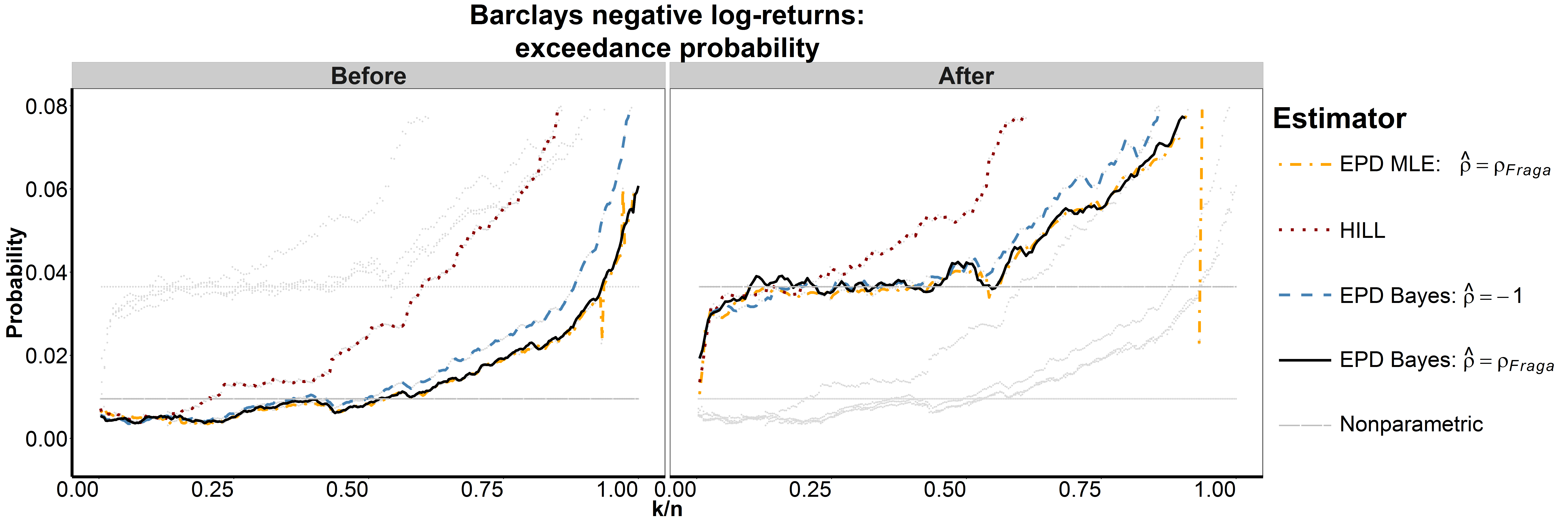
We consider the estimation of $P(X>0.18)$ in both periods. Whereas daily return data may suffer from serial dependence such as volatility clustering, such dependence is at least much weaker in weekly returns. We here use the proposed technique as a data analytic tool in order to assist the user in finding the relevant level of the estimate as a function of $k$. Up to the start of the crisis an 18% loss or higher appears to return on average once in 400 weeks (one-sided exceedance probability 0.005) based on $k/n\leq 0.25$, while as from the start of the crisis this return level decreases to close to once in 50 weeks (one-sided exceedance probability 0.04) based on $k/n\leq 0.50$.

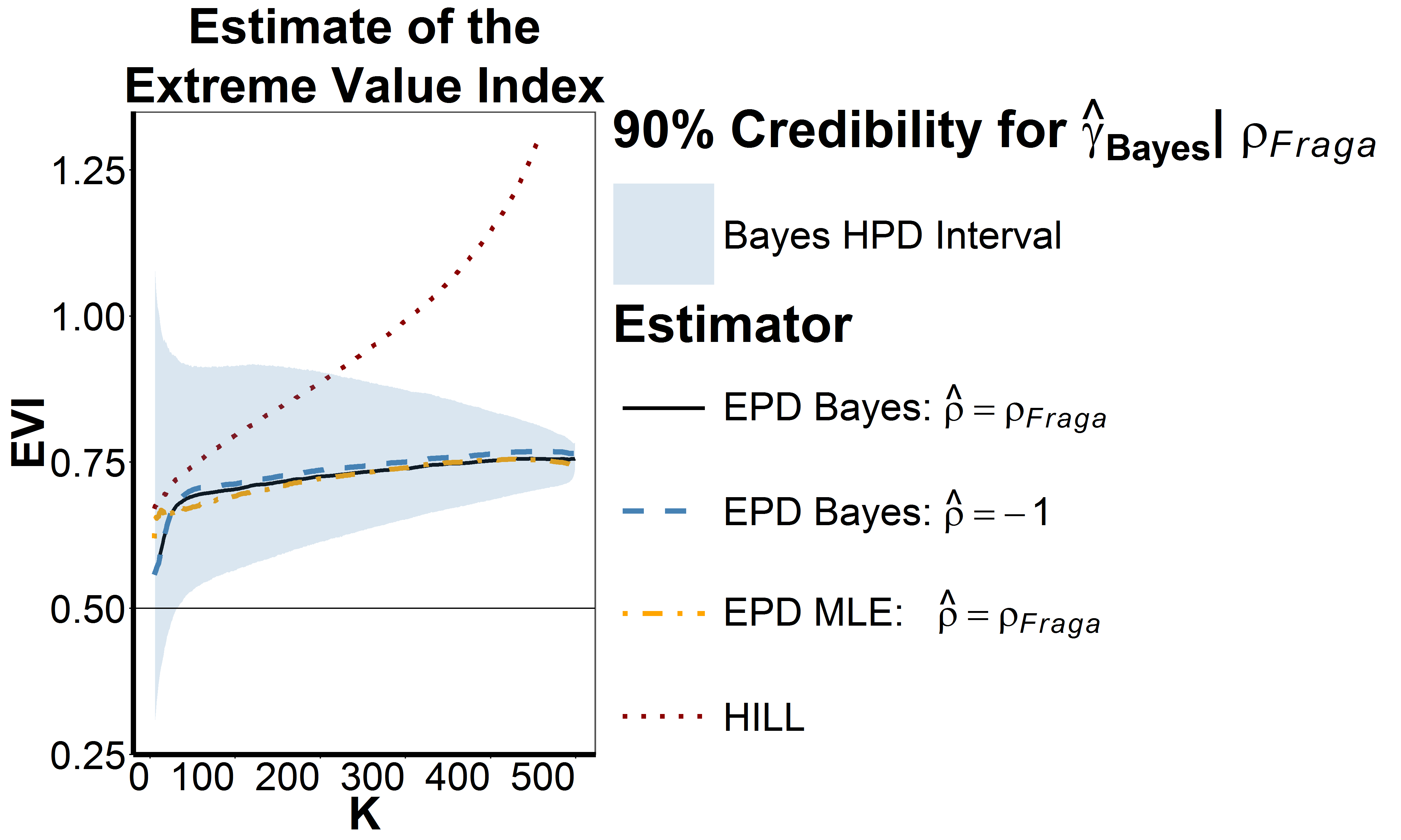
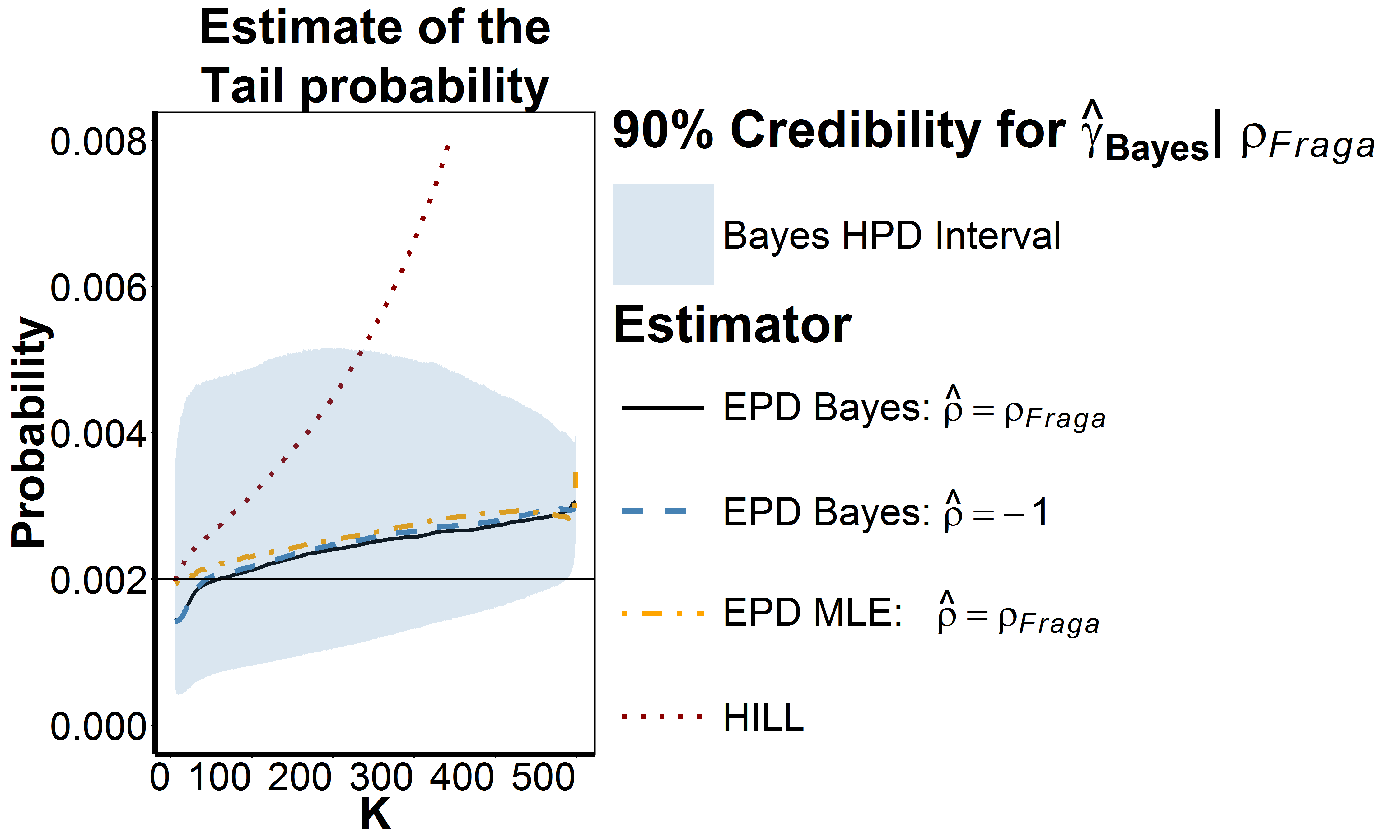
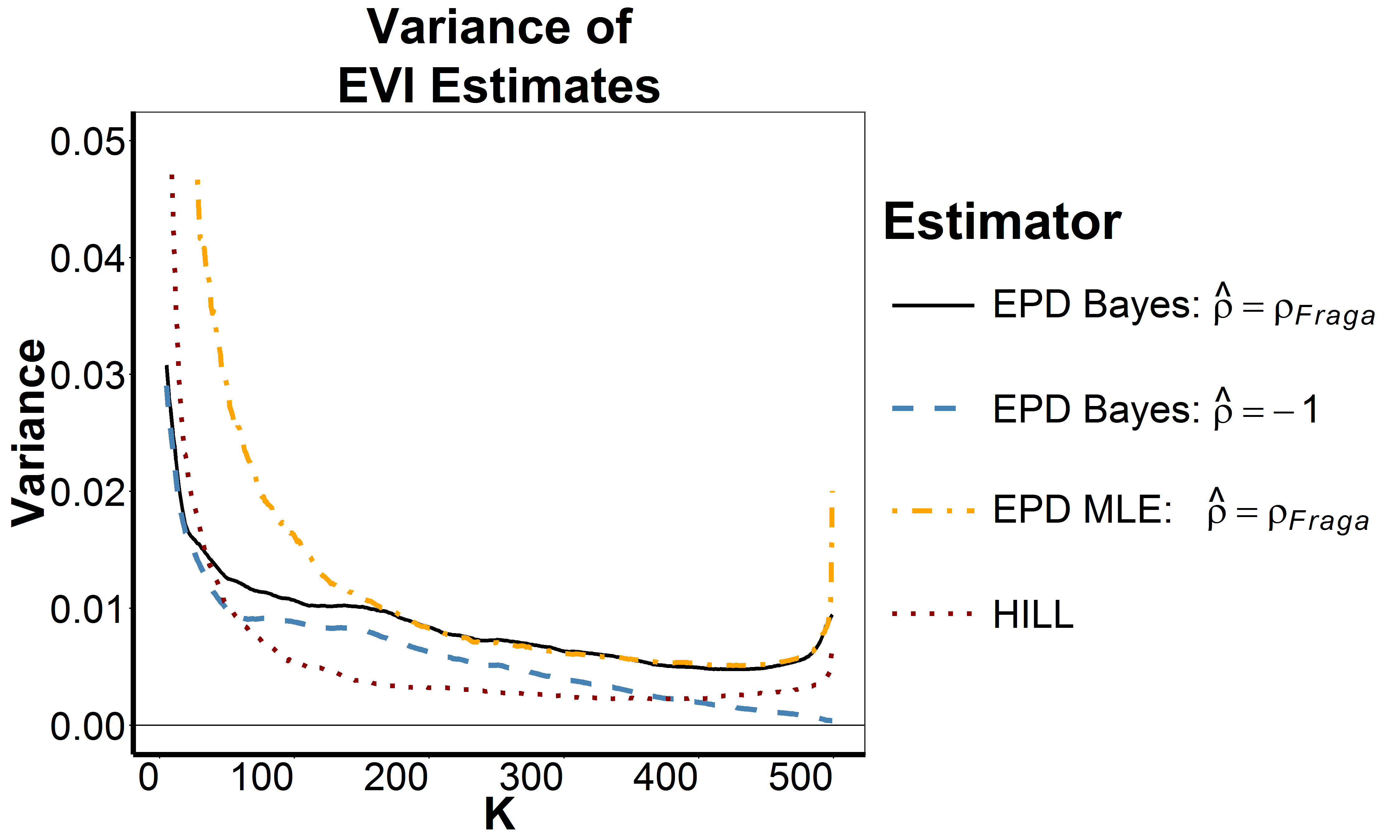
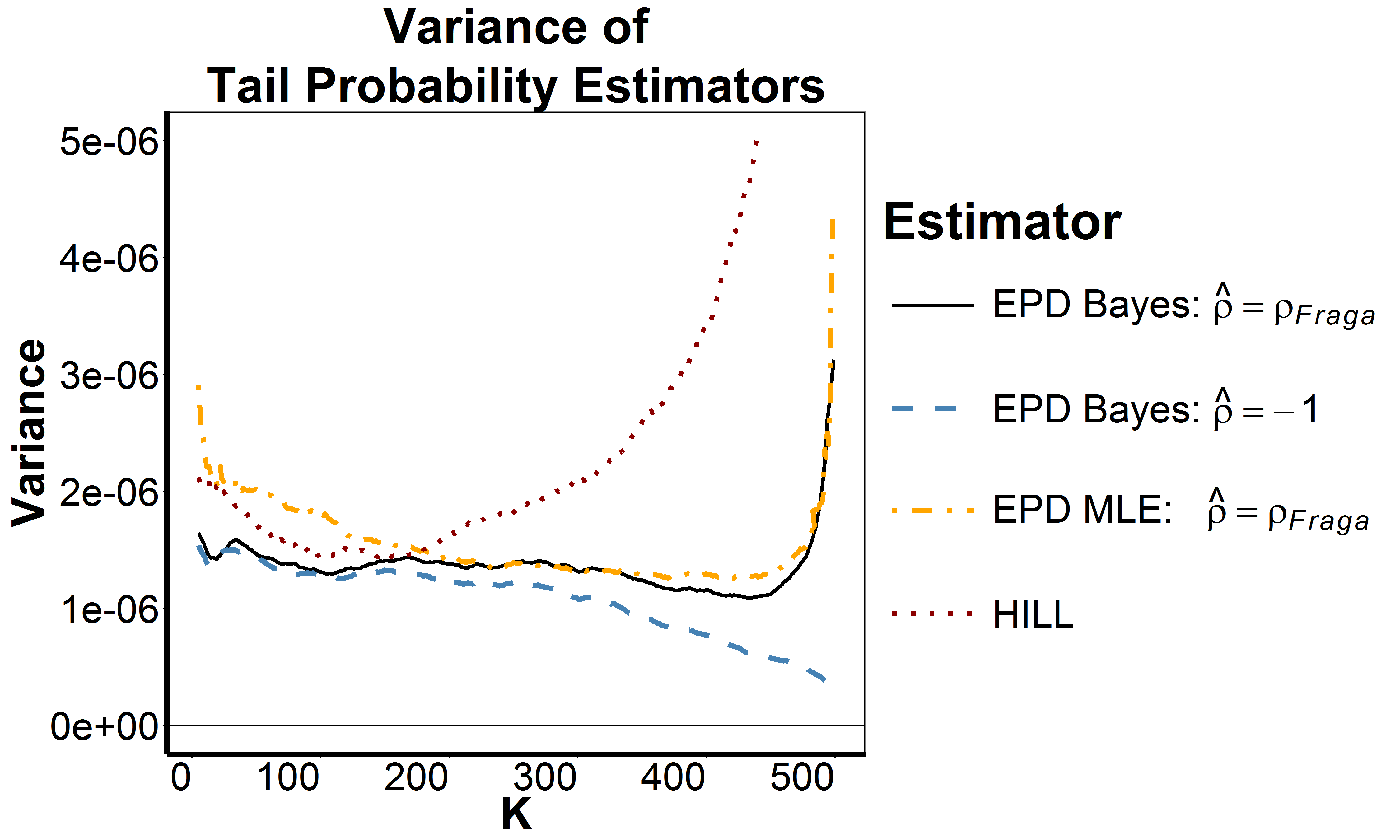
Figure 4: Estimates of the probability of exceeding 0.18 as a function of k/n for pre-crisis (left) and post-crisis (right) weekly negative log-returns of Barclays PLC

5 Conclusion

We proposed a simple adaptation to the bias reduction technique in tail estimation based on the EPD, which yields interesting MSE behaviour. In fact for larger thresholds the proposed estimators follow the behaviour of the classical Hill and Weissman estimators with small bias and minimal variance, while the new estimators are never worse than the ML estimators based on the EPD approximation. In contrast to existing minimum variance bias reduced estimators which use third order tail conditions, the conditions can be kept minimal. In fact, setting the second order parameter $\hat{\rho}$ at $-1$ still yields acceptable results.

In future work extensions of this approach to other tail estimation problems will be investigated.

Acknowledgment. The authors take pleasure in thanking S. van der Merwe for his valuable advice concerning the Bayesian implementations.

6 Appendix

Derivation of the expressions of ($\hat{\xi}_{k}^{\mathcal{B}},\hat{\delta}_{k}^{\mathcal{B}}$). First consider the asymptotic approximations of the mode-posterior estimator of $\xi$ based on maximization of (9) with (27) and (11). From (9)-(11) using expansions in $\delta\to 0$ we obtain

$${1\over k}\log\pi(\xi,\delta|{\bf y}) = -(1+{1\over k})\log\xi-{1\over k}(1+\xi)-(\frac{1}{\xi}+1){1\over k}\sum_{j=1}^{k}\log y_{j,k}$$

$$-{\delta\over 1+\xi}{1\over k}\sum_{j=1}^{k}(1-y_{j,k}^{\tau})+\delta{1\over k}\sum_{j=1}^{k}(1-(1+\tau)y_{j,k}^{\tau})$$

$$-{\delta^{2}\over 2k\sigma_{k,n}^{2}}+{\delta^{2}\over 2(1+\xi)}{1\over k}\sum_{j=1}^{k}(1-y_{j,k}^{\tau})^{2}-{\delta^{2}\over 2}{1\over k}\sum_{j=1}^{k}(1-(1+\tau)y_{j,k}^{\tau})^{2}$$

$$+O(\delta^{3})+c,$$

where $c$ is a constant only depending on $\sigma_{k,n}^{2}$ and $\tau$. Also note that ${1\over k}\sum_{j=1}^{k}\log y_{j,k}=H_{k,n}$. Then

$${\partial\over\partial\xi}{1\over k}\log\pi(\xi,\delta|{\bf y}) = -{1\over\xi}+{1\over\xi^{2}}H_{k,n}+{\delta\over\xi^{2}}{1\over k}\sum_{j=1}^{k}(1-y_{j,k}^{\tau})+O(\delta^{2})+O({1\over k}),$$

$${\partial\over\partial\delta}{1\over k}\log\pi(\xi,\delta|{\bf y}) = -{1\over\xi}\left(1-(1-\xi\tau){1\over k}\sum_{j=1}^{k}y_{j,k}^{\tau}\right)-{\delta\over k\sigma^{2}_{k,n}}$$

$$+{\delta\over\xi}\left(1-2(1-\xi\tau){1\over k}\sum_{j=1}^{k}y_{j,k}^{\tau}+(1-2\xi\tau-\xi\tau^{2}){1\over k}\sum_{j=1}^{k}y_{j,k}^{2\tau}\right)+O(\delta^{2})+O({1\over k}).$$

Derivation of Theorem. Assuming $k\sigma_{k,n}^{2}\to\mu>0$ as $k,n\to\infty$, $k/n\to 0$ and $\sqrt{k}a(n/k)\to\lambda$ we find using $E_{k,n}(s)\to 1/(1-\xi s)$ (see Theorem A.1 in Beirlant et al., 2009) that

$$D^{\mathcal{B}}_{k,n}=-{\xi\over\mu}+{\rho^{4}\over\xi(1-2\rho)(1-\rho)^{2}}+o_{p}(1).$$

Then, proceeding as in the proof of Theorem 3.1 in Beirlant et al. (2009), we obtain with $\Gamma_{k,n}=\sqrt{k}(H_{k,n}-\xi)$, $\mathbb{E}_{k,n}(s)=\sqrt{k}(E_{k,n}(s)-{1\over 1-\xi s})$ ($s<0$), that

$$\sqrt{k}\left(\hat{\xi}_{k}^{\mathcal{B}}-\xi\right) = \sqrt{k}\left(H_{k,n}-\xi-\hat{\delta}_{k}^{\mathcal{B}}{\rho\over 1-\rho}\right)$$

$$= \Gamma_{k,n}-{\rho\over 1-\rho}\sqrt{k}\hat{\delta}_{k}^{\mathcal{B}}$$

$$= \Gamma_{k,n}\left(1+{\rho^{2}\over\xi(1-\rho^{2})}{1\over(\xi/\mu)+\rho^{4}/\xi(1-2\rho)(1-\rho)^{2}}\right)$$

$$-{\rho\over(\xi/\mu)+\rho^{4}/\xi(1-2\rho)(1-\rho)^{2}}\mathbb{E}_{k,n}(\hat{\tau})+o_{p}(1)$$

$$= \Gamma_{k,n}\left(1+{\rho^{2}(1-2\rho)\over\zeta+\rho^{4}}\right)+\mathbb{E}_{k,n}(\hat{\tau})\left({(-\rho)\xi(1-2\rho)(1-\rho)^{2}\over\rho^{4}+\zeta}\right)+o_{p}(1),$$

where $\zeta=\xi^{2}(1-2\rho)(1-\rho)^{2}/\mu$. Using Theorem A.1 in Beirlant et al. (2009), (15) and (16) follow under $\sqrt{k}a(n/k)\to\lambda$.

References

• [1] Beirlant, J., Dierckx, G., Goegebeur, Y. and Matthys, G., 1999. Tail index estimation and an exponential regression model. Extremes, 2(2), pp.177-200.
• [2] Beirlant, J., Dierckx, G., Guillou, A. and Staăricaă, C., 2002. On exponential representations of log-spacings of extreme order statistics. Extremes, 5(2), pp.157-180.
• [3] Beirlant, J., Goegebeur, Y., Segers, J. and Teugels, J., 2004. Statistics of extremes: theory and applications. Wiley, Chichester.
• [4] Beirlant, J., Figueiredo, F., Gomes, M.I. and Vandewalle, B., 2008. Improved reduced-bias tail index and quantile estimators. Journal of Statistical Planning and Inference, 138(6), pp.1851-1870.
• [5] Beirlant, J., Joossens, E., Segers, J., 2009. Second-order refined peaks-over-threshold modelling for heavy-tailed distribution. Journal of Statistical Planning and Inference 139, 2800-2815.
• [6] Bingham, N.H., Goldie, C.M. and Teugels, J.L., 1987. Regular Variation. 1987. Cambridge University Press.
• [7] Caeiro, F., Gomes, M.I. and Pestana, D., 2005. Direct reduction of bias of the classical Hill estimator. Revstat, 3(2), pp.113-136.
• [8] Caeiro, F., Gomes, M.I. and Rodrigues, L.H., 2009. Reduced-bias tail index estimators under a third-order framework. Communications in Statistics—Theory and Methods, 38(7), pp.1019-1040.
• [9] Feuerverger, A. and Hall, P., 1999. Estimating a tail exponent by modelling departure from a Pareto distribution. The Annals of Statistics, 27(2), pp.760-781.
• [10] Fraga Alves, M.I., Gomes, M.I. and de Haan, L., 2003. A new class of semi-parametric estimators of the second order parameter. Portugaliae Mathematica, 60(2), pp.193-214.
• [11] Gomes, M.I., Martins, M.J. and Neves, M., 2007. Improving second order reduced bias extreme value index estimation. Revstat, 5(2), pp.177-207.
• [12] Hall, P., 1982. On some simple estimates of an exponent of regular variation. Journal of the Royal Statistical Society. Series B (Methodological), pp.37-42.
• [13] Hill, B.M., 1975. A simple general approach to inference about the tail of a distribution. The annals of statistics, 3(5), pp.1163-1174.
• [14] Lunn, D., Jackson, C., Best, N., Thomas, A. and Spiegelhalter, D., 2012. The BUGS book: A practical introduction to Bayesian analysis. CRC press.
• [15] Peng, L., 1998. Asymptotically unbiased estimators for the extreme-value index. Statistics & Probability Letters, 38(2), pp.107-115.
• [16] Reynkens, T., Beirlant, J., De Spiegeleer, J., Herrmann, K., Schoutens, W. (2015). Hunting for Black Swans in the European banking sector using extreme value analysis. 9th International EVA conference. Ann Arbor, MI, 14-19 June 2015.
• [17] Weissman, I., 1978. Estimation of parameters and large quantiles based on the k largest observations. Journal of the American Statistical Association, 73(364), pp.812-815.
6 Appendix
Derivation of the expressions of (ξ^k,δ^ksuperscriptsubscript^𝜉𝑘superscriptsubscript^𝛿𝑘\hat{\xi}_{k}^{\mathcal{B}},\hat{\delta}_{k}^{\mathcal{B}}). First consider the asymptotic approximations of the mode-posterior estimator of ξ𝜉\xi based on maximization of (9) with (27) and (11). From (9)-(11) using expansions in δ0𝛿0\delta\to 0 we obtain
1klogπ(ξ,δ|𝐲)1𝑘𝜋𝜉conditional𝛿𝐲\displaystyle{1\over k}\log\pi(\xi,\delta|{\bf y}) =\displaystyle= (1+1k)logξ1k(1+ξ)(1ξ+1)1kj=1klogyj,k11𝑘𝜉1𝑘1𝜉1𝜉11𝑘superscriptsubscript𝑗1𝑘subscript𝑦𝑗𝑘\displaystyle-(1+{1\over k})\log\xi-{1\over k}(1+\xi)-(\frac{1}{\xi}+1){1\over k}\sum_{j=1}^{k}\log y_{j,k}
δ1+ξ1kj=1k(1yj,kτ)+δ1kj=1k(1(1+τ)yj,kτ)𝛿1𝜉1𝑘superscriptsubscript𝑗1𝑘1superscriptsubscript𝑦𝑗𝑘𝜏𝛿1𝑘superscriptsubscript𝑗1𝑘11𝜏superscriptsubscript𝑦𝑗𝑘𝜏\displaystyle-{\delta\over 1+\xi}{1\over k}\sum_{j=1}^{k}(1-y_{j,k}^{\tau})+\delta{1\over k}\sum_{j=1}^{k}(1-(1+\tau)y_{j,k}^{\tau})
δ22kσk,n2+δ22(1+ξ)1kj=1k(1yj,kτ)2δ221kj=1k(1(1+τ)yj,kτ)2superscript𝛿22𝑘superscriptsubscript𝜎𝑘𝑛2superscript𝛿221𝜉1𝑘superscriptsubscript𝑗1𝑘superscript1superscriptsubscript𝑦𝑗𝑘𝜏2superscript𝛿221𝑘superscriptsubscript𝑗1𝑘superscript11𝜏superscriptsubscript𝑦𝑗𝑘𝜏2\displaystyle-{\delta^{2}\over 2k\sigma_{k,n}^{2}}+{\delta^{2}\over 2(1+\xi)}{1\over k}\sum_{j=1}^{k}(1-y_{j,k}^{\tau})^{2}-{\delta^{2}\over 2}{1\over k}\sum_{j=1}^{k}(1-(1+\tau)y_{j,k}^{\tau})^{2}
+O(δ3)+c,𝑂superscript𝛿3𝑐\displaystyle+O(\delta^{3})+c,
where c𝑐c is a constant only depending on σk,n2superscriptsubscript𝜎𝑘𝑛2\sigma_{k,n}^{2} and τ𝜏\tau. Also note that 1kj=1klogyj,k=Hk,n1𝑘superscriptsubscript𝑗1𝑘subscript𝑦𝑗𝑘subscript𝐻𝑘𝑛{1\over k}\sum_{j=1}^{k}\log y_{j,k}=H_{k,n}. Then
ξ1klogπ(ξ,δ|𝐲)𝜉1𝑘𝜋𝜉conditional𝛿𝐲\displaystyle{\partial\over\partial\xi}{1\over k}\log\pi(\xi,\delta|{\bf y}) =\displaystyle= 1ξ+1ξ2Hk,n+δξ21kj=1k(1yj,kτ)+O(δ2)+O(1k),1𝜉1superscript𝜉2subscript𝐻𝑘𝑛𝛿superscript𝜉21𝑘superscriptsubscript𝑗1𝑘1superscriptsubscript𝑦𝑗𝑘𝜏𝑂superscript𝛿2𝑂1𝑘\displaystyle-{1\over\xi}+{1\over\xi^{2}}H_{k,n}+{\delta\over\xi^{2}}{1\over k}\sum_{j=1}^{k}(1-y_{j,k}^{\tau})+O(\delta^{2})+O({1\over k}),
δ1klogπ(ξ,δ|𝐲)𝛿1𝑘𝜋𝜉conditional𝛿𝐲\displaystyle{\partial\over\partial\delta}{1\over k}\log\pi(\xi,\delta|{\bf y}) =\displaystyle= 1ξ(1(1ξτ)1kj=1kyj,kτ)δkσk,n21𝜉11𝜉𝜏1𝑘superscriptsubscript𝑗1𝑘superscriptsubscript𝑦𝑗𝑘𝜏𝛿𝑘subscriptsuperscript𝜎2𝑘𝑛\displaystyle-{1\over\xi}\left(1-(1-\xi\tau){1\over k}\sum_{j=1}^{k}y_{j,k}^{\tau}\right)-{\delta\over k\sigma^{2}_{k,n}}
+δξ(12(1ξτ)1kj=1kyj,kτ+(12ξτξτ2)1kj=1kyj,k2τ)+O(δ2)+O(1k).𝛿𝜉121𝜉𝜏1𝑘superscriptsubscript𝑗1𝑘superscriptsubscript𝑦𝑗𝑘𝜏12𝜉𝜏𝜉superscript𝜏21𝑘superscriptsubscript𝑗1𝑘superscriptsubscript𝑦𝑗𝑘2𝜏𝑂superscript𝛿2𝑂1𝑘\displaystyle+{\delta\over\xi}\left(1-2(1-\xi\tau){1\over k}\sum_{j=1}^{k}y_{j,k}^{\tau}+(1-2\xi\tau-\xi\tau^{2}){1\over k}\sum_{j=1}^{k}y_{j,k}^{2\tau}\right)+O(\delta^{2})+O({1\over k}).
Derivation of Theorem. Assuming kσk,n2μ>0𝑘superscriptsubscript𝜎𝑘𝑛2𝜇0k\sigma_{k,n}^{2}\to\mu>0 as k,n𝑘𝑛k,n\to\infty, k/n0𝑘𝑛0k/n\to 0 and ka(n/k)λ𝑘𝑎𝑛𝑘𝜆\sqrt{k}a(n/k)\to\lambda we find using Ek,n(s)1/(1ξs)subscript𝐸𝑘𝑛𝑠11𝜉𝑠E_{k,n}(s)\to 1/(1-\xi s) (see Theorem A.1 in Beirlant et al., 2009) that
Dk,n=ξμ+ρ4ξ(12ρ)(1ρ)2+op(1).subscriptsuperscript𝐷𝑘𝑛𝜉𝜇superscript𝜌4𝜉12𝜌superscript1𝜌2subscript𝑜𝑝1D^{\mathcal{B}}_{k,n}=-{\xi\over\mu}+{\rho^{4}\over\xi(1-2\rho)(1-\rho)^{2}}+o_{p}(1).