Illuminating Molecular Symmetries with Bicircular High-Order-Harmonic Generation

Abstract

We present a complete theory of bicircular high-order-harmonic emission from $N$-fold rotationally symmetric molecules. Using a rotating frame of reference we predict the complete structure of the high-order-harmonic spectra for arbitrary driving frequency ratios and show how molecular symmetries can be directly identified from the harmonic signal. Our findings reveal that a characteristic fingerprint of rotational molecular symmetries can be universally observed in the ultrafast response of molecules to strong bicircular fields.

High-order-harmonic generation (HHG) represents one of the primary gateways towards obtaining novel table-top light sources with unique properties for a wide range of applications Popmintchev et al. (2010). At the same time it holds the promise to revolutionize our understanding of fundamental dynamical processes in atoms and molecules, demonstrated for example by the ultrafast tracing of charge migration in iodoacetylene Kraus et al. (2015), as well as in condensed-matter systems, exemplified by the advent of extreme ultraviolet spectroscopy in solids Luu et al. (2015). While the generation of bright linearly polarized light through HHG is well-established Rundquist et al. (1998), efforts to expand the toolbox of ultrafast light probes towards circular and elliptical polarization have subsequently attracted great interest, motivated by the vast potential for applications in, e.g., the study of circular dichroism in chiral molecules Böwering et al. (2001) or the direct measurement of quantum phases Liu et al. (2011); Xu et al. (2012). The most promising approach, namely HHG of circularly polarized light by bicircular driving, has recently garnered much attention due to several groundbreaking experiments demonstrating tunable polarization through helicity-selective phase matching Fleischer et al. (2014); Kfir et al. (2015, 2016), the generation of isolated attosecond pulses Hickstein et al. (2015), the extension into the X-ray regime Fan et al. (2015) and even detailed three-dimensional tomography of the emitted high-order-harmonic fields Chen et al. (2016). Even though the generation of circularly polarized pulses via HHG was theoretically examined already in the 1990s Eichmann et al. (1995); Long et al. (1995); Becker et al. (1999); Milošević et al. (2000); Milošević and Becker (2000) these experimental studies reinvigorated interest also from the theoretical side particularly regarding the question of selection rules Pisanty et al. (2014); Milošević (2015) and the role of molecular and orbital symmetries Medišauskas et al. (2015); Mauger et al. (2016). Most notably, a recent article provided a detailed analysis on the correlation between symmetries and high-order-harmonic spectra in both atoms and molecules Baykusheva et al. (2016). The primary focus of most studies has been in the analysis of the simplest bicircular HHG scheme which involves a circularly polarized driver with a fundamental frequency $\omega$ and another driver with opposite circular polarization at $2\omega$. For atomic targets one observes in this setup harmonics of opposite circularly polarization at frequencies $(3n+1)\omega$ and $(3n+2)\omega$ ($n\in\mathbb{N}$) whereas no signal is observed for frequencies $3n\omega$. For molecular targets this pattern generally becomes more elaborate Mauger et al. (2016); Baykusheva et al. (2016).

In a previous work Reich and Madsen (2016) we argued that bicircular HHG can be understood by using a rotating frame of reference. In the case of a spherically symmetric target the neighboring high-order-harmonic peaks in the laboratory frame can be understood to originate from a linearly polarized harmonic in the rotating frame. This explains, e.g., the similar emission strength of those two harmonics from $s$ states in atomic targets, a fact also reported in Baykusheva et al. (2016). While the orbital symmetry hence influences the relative strength, the molecular symmetry can completely lead to the appearance and disappearance of certain peaks in the spectrum. Although the connection between dynamical symmetries and HHG selection rules has been known for a long time Averbukh et al. (1999); Ceccherini et al. (2001); Ceccherini and Bauer (2001), the imprint of the molecular symmetry for bicircular driving has only recently been discussed Mauger et al. (2016); Baykusheva et al. (2016). Still, up to this point the focus was mostly on specific driving-field configurations under particular rotational symmetries. Notably, only setups where the driving field consist of frequencies with an integer multiple have been considered. Here, we present a model using the rotating-frame picture that makes this restriction unnecessary. In fact, we show that the fingerprint of arbitrary $N$-fold rotational molecular symmetries can be found in any bicircular driving scheme with driving pulses of equal strength pointing to the possibility of ultrafast readout of molecular symmetries in, e.g., chemical reactions.

We begin by briefly reviewing the rotating-frame transformation for a field-free Hamiltonian $H_{0}$ under the influence of the electric field of two counter-rotating circularly polarized pulses with envelope $F_{0}\left(t\right)$ and frequencies $\omega,\omega^{{}^{\prime}}$ polarized in the $xy$-plane,

$$H\left(t\right) = H_{0}+F_{0}\left(t\right)[x\cos\left(\omega t\right)+y\sin\left(\omega t\right)$$ (1)

$$+x\cos(\omega^{{}^{\prime}}t)-y\sin(\omega^{{}^{\prime}}t)]\,.$$

Although we employ a single-active-electron picture it is straightforward to show that the following discussion holds even when multiple electrons are considered, see the appendix for details.

The unitary transformation $U\left(t\right)=e^{-i\alpha tL_{z}}$, with $\alpha=(\omega^{{}^{\prime}}-\omega)/2$ and $L_{z}$ the operator of angular momentum corresponding to rotation around the $z$ axis, leads to the Hamiltonian in the rotating frame

$$H^{{}^{\prime}}\left(t\right)=H_{0}^{{}^{\prime}}\left(t\right)+\alpha L_{z}+2F_{0}\left(t\right)x\cos\left(\tilde{\omega}t\right)\,,$$ (2)

where $\tilde{\omega}=(\omega+\omega^{{}^{\prime}})/2$ and $H_{0}^{{}^{\prime}}\left(t\right)=U\left(t\right)H_{0}U^{\dagger}\left(t\right)$ Reich and Madsen (2016). Equation (2) demonstrates that in a rotating frame the dynamics of two counter-rotating circularly polarized driving fields can be interpreted as a single linearly polarized driver with double the field strength at the mean frequency with an additional angular momentum term, which we call the Coriolis term, proportional to half the difference frequency. In the rotating frame the nuclei are rotating with angular frequency $\alpha$ in the $xy$-plane, indicated by the time dependence of $H_{0}^{{}^{\prime}}(t)$.

The right-circularly polarized (RCP), respectively left-circularly polarized (LCP), signal in the laboratory frame $S^{\text{lab}}\left(\Omega\right)$ is obtained via the corresponding signal in the rotating frame shifted in frequency by $\alpha$ to the left, respectively to the right, i.e., Reich and Madsen (2016)

$$S_{\text{RCP}}^{\text{lab}}\left(\Omega-\alpha\right)=S_{\text{RCP}}^{\text{rot}}\left(\Omega\right),\,\,S_{\text{LCP}}^{\text{lab}}\left(\Omega+\alpha\right)=S_{\text{LCP}}^{\text{rot}}\left(\Omega\right)\,.$$ (3)

These formulas are valid even in the absence of axial symmetry. In a non-axially symmetric setting, however, the linearly polarized driver in the rotating frame will now irradiate a rotating target. As such the simple selection rule leading to only odd multiples of the driving frequency in the rotating frame ceases to be valid.

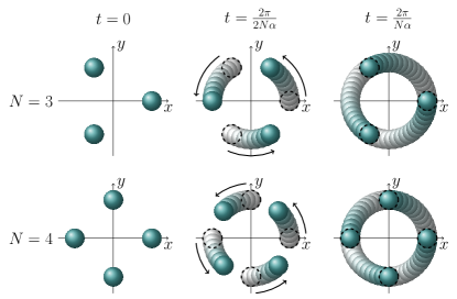
Figure 1: Illustration of nuclear rotation in the rotating frame for $N$-fold rotational symmetry with $N=3,4$. The position of the nuclei recurs after a period of $2\pi/N\alpha$, the initial position is indicated for reference by a dashed circle. At the half-point $t=2\pi/2N\alpha$ the projected potential in $x$-direction inverts for odd $N$ whereas for even $N$ the inversion symmetry is preserved for all times.

Since the bicircular driving field is polarized in the $xy$-plane the HHG process is well-described in two dimensions. Moreover, we can simplify our discussion even further by focusing on the projection of the molecular potential in $x$-direction in the rotating frame, i.e., $V\left(x,t\right)\equiv V\left(x,y=0,t\right)$. This is motivated by the fact that the driving field in the rotating frame is linearly polarized in the $x$-direction and the ground-state wave function is centered at the rotational center, i.e., $\langle y\rangle=0$. Thus, ionization events, which are the first step in HHG according to the three-step model Corkum (1993); Schafer et al. (1993); Lewenstein et al. (1994), are centered around $y=0$. Moreover, we showed in Ref. Reich and Madsen (2016) that the deflection from the Coriolis term is generally negligible even for moderately high values of $\alpha$ and only leads to a depression of the high-order-harmonic plateau but neither alters the symmetry nor the selection rules.

	$V_{0}$	actual driver	virtual driver	total	line
$N$ odd	$\left[+\right]$	$m\tilde{\omega}$, $m$ odd $\left[-\right]$	none $\left[+\right]$	$\left[-\right]$	main
	$\left[+\right]$	$m\tilde{\omega}$, $m$ odd $\left[-\right]$	$\pm N\alpha$ $\left[-\right]$	$\left[+\right]$	✗
	$\left[+\right]$	$m\tilde{\omega}$, $m$ odd $\left[-\right]$	$\pm 2N\alpha$ $\left[+\right]$	$\left[-\right]$	$2^{\text{nd}}$ side
	$\left[+\right]$	$\bar{m}\tilde{\omega}$, $\bar{m}$ even $\left[+\right]$	none $\left[+\right]$	$\left[+\right]$	✗
	$\left[+\right]$	$\bar{m}\tilde{\omega}$, $\bar{m}$ even $\left[+\right]$	$\pm N\alpha$ $\left[-\right]$	$\left[-\right]$	$1^{\text{st}}$ side
	$\left[+\right]$	$\bar{m}\tilde{\omega}$, $\bar{m}$ even $\left[+\right]$	$\pm 2N\alpha$ $\left[+\right]$	$\left[+\right]$	✗
$N$ even	$\left[+\right]$	$m\tilde{\omega}$, $m$ odd $\left[-\right]$	none $\left[+\right]$	$\left[-\right]$	main
	$\left[+\right]$	$m\tilde{\omega}$, $m$ odd $\left[-\right]$	$\pm N\alpha$ $\left[+\right]$	$\left[-\right]$	$1^{\text{st}}$ side
	$\left[+\right]$	$m\tilde{\omega}$, $m$ odd $\left[-\right]$	$\pm 2N\alpha$ $\left[+\right]$	$\left[-\right]$	$2^{\text{nd}}$ side
	$\left[+\right]$	$\bar{m}\tilde{\omega}$, $\bar{m}$ even $\left[+\right]$	none $\left[+\right]$	$\left[+\right]$	✗
	$\left[+\right]$	$\bar{m}\tilde{\omega}$, $\bar{m}$ even $\left[+\right]$	$\pm N\alpha$ $\left[+\right]$	$\left[+\right]$	✗
	$\left[+\right]$	$\bar{m}\tilde{\omega}$, $\bar{m}$ even $\left[+\right]$	$\pm 2N\alpha$ $\left[+\right]$	$\left[+\right]$	✗

Table 1: Possible combinations of actual and virtual driving (as defined in the main text) with corresponding parity indicated by $[+]$ (even) and $[-]$ (odd). The total parity is the product of the constituents’ parities. Signals with even total parity are forbidden (indicated by ✗). Signals with high order $k$ in the virtual driving, cf. Eq. (6), are generally expected to be less pronounced.

		main	$1^{\text{st}}$ side (I)	$1^{\text{st}}$ side (II)	$2^{\text{nd}}$ side (I)	$2^{\text{nd}}$ side (II)
general case, even $N$	RCP	$m\tilde{\omega}-\alpha$	$m\tilde{\omega}+\left(N-1\right)\alpha$	$m\tilde{\omega}-\left(N+1\right)\alpha$	$m\tilde{\omega}+\left(2N-1\right)\alpha$	$m\tilde{\omega}-\left(2N+1\right)\alpha$
($m\in\mathbb{N}$ odd)	LCP	$m\tilde{\omega}+\alpha$	$m\tilde{\omega}+\left(N+1\right)\alpha$	$m\tilde{\omega}-\left(N-1\right)\alpha$	$m\tilde{\omega}+\left(2N+1\right)\alpha$	$m\tilde{\omega}-\left(2N-1\right)\alpha$
general case, odd $N$	RCP	$m\tilde{\omega}-\alpha$	$\bar{m}\tilde{\omega}+\left(N-1\right)\alpha$	$\bar{m}\tilde{\omega}-\left(N+1\right)\alpha$	$m\tilde{\omega}+\left(2N-1\right)\alpha$	$m\tilde{\omega}-\left(2N+1\right)\alpha$
($m\in\mathbb{N}$ odd, $\bar{m}\in\mathbb{Z}$ even)	LCP	$m\tilde{\omega}+\alpha$	$\bar{m}\tilde{\omega}+\left(N+1\right)\alpha$	$\bar{m}\tilde{\omega}-\left(N-1\right)\alpha$	$m\tilde{\omega}+\left(2N+1\right)\alpha$	$m\tilde{\omega}-\left(2N-1\right)\alpha$
$N=3$, $\tilde{\omega}=\frac{3}{2}\omega$, $\alpha=\frac{1}{3}\tilde{\omega}=\frac{1}{2}\omega$	RCP	$3n\omega+\omega$	$3n\omega+\omega$	$3n\omega+\omega$	$3n\omega+\omega$	$3n\omega+\omega$
($n\in\mathbb{N}$)	LCP	$3n\omega+2\omega$	$3n\omega+2\omega$	$3n\omega+2\omega$	$3n\omega+2\omega$	$3n\omega+2\omega$
$N=3$, $\tilde{\omega}=2\omega$, $\alpha=\frac{1}{2}\tilde{\omega}=\omega$	RCP	$4n\omega+\omega$	$4n\omega+2\omega$	$4n\omega$	$4n\omega+3\omega$	$4n\omega+3\omega$
($n\in\mathbb{N}$)	LCP	$4n\omega+3\omega$	$4n\omega$	$4n\omega+2\omega$	$4n\omega+\omega$	$4n\omega+\omega$

Table 2: Predicted leading-order signals in general and for the two particular setups analyzed in Ref. Mauger et al. (2016) in the laboratory frame. In the latter case we report the lines for easier comparison in terms of the frequency $\omega$ of the RCP driver, cf. Eq. (1). The two branches of the side lines, indicated by I and II in the table header, correspond to absorption, respectively emission, from the virtual driver, cf. the $\pm$ sign in Table 1. Note the opposite convention for RCP and LCP compared to Ref. Mauger et al. (2016).

Figure 2: HHG signal obtained by numerical simulations for $N=3$ (top) and $N=4$ (bottom) (left for RCP signal and right for LCP signal). The circles indicate the expected position of the main line, the squares and triangles indicate the primary, respectively, secondary, side line.

At the center of our model lies the observation that the molecular potential in the rotating frame inherits a dynamical symmetry if a static rotational symmetry in the laboratory frame is present,

$$V\left(x,t\right)=V\left(x,t+\frac{2\pi}{N\alpha}\right)\,.$$ (4)

We choose $t=0$ such that $V\left(x,t\right)=V\left(x,-t\right)$, i.e., at time zero the potential is symmetric with respect to reflection on the $x$-axis, cf. Fig. 1. This allows to express the potential in a Fourier series as follows,

$$V\left(x,t\right)=V_{0}\left(x\right)+\sum_{k}V_{k}\left(x\right)\cos\left(Nk\alpha t\right)\,.$$ (5)

At this point it becomes important to distinguish between even and odd $N$. For even $N$ one observes that $V\left(x,t\right)=V\left(-x,t\right)\forall t$ for the projected potential in $x$-direction. This allows to conclude that in Eq. (5) for even $N$ all $V_{k}\left(x\right)$ are even, too. For odd $N$ we instead have the relation $V\left(x,t\right)=V\left(-x,t+\frac{2\pi}{2N\alpha}\right)$ since after half a period the potential inverts in the $x$-direction, cf. Fig. 1, and inserting this relation in Eq. (5) leads to

$$V_{0}\left(x\right)+\sum_{k}V_{k}\left(x\right)\cos\left(Nk\alpha t\right)$$

$$= V_{0}\left(-x\right)+\sum_{k}\left(-1\right)^{k}V_{k}\left(-x\right)\cos\left(Nk\alpha t\right)\,.$$

Evidently, $V_{k}\left(x\right)$ is even for even $k$ (including $k=0$) whereas it is odd for odd $k$. The Hamiltonian in the rotating frame thus reads

$$H^{{}^{\prime}}\left(t\right) = T+V_{0}\left(x\right)+\alpha L_{z}+2F_{0}\left(t\right)x\cos\left(\tilde{\omega}t\right)$$ (6)

$$+\sum_{k}V_{k}\left(x\right)\cos\left(Nk\alpha t\right)\,,$$

with $T$ denoting the kinetic energy operator and $V_{0}\left(x\right)$ representing the even time-averaged part of the potential. The form of Eq. (6) allows to interpret the time-dependence of the molecular potential in the rotating frame as additional driving fields with frequencies $Nk\alpha$ that couple spatially via the coefficient $V_{k}\left(x\right)$. We call these fields “virtual” driving fields since they appear due to the transformation to the rotating frame and the resulting rotation of the nuclei therein. This is in contrast to the “actual” driving field which is a consequence from the bicircular driving in the laboratory frame. The virtual driving field has perturbative character since its strength is related to the strength of the Coulomb potential. Specifically, when the electron gathers its energy in the continuum, particularly for higher harmonics with corresponding long excursions from the ionic core, the effect of the virtual driving is decreased with distance in contrast to the actual driving whose force on the electron is independent on the distance.

Harmonic emission is associated with the dipolar response by the driven system. In all cases $V_{0}(x)$ is even such that the combined parity of driving by the actual driver and the virtual driver needs to be odd to obtain a dipolar radiation signal, cf. Table 1. In a photon picture, for even $N$ this is only possible if an odd number of photons is absorbed by the actual driver since the virtual driver is always even so it cannot create any “oddness”. This includes the case of no participation of the virtual driver leading to the main line ($k=0$) at $m\tilde{\omega}$ for odd $m$ as well as all side lines at $m\tilde{\omega}\pm Nk\alpha$ for odd $m$ and arbitrary $k>0$. For odd $N$ there are two possibilities: If an odd number of photons is absorbed from the actual driver then the virtual driver needs to make an even contribution. This includes no contribution at all, creating the main line $m\tilde{\omega}$, and the leading even order at frequencies $\pm 2N\alpha$, which appears as a secondary side line ($k=2$) at $m\tilde{\omega}+2N\alpha$ for odd $m$. However, the primary side line ($k=1$) can be found at $\bar{m}\tilde{\omega}\pm N\alpha$ for even $\bar{m}$ since it originates from the combination of an even number of photons absorbed from the actual driver and the leading odd virtual driving at frequency $\pm N\alpha$.

Due to the comparatively small impact of the Coriolis term the emitted harmonics in the rotating frame are well-approximated as linearly polarized Reich and Madsen (2016). Thus, by Eqs. (3), they contribute roughly equally to the right- and left-circularly polarized signals in the laboratory frame. The position of the main as well as the first two side lines in the general case are shown at the top of Table 2.

It is instructive to discuss a particular example following from these general predictions. To this end we consider a three-fold molecular symmetry under the driving field configurations $\omega^{{}^{\prime}}=2\omega$ and $\omega^{{}^{\prime}}=3\omega$. The lower part of Table 2 summarizes the expected main and side lines in these two settings according to our model, expressed in terms of multiples of the fundamental driving frequency $\omega$. The polarization of particular peaks in the HHG spectrum is determined by the superposition of the contribution from the main and side lines. For $\omega^{{}^{\prime}}=2\omega$ all main and side lines with a given circular polarization coincide leading to alternating left- and right-circular polarization (RCP at $(3n+1)\omega$ and LCP at $(3n+2)\omega$, $n\in\mathbb{N}$). Conversely, for $\omega^{{}^{\prime}}=3\omega$ there exist secondary side line contributions with opposite polarization compared to the main lines at $(4n+1)\omega$ and $(4n+3)\omega$. Furthermore, there is both a left- and a right-circular contribution on the level of a first side line at $4n\omega$ and $(4n+2)\omega$. In the former case we expect the total signal to be predominantly circularly polarized since the secondary side lines are expected to be much weaker than the main line. For the latter case the superposition between opposite circular polarization occurs for side lines of the same order, hence we expect that the superposition will be close to linearly polarized. These predictions are in perfect accordance with the theoretical analysis and numerics shown in Ref. Mauger et al. (2016). We note, however, that in some settings superpositions between, e.g., main and primary side lines may occur and a precise prediction on the resulting polarization of the total signal would require a more in-depth analysis.

To illustrate our model’s high degree of predictability for general bicircular driving schemes we performed numerical simulations of the two-dimensional time-dependent Schrödinger equation using a single-active electron approximation on a set of model molecules which obey a discrete $N$-fold rotational symmetry in the $xy$-plane. They are described by a potential

$$V=\sum_{p=0}^{N-1}\frac{-Q/N}{\sqrt{\left[x-R\cos\left(\frac{2\pi p}{N}\right)\right]^{2}+\left[y-R\sin\left(\frac{2\pi p}{N}\right)\right]^{2}+a}}\,,$$

which represents a set of $N$ atomic cores at a distance $R$ from the origin evenly distributed at polar angles $\frac{2\pi}{N}$. We employ a smoothening parameter $a$ for all cores and smear out a total charge $Q$ homogeneously among them. Our calculations used the following parameter values (atomic units used throughout): $Q=2$, $R=4.01$, $a=0.251$, the driving laser field is given by a trapezoidally shaped bicircular driver with $T_{\text{ramp}}=250$ and $T_{\text{plateau}}=1500$ as well as $F_{0}=0.04$ and $\tilde{\omega}=0.0876$.

Figure 2 shows HHG spectra in the laboratory frame of RCP and LCP emission for the three-fold, respectively four-fold, cases. Evidently, the fingerprint of the corresponding molecular symmetries is well-pronounced and can be observed for all values of $\alpha$. The strong difference between odd and even $N$ is clearly revealed with the primary side lines originating at $\alpha=0$ for even multiples of $\tilde{\omega}$ for odd $N$, cf. the top panels of Fig. 2, whereas for even $N$ all main and side lines originate at odd multiples of $\tilde{\omega}$, cf. the bottom panels in Fig. 2. Generally speaking the primary side lines serve as the fundamental fingerprint of the $N$-fold rotational symmetry: While the position of the main lines is independent of $N$, the slope of the primary side lines is directly related to $N$, cf. Table 2. While the fingerprint of secondary and higher-order side lines is also characteristic for the underlying rotational symmetry their signal strength is suppressed since these lines originate from high-order contribution from the perturbative virtual driving in our model corresponding to larger values for $k$ in Eq. (6). Lastly, we note that the observation of a clear fingerprint requires that the frequencies corresponding to virtual driving are Fourier-resolved by the length of the driving field which necessitates the use of longer driving fields for smaller values of $\alpha$.

We finally emphasize that our analysis encompasses the cases of continuous symmetry (i.e. an axially symmetric target) and no symmetry. Continuous symmetry is formally equivalent to $N\rightarrow\infty$ and we therefore predict only the main line to be present in the HHG $\alpha$-scans since the slope of the side lines becomes infinite. This is consistent with, the results of Ref. Reich and Madsen (2016) where an axially symmetric atomic target was considered. In the absence of symmetry we expect that $N=1$, i.e., the potential only recurs after a full revolution in the rotating frame.

In conclusion, we have developed a model for bicircular HHG in the presence of rotational molecular symmetry that explains all principal characteristics of the observed high-order-harmonic emission. Our numerical simulations show that the resulting spectral fingerprint is well-pronounced and can be used as a reliable indicator of the presence or absence of symmetry for arbitrary driving frequencies. These findings enable the extraction of constructive tomographic information from high-order-harmonic spectra regarding molecular symmetries and can be employed to track symmetry forming and symmetry breaking on ultrafast timescales.

Appendix A Appendix: Generalization to Many-Electron Case

We show that all predictions from the main text remain valid when moving to the many-electron case. Our new starting point is the many-electron Hamiltonian

$$\tilde{H}\left(t\right) = \tilde{H}_{0}+F_{0}\left(t\right)\left(X\cos\left(\omega_{1}t\right)+Y\sin\left(\omega_{1}t\right)\right.$$

$$\left.+X\cos\left(\omega_{2}t\right)-Y\sin\left(\omega_{2}t\right)\right)\,,$$

where $\tilde{H}_{0}$ is the field-free Hamiltonian and $X=\sum_{i}x_{i}$ and $Y=\sum_{i}y_{i}$ are the sum over the Cartesian coordinates $x_{i},y_{i}$ of the $i$-th electron. The rotating-frame transformation is now performed with respect to all electrons, i.e.,

$$\tilde{U}\left(t\right)=e^{-i\alpha tL_{z}}\,,$$

with $L_{z}=\sum_{i}L_{z}^{\left(i\right)}=\sum_{i}\left[x_{i}p_{y}^{\left(i\right)}-y_{i}p_{x}^{\left(i\right)}\right]$ and $p_{x}^{(i)},p_{y}^{(i)}$ the Cartesian momenta of the $i$-th electron. Note that the operator $L_{z}$ without superscript corresponds to the total angular momentum of all electrons whereas the angular momenta of the individual electrons are indicated by $L^{(i)}_{z}$. Since all operators corresponding to different electrons commute we can also write this as

$$\tilde{U}\left(t\right)=\prod_{i}e^{-i\alpha tL_{z}^{\left(i\right)}}\,,$$ (7)

where the ordering in the product is arbitrary.

The Hamiltonian $\tilde{H}_{0}$ can be split now into one-particle (kinetic energy and electron-nuclei interactions) and two-particle (electron-electron interactions) contributions. The one-particle contributions transform exactly as discussed in the main text since only the factor in Eq. (7) corresponding to the specific electron at hand plays a role - this argument also extends to the operators $X$ and $Y$ in the bicircular driving. Furthermore the two-particle contributions are invariant since the rotation induced by the unitary transformation leaves all distances and angles between the electrons invariant. As a consequence we arrive at the rotated-frame Hamiltonian for the many-electron case,

$$\tilde{H}^{{}^{\prime}}\left(t\right)=\tilde{H}_{0}^{{}^{\prime}}\left(t\right)+\alpha L_{z}+2F_{0}\left(t\right)X\cos\left(\tilde{\omega}t\right)\,,$$

with $\tilde{H}_{0}^{{}^{\prime}}\left(t\right)=\tilde{H}_{0}\left(\left\{x_{i}\left(t\right),y_{i}\left(t\right),z_{i}\right\}\right)$, $x_{i}\left(t\right)=x_{i}\cos\left(\alpha t\right)+y_{i}\sin\left(\alpha t\right)$, and $y_{i}\left(t\right)=y_{i}\cos\left(\alpha t\right)-x_{i}\sin\left(\alpha t\right)$. This is completely analogous to the single-electron case.

Most notably, we can still define the projected potential in the rotating frame as the sum of the contributions by the individual electrons,

$$\tilde{V}\left(\left\{x_{i}\right\},t\right)=\sum_{i}V_{i}\left(x_{i},t\right)\,,$$

which follows the same symmetries as the individual contributions,

$$V_{i}\left(x_{i},t\right) = V_{i}\left(x_{i},t+\frac{2\pi}{N\alpha}\right)$$

$$\Longrightarrow\tilde{V}\left(\left\{x_{i}\right\},t\right) = \tilde{V}\left(\left\{x_{i}\right\},t+\frac{2\pi}{N\alpha}\right)\,.$$

From this point we can follow the same steps presented in the main text for a single electron and arrive at the Fourier-expanded Hamiltonian in the rotating frame for the many-electron case

$$\tilde{H}^{{}^{\prime}}\left(t\right) = \tilde{T}+V_{ee}+\sum_{i}V_{0}^{\left(i\right)}\left(x\right)+\alpha L_{z}$$

$$+2F_{0}(t)X\left(t\right)\cos\left(\tilde{\omega}t\right)+\sum_{i,k}V_{k}^{\left(i\right)}\left(x_{i}\right)\cos\left(Nk\alpha t\right)\,,$$

where the $V_{k}^{\left(i\right)}$ obey the same symmetries as in the main text for all $i$ and $V_{ee}$ contains the electron-electron interaction which is of even parity since the potential energy of all electrons is invariant under any spatial transformation. In particular, it does not depend on the molecular symmetry at all. At this point it becomes clear that all symmetry arguments with respect to the high-harmonic spectra as well as the appearance of main and side lines remain completely intact even in a many-electron description.

References

- Popmintchev et al. (2010) T. Popmintchev, M.-C. Chen, P. Arpin, M. M. Murnane, and H. C. Kapteyn, “The attosecond nonlinear optics of bright coherent x-ray generation”, Nature Photon. 4, 822–832 (2010).
- Kraus et al. (2015) P. M. Kraus, B. Mignolet, D. Baykusheva, A. Rupenyan, L. Horný, E. F. Penka, G. Grassi, O. I. Tolstikhin, J. Schneider, F. Jensen, L. B. Madsen, A. D. Bandrauk, F. Remacle, and H. J. Wörner, “Measurement and laser control of attosecond charge migration in ionized iodoacetylene”, Science 350, 790–795 (2015).
- Luu et al. (2015) T. T. Luu, M. Garg, S. Yu. Kruchinin, A. Moulet, M. Th. Hassan, and E. Goulielmakis, “Extreme ultraviolet high-harmonic spectroscopy of solids,” Nature 521, 498–502 (2015).
- Rundquist et al. (1998) A. Rundquist, Charles G. Durfee, Z. Chang, C. Herne, S. Backus, M. M. Murnane, and H. C. Kapteyn, “Phase-matched generation of coherent soft x-rays”, Science 280, 1412–1415 (1998).
- Böwering et al. (2001) N. Böwering, T. Lischke, B. Schmidtke, N. Müller, T. Khalil, and U. Heinzmann, “Asymmetry in photoelectron emission from chiral molecules induced by circularly polarized light”, Phys. Rev. Lett. 86, 1187–1190 (2001).
- Liu et al. (2011) Y. Liu, G. Bian, T. Miller, and T.-C. Chiang, “Visualizing electronic chirality and Berry phases in graphene systems using photoemission with circularly polarized light”, Phys. Rev. Lett. 107, 166803 (2011).
- Xu et al. (2012) S.-Y. Xu, M. Neupane, C. Liu, D. Zhang, A. Richardella, L. Andrew Wray, N. Alidoust, M. Leandersson, T. Balasubramanian, J. Sanchez-Barriga, O. Rader, G. Landolt, B. Slomski, J. Hugo Dil, J. Osterwalder, T.-R. Chang, H.-T. Jeng, H. Lin, A. Bansil, N. Samarth, and M. Zahid Hasan, “Hedgehog spin texture and Berry’s phase tuning in a magnetic topological insulator”, Nature Phys. 8, 616–622 (2012).
- Fleischer et al. (2014) A. Fleischer, O. Kfir, T. Diskin, P. Sidorenko, and O. Cohen, “Spin angular momentum and tunable polarization in high-harmonic generation”, Nature Photon. 8, 543–549 (2014).
- Kfir et al. (2015) O. Kfir, P. Grychtol, E. Turgut, R. Knut, D. Zusin, D. Popmintchev, T. Popmintchev, H. Nembach, J. M. Shaw, A. Fleischer, H. Kapteyn, M. Murnane, and O. Cohen, “Generation of bright phase-matched circularly-polarized extreme ultraviolet high harmonics”, Nature Photon. 9, 99–105 (2015).
- Kfir et al. (2016) O. Kfir, P. Grychtol, E. Turgut, R. Knut, D. Zusin, A. Fleischer, E. Bordo, T. Fan, D. Popmintchev, T. Popmintchev, H. Kapteyn, M. Murnane, and O. Cohen, “Helicity-selective phase-matching and quasi-phase matching of circularly polarized high-order harmonics: towards chiral attosecond pulses”, J. Phys. B 49, 123501 (2016).
- Hickstein et al. (2015) D. D. Hickstein, F. J. Dollar, P. Grychtol, J. L. Ellis, R. Knut, C. Hernández-García, D. Zusin, C. Gentry, J. M. Shaw, T. Fan, K. M. Dorney, A. Becker, A. Jaroń-Becker, H. C. Kapteyn, M. M. Murnane, and C. G. Durfee, “Non-collinear generation of angularly isolated circularly polarized high harmonics”, Nature Photon. 9, 743–750 (2015).
- Fan et al. (2015) T. Fan, P. Grychtol, R. Knut, C. Hernández-García, D. D. Hickstein, D. Zusin, C. Gentry, F. J. Dollar, C. A. Mancuso, C. W. Hogle, O. Kfir, D. Legut, K. Carva, J. L. Ellis, K. M. Dorney, C. Chen, O. G. Shpyrko, E. E. Fullerton, O. Cohen, P. M. Oppeneer, D. B. Milošević, A. Becker, A. A. Jaroń-Becker, T. Popmintchev, M. M. Murnane, and H. C. Kapteyn, “Bright circularly polarized soft x-ray high harmonics for x-ray magnetic circular dichroism”, Proc. Natl. Acad. Sci. USA 112, 14206–14211 (2015).
- Chen et al. (2016) C. Chen, Z. Tao, C. Hernández-García, P. Matyba, A. Carr, R. Knut, O. Kfir, D. Zusin, C. Gentry, P. Grychtol, O. Cohen, L. Plaja, A. Becker, A. Jaron-Becker, H. Kapteyn, and M. Murnane, “Tomographic reconstruction of circularly polarized high-harmonic fields: 3d attosecond metrology”, Science Advances 2, e1501333 (2016).
- Eichmann et al. (1995) H. Eichmann, A. Egbert, S. Nolte, C. Momma, B. Wellegehausen, W. Becker, S. Long, and J. K. McIver, “Polarization-dependent high-order two-color mixing”, Phys. Rev. A 51, R3414–R3417 (1995).
- Long et al. (1995) S. Long, W. Becker, and J. K. McIver, “Model calculations of polarization-dependent two-color high-harmonic generation,” Phys. Rev. A 52, 2262–2278 (1995).
- Becker et al. (1999) W. Becker, B. N. Chichkov, and B. Wellegehausen, “Schemes for the generation of circularly polarized high-order harmonics by two-color mixing”, Phys. Rev. A 60, 1721–1722 (1999).
- Milošević et al. (2000) D. B. Milošević, W. Becker, and R. Kopold, “Generation of circularly polarized high-order harmonics by two-color coplanar field mixing”, Phys. Rev. A 61, 063403 (2000).
- Milošević and Becker (2000) D. B. Milošević and W. Becker, “Attosecond pulse trains with unusual nonlinear polarization”, Phys. Rev. A 62, 011403 (2000).
- Pisanty et al. (2014) E. Pisanty, S. Sukiasyan, and M. Ivanov, “Spin conservation in high-order-harmonic generation using bicircular fields”, Phys. Rev. A 90, 043829 (2014).
- Milošević (2015) D. B. Milošević, “High-order harmonic generation by a bichromatic elliptically polarized field: conservation of angular momentum”, J. Phys. B 48, 171001 (2015).
- Medišauskas et al. (2015) L. Medišauskas, J. Wragg, H. van der Hart, and M. Yu. Ivanov, “Generating isolated elliptically polarized attosecond pulses using bichromatic counterrotating circularly polarized laser fields”, Phys. Rev. Lett. 115, 153001 (2015).
- Mauger et al. (2016) F. Mauger, A. D. Bandrauk, and T. Uzer, “Circularly polarized molecular high harmonic generation using a bicircular laser”, J. Phys. B 49, 10LT01 (2016).
- Baykusheva et al. (2016) D. Baykusheva, M. S. Ahsan, N. Lin, and H. J. Wörner, “Bicircular high-harmonic spectroscopy reveals dynamical symmetries of atoms and molecules”, Phys. Rev. Lett. 116, 123001 (2016).
- Reich and Madsen (2016) D. M. Reich and L. B. Madsen, “Rotating-frame perspective on high-order-harmonic generation of circularly polarized light”, Phys. Rev. A 93, 043411 (2016).
- Averbukh et al. (1999) V. Averbukh, O. E. Alon, and N. Moiseyev, “Crossed-beam experiment: High-order harmonic generation and dynamical symmetry”, Phys. Rev. A 60, 2585–2586 (1999).
- Ceccherini et al. (2001) F. Ceccherini, D. Bauer, and F. Cornolti, “Dynamical symmetries and harmonic generation”, J. Phys. B 34, 5017 (2001).
- Ceccherini and Bauer (2001) F. Ceccherini and D. Bauer, “Harmonic generation in ring-shaped molecules”, Phys. Rev. A 64, 033423 (2001).
- Corkum (1993) P. B. Corkum, “Plasma perspective on strong field multiphoton ionization”, Phys. Rev. Lett. 71, 1994–1997 (1993).
- Schafer et al. (1993) K. J. Schafer, B. Yang, L. F. DiMauro, and K. C. Kulander, “Above threshold ionization beyond the high harmonic cutoff”, Phys. Rev. Lett. 70, 1599–1602 (1993).
- Lewenstein et al. (1994) M. Lewenstein, Ph. Balcou, M. Yu. Ivanov, Anne L’Huillier, and P. B. Corkum, “Theory of high-harmonic generation by low-frequency laser fields”, Phys. Rev. A 49, 2117–2132 (1994).