Unveiling the scattering behavior of small spheres

Abstract

A classical way for exploring the scattering behavior of a small sphere is to approximate Mie coefficients with a Taylor series expansion. This ansatz delivered a plethora of insightful results, mostly for small spheres supporting electric localized plasmonic resonances. However, many scattering aspects are still uncharted, especially with regards to magnetic resonances. Here, an alternative system ansatz is proposed based on the Padé approximants for the Mie coefficients. The results reveal the existence of a self-regulating radiative damping mechanism for the first magnetic resonance and new general resonating aspects for the higher order multipoles. Hence, a systematic way of exploring the scattering response is introduced, sharpening our understanding about the sphere’s scattering behavior and its emergent functionalities.

Light scattering and absorption from a single homogeneous sphere is a widely studied canonical problem encountered in branches such as material physics, chemistry, nanotechnology, and engineering Fan et al. (2014). New fundamental phenomena about the scattering and absorptive behavior of a sphere were recently understood, such as the anomalous light scattering Tribelsky and Luk’yanchuk (2006) or the identification of Fano-like resonant line-shapes of the scattering spectrum Luk’yanchuk et al. (2010). Additionally, many more novel functionalities emerged through the metamaterial paradigm Jahani and Jacob (2016); Geffrin et al. (2012) reinforcing in this way its long standing significance.

A first, mathematically rigorous attempt at finding a physically sound explanation for the triggered scattering mechanisms was derived by Lord Rayleigh for very small scatterers (electrostatic case) Rayleigh (1871). Later developments attributed to Thomson, Love, Lorenz, Debye and Mie Kerker (2013) delivered a full electrodynamic perspective about this problem. Lorenz–Mie (simply Mie) coefficients rigorously quantified the material and size contributions of the overall scattering behavior as a set of fractional functions consisting of spherical Bessel, Hankel, and Riccati–Bessel functions, viz.,

$$a_{n}=\frac{m^{2}j_{n}(mx)\left[xj_{n}(x)\right]^{\prime}-\mu_{c}j_{n}(x)\left[mxj_{n}(mx)\right]^{\prime}}{m^{2}j_{n}(mx)\left[xh_{n}^{(1)}(x)\right]^{\prime}-\mu_{c}h_{n}^{(1)}(x)\left[mxj_{n}(mx)\right]^{\prime}}$$ (1)

$$b_{n}=\frac{\mu_{c}j_{n}(mx)\left[xj_{n}(x)\right]^{\prime}-j_{n}(x)\left[mxj_{n}(mx)\right]^{\prime}}{\mu_{c}j_{n}(mx)\left[xh_{n}^{(1)}(x)\right]^{\prime}-h_{n}^{(1)}(x)\left[mxj_{n}(mx)\right]^{\prime}}$$ (2)

where $a_{n}$ and $b_{n}$ denotes the electric and magnetic coefficients, respectively Bohren and Huffman (2008). The size parameter, $x=ka$, is a function of the sphere’s radius $a$ and host medium wavenumber $k=\omega\sqrt{\varepsilon\mu}$; $\varepsilon_{1}$ and $\mu_{1}$ are the sphere’s material parameters with a wavenumber of $k_{1}=\omega\sqrt{\varepsilon_{1}\mu_{1}}$. Finally, $m=\frac{k_{1}}{k}$ is the contrast parameter.

This blend of straightforward and complicated expressions rarely offers any physical intuition on the studied problem. A widely used method in circumventing the aforementioned obstacle is to approximate Eq. (1) and (2) with a Taylor series expansion for small $x$, i.e.,

$$a_{1}^{T}\approx-i\frac{2}{3}\frac{\varepsilon_{c}-1}{\varepsilon_{c}+2}x^{3}-i\frac{2}{5}\frac{(\varepsilon_{c}-2)(\varepsilon_{c}-1)}{(\varepsilon_{c}+2)^{2}}x^{5}+O[x]^{6}$$ (3)

$$b_{1}^{T}\approx-i\frac{1}{45}(\varepsilon_{c}-1)x^{5}+O[x]^{7}$$ (4)

where $\varepsilon_{c}=\varepsilon_{1}/\varepsilon$ is the permittivity a magnetically inert ($\mu_{c}=1$) dielectric sphere Bohren and Huffman (2008); Kerker (2013); Stratton (2007).

The first term of expression 3 is often characterized as a static term Sihvola (2006), while higher order terms as dynamic depolarization terms Meier and Wokaun (1983). Indeed, the aforementioned system ansatz offers important physical insights and intuition about the sphere’s scattering features Capolino (2009) mostly due to its form (Eq. (3)) (or its inverse form $(a_{1}^{T})^{-1}$), which allows a clear perspective about the material induced resonances; useful results have been extracted regarding small spheres/scatterers dipole behavior Sihvola (2006); Capolino (2009), mainly for the electric resonances triggered by the localized surface plasmon (plasmonic) oscillations Tribelsky and Luk’yanchuk (2006); Bohren and Huffman (2008).

However, the aforementioned system ansatz cannot be easily applied for studying the magnetic Mie terms, since its Taylor series expansion converges slowly with respect to the size parameter $x$ for the first magnetic resonance (Eq. (4)). This inherent characteristic can be somehow improved by including higher order terms, resulting in long and complicated expressions. Hence simple expressions for the magnetic coefficients are not easily extracted. In addition, insightful expansions are especially needed to support recent nanotechnology advancements, where all-dielectric devices exploit the strong magnetic and electric resonance of their elementary building blocks, such as spheres Jahani and Jacob (2016); García-Etxarri et al. (2011).

In this work we propose an alternative system ansatz as a way to extract valuable physical information for the scattering resonant behavior of a small sphere. By studying expressions (1) and (2) it becomes clear that a complicated zero/poles resonant scheme occurs for a given material-size combination. Notably, the Taylor series expansion of such resonating expressions might converge slowly, especially close to the poles. Moreover, coefficients (1) and (2) are in a fractional function form, making clear that a system ansatz capable of describing the coefficients as a fractional set of rational functions could possibly reveal their zero/pole trends, providing us with the necessary intuition about the scattering resonant behavior. Such system approximation covering all the above features is the Padé approximant Baker and Graves-Morris (1996).

The Padé approximant is a special type of rational fraction approximation Baker and Graves-Morris (1996), used particularly for the description of many physical problems where a complex resonant physical system is described and/or observed, such as in cosmology Zunckel and Clarkson (2008) or in quantum chromodynamics Samuel et al. (1995). This is due to its inherent ability to describe a function as a set of a rational polynomial functions, expanding each of the fractional terms in a power series polynomial Baker and Graves-Morris (1996); Masjuan et al. (2014).

To our knowledge, similar expressions were first given by Wiscombe Wiscombe (1980) and recently in  Alam and Massoud (2006); Ambrosio and Hernández-Figueroa (2012) giving a numerically efficient way for evaluating the Mie coefficients in the small size parameter limit. However, these studies do not focus on either the resonant conditions or the physical mechanisms for either electric or magnetic resonances of a homogeneous sphere. An equivalent approximative procedure has been followed in Tribelsky and Luk’yanchuk (2006); Mie coefficients were decomposed in a fractional $\frac{r}{r+is}$ form and a Taylor series expansion calculated for each $r$ and $s$ term. In this way the pole conditions are obtained for the electric multipoles at the plasmonic regime, revealing peculiarities on the scattering behavior of the plasmonic sphere.

However, the Padé approximants of a fractional function, such as the Mie coefficients, are not equal with the fraction of two Taylor expanded functions, especially for low order approximations. This is mostly attributed to the inherent ability of the Padé series to converge quickly, especially close to singular points such as the poles of a system Baker and Graves-Morris (1996). In this way the expanded terms are simple and compact, allowing at the same time a much easier physical interpretation of the scattering mechanisms enabled.

Let us begin with a magnetically transparent sphere ($\mu_{c}=1$). The lowest available approximants read,

$$a_{1}^{[3/2]}=-i\frac{2}{3}\frac{\varepsilon_{c}-1}{\varepsilon_{c}+2}\frac{x^{3}}{(1-\frac{3}{5}\frac{\varepsilon_{c}-2}{\varepsilon_{c}+2}x^{2})}$$ (5)

$$b_{1}^{[5/2]}=-i\frac{\varepsilon_{c}-1}{45}\frac{x^{5}}{1+\frac{1}{21}(5-2\varepsilon_{c})x^{2}}$$ (6)

where $b_{1}^{P}$ term is a [5/2] and $a_{1}^{P}$ a [3/2] Padé expression, respectively. Key findings of this work can be extracted by carefully analyzing their pole behavior.

Starting with the electric coefficient (Eq. (5)), the Taylor expanded pole condition reads

$$\varepsilon_{a_{1}}^{[3/2]}=-2-\frac{12}{5}x^{2}+O[x]^{4}$$ (7)

where $O[x]^{4}$ denotes the truncated terms. Notice that the superscript denotes the used [L/M] Padé approximant, while the subscript denotes the corresponding Mie term.

For vanishingly small size parameter values, Eq. (7) yields to $\varepsilon_{c}\rightarrow-2$. This can be recognized as the electrostatic polarization enhancement condition Sihvola (2006) (or Fröhlich frequency Bohren and Huffman (2008)), obtained also by the Taylor series expansion in Eq. (3). However, by inspecting Eq. (5) one notices that this is not a sufficient condition for the system to resonate: the resonant behavior is dependent on how this limit is approached. For instance when ($x\rightarrow 0$) the $a_{1}$ coefficient goes to zero; the limiting case where a small sphere approaches $\varepsilon_{c}\rightarrow-2$ gives a finite value for the expression 5, i.e., $i\frac{5}{6}x$. Therefore, condition $\varepsilon_{c}=-2$ is not a system pole, but rather an asymptotic limit derived from the electrostatic case Mei et al. (2013).

The above expressions verify already known results that can be found in textbooks, i.e., Bohren and Huffman (2008) (Ch.12, p.329), where a rough Taylor approximation of the quasistatic polarizability has been used. A similar but less accurate condition is extracted in Tretyakov (2014), while a generalization for higher electric multipoles is given in Tribelsky (2011). Notice that a comparison between condition in Eq. (7) and the obtained values by Eq. (1) (for $n=1$) reveals that the relative error is less that $0.1\%$ for size parameters up to $x=0.4$.

The next step is to expand our study for the case of the magnetic resonances. The Padé expansion of the first magnetic Mie term (Eq. (6)) exhibits a pole with the following condition:

$$\varepsilon_{b_{1}}^{[5/2]}=\frac{5}{2}+\frac{10.5}{x^{2}}+O[x]^{2}$$ (8)

This resonance follows an inverse square size dependence, explaining that for very small size parameters the first magnetic resonance is hidden in the far positive permittivity axis. Many qualitative differences are derived by comparing the electric (Eq. (7), $\varepsilon_{c}<0$, Fan et al. (2014)) and magnetic (Eq. (8), $\varepsilon_{c}>0$, Geffrin et al. (2012)) pole conditions; plasmonic resonances (Eq. (7)) are less sensitive to size parameter and appear in material with smaller permittivity contrast. Although Eq. (8) gives a poor approximation, having less $10\%$ error only for sizes up to $x<0.3$ (Fig 1), it can still predict the general resonant trend of the magnetic $b_{1}$ coefficient.

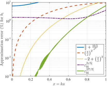
Figure 1: Approximation error ($\%$) between conditions of Eq. (8) (blue solid), second term of Eq. (15) (red dashed), the first two terms of Eq. (15) (yellow dotted), Eq. (13) (purple dot-dashed), and Eq. (15) (green-solid) with respect to the values obtained from the Mie coefficients of Eq. (2) for the first magnetic dipole. Equation. (15) gives less than $1\%$ error for values up to $x=0.8$.

Up to this point some simple rules regarding the first electric and magnetic dipole resonances have been derived. Arguably, expressions (5) and (6) are purely imaginary quantities for the lossless case, thus energy conservation is violated–see Capolino (2009) (Ch.8, p.6). This can be immediately restored by introducing higher Padé approximants, e.g. [3/3] for $a_{1}$ and [5/5] for $b_{1}$, viz.,

$$a_{1}^{[3/3]}=-i\frac{2}{3}\frac{\varepsilon_{c}-1}{\varepsilon_{c}+2}\frac{x^{3}}{\left(1-\frac{3}{5}\frac{\varepsilon_{c}-2}{\varepsilon_{c}+2}x^{2}-i\frac{2}{3}\frac{\varepsilon_{c}-1}{\varepsilon_{c}+2}x^{3}\right)}$$ (9)

$$b_{1}^{[5/5]}=-i\frac{\varepsilon_{c}-1}{45}$$ (10)

$$\frac{x^{5}}{\left(1+\frac{1}{21}(5-2\varepsilon_{c})x^{2}+[x]^{4}-i\frac{1}{45}(\varepsilon_{c}-1)x^{5}\right)}$$

where $[x]^{4}=-\frac{\varepsilon_{c}^{2}+100\varepsilon_{c}-125}{2205}x^{4}$.

Terms found in the denominator of Eq. (9) and (10) can be categorized into two types: real terms describing the dynamic depolarization effects Meier and Wokaun (1983), and imaginary terms representing the radiative damping effects de Vries et al. (1998), respectively. Notice that for $a_{1}$ and $b_{1}$ the [3/3] and [5/5] Padé approximants are the lowest order approximants with an imaginary term in their denominator; these terms appear also in the Taylor expansion–see Eq. (3), and (4). In a sense, the form and order of the radiative damping term is known once the first Taylor term is calculated.

Following the previous analysis, Eq. (9) gives the following pole condition

$$\varepsilon_{a_{1}}^{[3/3]}=-2-\frac{12}{5}x^{2}-2ix^{3}+...$$ (11)

where the imaginary term appeared reveals that a complex pole is expected, even for the lossless case due to radiative damping effects Osipov and Tretyakov (2015). This expression elucidates the fact that Mie coefficients exhibit resonances at complex frequencies, known also as natural frequencies Stratton (2007), offering an equivalent definition for these frequencies and a clear interpretation from a material point of view.

Let us continue by assuming material losses, i.e.,$\varepsilon_{c}(\omega)=\varepsilon^{\prime}(\omega)+i\varepsilon^{\prime\prime}(\omega)$. The estimated imaginary part of Eq. (11) reveals another interesting fact: the amount of dissipative losses required for maximum absorption efficiency are dictated by the amount of the radiative damping losses. This can be understood as a matching process between the two mechanisms involved, i.e., radiative damping and material dissipative losses Tribelsky (2011); Tretyakov (2014). This interchange raises a series of interesting and peculiar phenomena affecting the overall absorptive behavior of a sphere Luk’Yanchuk et al. (2012). Therefore, the required material losses for maximum absorption for the first plasmonic resonance can be approximately estimated to be

$$\varepsilon^{\prime\prime}(\omega)\approx 2x^{3}$$ (12)

Similarly, the pole of Eq. (13), rounded to the fourth decimal digit, reads

$$\varepsilon_{b_{1}}^{[5/5]}= -2.0743+\left(\frac{3.1614}{x}\right)^{2}-1.4263x^{2}+...$$ (13)

$$-i2x\left(1.0673-0.7721x^{2}+0.4604x^{4}\right)+...$$

where up to $x^{2}$ dynamic depolarization (real part) and $x^{5}$ radiative damping terms (imaginary part) are included, respectively. A first rough approximation for maximum absorption reads (see Osipov and Tretyakov (2015))

$$\varepsilon^{\prime\prime}(\omega)\approx 2x$$ (14)

easily derived by neglecting the higher order imaginary terms of Eq. (13).

Consider now the estimated radiative damping terms of Eq. (13). These, non-trivial terms predict a non-linear trend for the maximum absorption curve. Indeed, as can be seen in Fig. 2, a maximum absorption plateau is observed around $x=0.6$. We characterize this predicted plateau as a manifestation of a self-regulating radiative damping process. This is justified from the point that radiative damping is an intrinsic mechanism, affected only by the size characteristics in the small size limit, with immediate effects on the scattering and absorption processes. Hence, this non-linear trend extracted in Eq. (13) reflects the ability of a sphere to exhibit different qualitative radiative damping behavior of these two types of resonances. Note that similar effects are not observed for the electric plasmonic resonances, where the absorption maximum curve is strictly monotonous for size parameters up to $x<1$, as can be observed in Fig. 2 (green curve).

So far the proposed approximation has offered simple and compact expansions for both Mie coefficients. These features are mostly derived using the lowest Padé approximants. In order to increase the accuracy of the extracted conditions of the magnetic resonances, higher order approximants are needed. For instance a [27/2] expansion of $b_{1}$ yields to the following pole condition

$$\varepsilon_{b_{1}}^{[27/2]}= -2+\left(\frac{\pi}{x}\right)^{2}+1.696x^{2}-1.1232x^{4}+...$$ (15)

$$-i2x(1-0.696x^{2}+0.4447x^{4})+...$$

A comparison between the estimated approximations (Fig. 1) reveals that Eq. (15) gives highly accurate results, while the accuracy is still high by including only the first two terms of Eq. (15). Note that in coefficient expansions like (13) or higher, more than one poles are predicted. For a given physical system some of the predicted poles may not be observed directly, making their physical interpretation a difficult task Masjuan et al. (2014). Additionally, some of the poles may coincide with system zeros, hence their effects are canceled. Our study is restricted only for physically observable poles, verified through the analytical Mie solution.

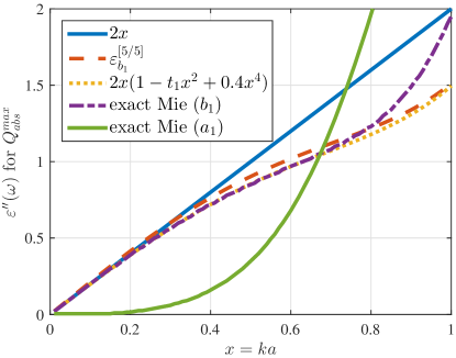
Figure 2: Calculated $\varepsilon^{\prime\prime}(\omega)$ values as a function of size parameter for maximum absorption for the first magnetic term ($b_{1}$). Blue solid line: the linear trend of Eq. (14). Red dashed line: the estimation given by Eq. (13). Yellow dotted line: the estimation given by Eq. (15); $t_{1}$ value can be found in Table I. Purple dot-dashed line illustrates the absorption trend extracted from the exact Mie coefficient (Eq. (2)). The corresponding absorption maximum for the first electric Mie term (Eq. (1) green solid) exhibiting a monotonous, $2x^{3}$ distribution. The absorption plateau is visible for $0.4<x<0.8$.

We conclude our discussion by generalizing the extracted results for the case of higher order magnetic resonances. A simple pattern regarding their resonant condition can be extracted by carefully analyzing the higher order Padé approximants and their poles, viz.,

$$\varepsilon_{bn}=-\frac{2}{2n-1}+\left(\frac{c_{n}}{x}\right)^{2}-i\frac{2}{\left[(2n-1)!!\right]^{2}}x^{2n-1}\left(1-t_{n}x^{2}\right)$$ (16)

where $n=1,2,3,...$ is the order of each mode; $c_{n}$ and $t_{n}$ values are given in the following table.

Table 1: Coefficients of Eq. (16)

$n$	1	2	3	4	5
$c_{n}$	$\pi$	4.4934	5.7634	6.9879	8.1825
$t_{n}$	0.6960	0.2507	0.1578	0.1165	0.0928

The real part of Eq. (16) is a rule for the resonant position; the absorption maximum for each mode can be approximately described by the imaginary part. Notice that $c_{n}$ coefficients follow the order of the first zero of spherical Bessel function ($j_{n-1}\left(c_{n}\right)=0$).

A new, Padé approximant-based system ansatz has been introduced for the Mie coefficients, describing the scattering and absorptive mechanisms in a homogeneous sphere. Novel aspects and accurate trends for the magnetic multipoles resonant locations were revealed, while simple and compact coefficient expansions were introduced. This perspective can be further generalized for dispersive material models Kreibig and Vollmer (1995), inhomogeneities Monticone and Alù (2014), anisotropies Wallén et al. (2015), or other geometries Ruan and Fan (2010), revealing potentially interesting and unknown radiation/light scattering phenomena. Consequently, new design guidelines will emerge regarding the scattering and absorptive functionalities of single, canonical shaped scatterers.

This work is supported by the Aalto Energy Efficiency Program (EXPECTS project) and the Aalto ELEC Doctoral School scholarship.

References

- Fan et al. (2014) X. Fan, W. Zheng, and D. J. Singh, Light Sci. Appl. 3, e179 (2014).
- Tribelsky and Luk’yanchuk (2006) M. I. Tribelsky and B. S. Luk’yanchuk, Phys. Rev. Lett. 97, 1 (2006).
- Luk’yanchuk et al. (2010) B. Luk’yanchuk, N. I. Zheludev, S. A. Maier, N. J. Halas, P. Nordlander, H. Giessen, and C. T. Chong, Nat. Mater. 9, 707 (2010).
- Jahani and Jacob (2016) S. Jahani and Z. Jacob, Nature Nanotechnology 11, 23 (2016).
- Geffrin et al. (2012) J. M. Geffrin, B. García-Cámara, R. Gómez-Medina, P. Albella, L. S. Froufe-Pérez, C. Eyraud, A. Litman, R. Vaillon, F. González, M. Nieto-Vesperinas, J. J. Sáenz, and F. Moreno, Nat. Comm. 3, 1171 (2012).
- Rayleigh (1871) J. W. S. B. Rayleigh, Phil. Mag., series 4 41, 447 (1871).
- Kerker (2013) M. Kerker, The Scattering of Light and Other Electromagnetic Radiation: Physical Chemistry: A Series of Monographs, Vol. 16 (Academic press, 2013).
- Bohren and Huffman (2008) C. F. Bohren and D. R. Huffman, Absorption and scattering of light by small particles (John Wiley & Sons, 2008).
- Stratton (2007) J. A. Stratton, Electromagnetic theory (John Wiley & Sons, 2007).
- Sihvola (2006) A. H. Sihvola, Prog. In Electromagn. Res. 62, 317 (2006).
- Meier and Wokaun (1983) M. Meier and A. Wokaun, Optic. Lett. 8, 581 (1983).
- Capolino (2009) F. Capolino, Theory and phenomena of metamaterials (CRC Press, 2009).
- García-Etxarri et al. (2011) A. García-Etxarri, R. Gómez-Medina, L. S. Froufe-Pérez, C. López, L. Chantada, F. Scheffold, J. Aizpurua, M. Nieto-Vesperinas, and J. J. Sáenz, Opt. Express 19, 4815 (2011), arXiv:1005.5446 .
- Baker and Graves-Morris (1996) G. A. Baker and P. R. Graves-Morris, Padé approximants, Vol. 59 (Cambridge University Press, 1996).
- Zunckel and Clarkson (2008) C. Zunckel and C. Clarkson, Phys. Rev. Lett. 101, 181301 (2008).
- Samuel et al. (1995) M. Samuel, J. Ellis, and M. Karliner, Phys. Rev. Lett. 74, 4380 (1995).
- Masjuan et al. (2014) P. Masjuan, J. Ruiz de Elvira, and J. J. Sanz-Cillero, Phys. Rev. D 90, 097901 (2014).
- Wiscombe (1980) W. J. Wiscombe, Appl. Optic. 19, 1505 (1980).
- Alam and Massoud (2006) M. Alam and Y. Massoud, IEEE Trans. Nanotechnol. 5, 491 (2006).
- Ambrosio and Hernández-Figueroa (2012) L. A. Ambrosio and H. E. Hernández-Figueroa, IEEE Trans. Nanotechnol. 11, 1217 (2012).
- Mei et al. (2013) Z. Mei, T. K. Sarkar, and M. Salazar-Palma, IEEE Antenn. Wireless Propag. Lett. 12, 1228 (2013).
- Tretyakov (2014) S. Tretyakov, Plasmonics , 935 (2014), arXiv:1312.0899 .
- Tribelsky (2011) M. I. Tribelsky, Europhys. Lett. 94, 14004 (2011).
- de Vries et al. (1998) P. de Vries, D. V. van Coevorden, and A. Lagendijk, Rev. Mod. Phys. 70, 447 (1998).
- Osipov and Tretyakov (2015) A. V. Osipov and S. A. Tretyakov, in 2015 1st URSI Atl. Radio Sci. Conf. (URSI AT-RASC) (IEEE, 2015).
- Luk’Yanchuk et al. (2012) B. S. Luk’Yanchuk, A. E. Miroshnichenko, M. I. Tribelsky, Y. S. Kivshar, and A. R. Khokhlov, New J. Phys. 14 (2012).
- Kreibig and Vollmer (1995) U. Kreibig and M. Vollmer, Optical properties of metal clusters (Springer-Verlag, 1995).
- Monticone and Alù (2014) F. Monticone and A. Alù, Phys. Rev. Lett. 112, 1 (2014).
- Wallén et al. (2015) H. Wallén, H. Kettunen, and A. Sihvola, Radio Sci. 50, 18 (2015).
- Ruan and Fan (2010) Z. Ruan and S. Fan, Phys. Rev. Lett. 105, 013901 (2010).