QSWalk: a Mathematica package for quantum stochastic walks on arbitrary graphs

Abstract

We present a Mathematica package, QSWalk, to simulate the time evaluation of Quantum Stochastic Walks (QSWs) on arbitrary directed and weighted graphs. QSWs are a generalization of continuous time quantum walks that incorporate both coherent and incoherent dynamics and as such, include both quantum walks and classical random walks as special cases. The incoherent component allows for quantum walks along directed graph edges. The dynamics of QSWs are expressed using the Lindblad formalism, originally developed for open quantum systems, which frames the problem in the language of density matrices. For a QSW on a graph of $N$ vertices, we have a sparse superoperator in an $N^{2}$-dimensional space, which can be solved efficiently using the built-in MatrixExp function in Mathematica. We illustrate the use of the QSWalk package through several example case studies.

PROGRAM SUMMARY

Program Title: QSWalk.m
Licensing provisions: none
Programming language: Mathematica.
Computer and operating system: any system running Mathematica Version 10 (or later).
RAM: depends on graph size.
Classification: 4.15.
Nature of problem:
The QSWalk package provides a method for simulating quantum stochastic walks on arbitrary (directed/undirected, weighted/unweighted) graphs.
Solution method:
For an $N$-vertex graph, the solution of a quantum stochastic walk can be expressed as an $N^{2}\times N^{2}$ sparse matrix exponential. The QSWalk package makes use of Mathematica’s sparse linear algebra routines to solve this efficiently.
Restrictions:
The size of graphs that can be treated is constrained by available memory.
Running time:
Running time depends on the size of the graph and the propagation time of the walk.

1 Introduction

Over the past two decades, quantum computing and information theory have emerged as one of the most exciting and promising frontiers of research, at the forefront of both quantum physics and computer science (see, e.g. [1] and references therein). One particularly interesting avenue of research is the quantum walk (QW) [2, 3, 4, 5], a quantum mechanical analogue of the classical random walk (CRW). CRWs model the random motion of a “walker” over the vertices of some graph, with each step chosen at random from the edges connecting to adjacent vertices [6, 7]. The CRW is ubiquitous throughout physics and applied mathematics, being associated with phenomena as diverse as Brownian motion in liquids [8] and price fluctuations in financial markets [9].

QWs were first described by Aharanov in 1993 et al. [10], who introduced a discrete-time formulation in which random steps are effected by means of a unitary coin operator [11, 12]. A continuous-time model, with no need of a coin operator, was subsequently introduced by Farhi and Gutmann in 1998 [13]. The key difference of both discrete- and continuous-time QWs with respect to the equivalent CRW is that the QW evolves according to quantum amplitudes instead of probabilities, and so the diffusion process of the CRW is replaced by a phase-coherent unitary evolution in which different paths can interfere. This phase-coherence leads to drastically different behaviour, which has been exploited to develop algorithms on QWs achieving an exponential speedup vis-à-vis the corresponding CRW [14].

A significant limitation of QWs is that the time evolution must be unitary in order to conserve probability. This presents a particular challenge when attempting to apply the QW to directed graphs, i.e. graphs containing edges which can only be traversed in one direction. While there have been several approaches to extend discrete-time QWs to directed graphs [15, 16], these do not carry over to the continuous-time case.

One approach that does yield a version of continuous-time QWs applicable to directed graphs is the so-called Quantum Stochastic Walk (QSW), a generalization of both QWs and CRWs developed by Whitfield et al. [17]. The object of study in a QSW is the density matrix, which combines the coherent dynamics of quantum mechanical states with the incoherent evolution of a probability vector. The QSW posits a master equation comprising a combination of the QW Hamiltonian, representing unitary evolution, and a term describing incoherent scattering. The latter is based on the Lindblad formalism from open quantum systems theory [18, 19]. By tuning the relative weighting of these components, the QSW can describe a continuum of behavior with the QW and CRW at either end. Importantly, the incoherent scattering component of the QSW is not subject to the same constraints as the Hamiltonian of the QW and is thus able to represent irreversible scattering, e.g. along one-way edges in directed graphs. QSWs have recently been applied to several problems at the forefront of current quantum information theory research, including the quantum PageRank algorithm [20], quantum neural networks [21] and, most recently, decision-making networks [22].

In this paper we present a Mathematica package, QSWalk, for the evaluation of QSWs on arbitrary directed graphs. The numerical approach used in our package is based on vectorization of the density matrix and master equation, allowing a solution in terms of a matrix exponential for which efficient sparse matrix methods can be used. By writing our package in Mathematica we are able to make use of its extensive built-in functionality for graphs and linear algebra, making our implementation straightforward and efficient. Furthermore, Mathematica offers the advantage of an intuitive notebook environment and visualization functions, and is thus an ideal tool for exploring QSWs for either research or educational purposes.

Although a python library for quantum walks has recently been made available [23], to our knowledge there is currently no software in the public domain for the computation of QSWs. A python package, QuTiP, has been written for the study of open quantum systems [24, 25], which could potentially provide similar functionality to our package. However, it is not specifically tailored to the context of quantum walks on graphs, and it requires working in Python, so may not be as accessible as our Mathematica package.

The remainder of this paper is structured as follows. In the next section we give an overview of the basic theory underlying QSWs. In Section 3 we describe the QSWalk package and some of the computational methods used therein. We then present several illustrative applications, including a study of FMO complex in photosynthesis and the quantum Page Rank algorithm, in Section 4.

2 Theory

Our goal in this section is to present the background theory relevant to QSWs in a concise and self-contained way. We also aim to establish a clear and consistent notation, which is particularly important owing to the many different (and sometimes mutually contradictory) notations in the literature (ours is most similar to that of Refs. [17] and [26]). We start by briefly defining graphs and the associated CRWs, followed by QWs, and finish with a more detailed description of QSWs. For the sake of brevity, and because they are irrelevant to QSWs, we omit the discrete-time CRW and QW models and discuss only the continuous-time case. Throughout this section, and the rest of the paper, we work in units with $\hbar=1$.

2.1 Classical random walks on graphs

For our purposes, a graph $G$ is defined as a set of vertices (or nodes) $\{1,\ldots,N\}$ together with an $N\times N$-dimensional adjacency matrix $A$ describing the connections (or edges) between them. In the simplest case of an unweighted graph, $A_{ij}=1$ if there is an edge from $j$ to $i$ and $0$ otherwise. For a $weighted$ graph, on the other hand, edges have arbitrary weights $A_{ij}>0$ representing the strength of the connection from $j$ to $i$. If $A$ is symmetric, so that $A_{ij}=A_{ji}$ for all $i,j$, $G$ is said to be undirected; otherwise it is a directed graph (or digraph). For each vertex, the sum of weights for all edges leaving it is called its out-degree: $\mathrm{outDeg}(j)=\sum_{i\neq j}A_{ij}$.

We note that the diagonal entries $A_{ii}$ represent self-loops, edges which start and finish at the same vertex; if $G$ has no self-loops it is called simple. In the literature on QWs and QSWs simple graphs are usually considered, however, non-simple graphs can in principle be used.

A (continuous-time) CRW on $G$ may be defined as an $N$-component probability vector $\mathbf{p}(t)$ whose components $p_{i}(t)$ sum to unity and represent the probability for the hypothetical walker being found at vertex $i$ at time $t$. The initial condition typically places the walker on a particular vertex at time zero, $p_{i}(0)=\delta_{i,q}$ for some $q$. The time evolution of $\mathbf{p}(t)$ is governed by a master equation:

$$\frac{\mathrm{d}\mathbf{p}}{\mathrm{d}t}=-M\cdot\mathbf{p}(t),$$ (1)

with generator matrix $M$:

$$M_{ij}=\begin{cases}-\gamma A_{ij},&i\neq j,\\ \gamma\,\mathrm{outDeg}(j),&i=j.\end{cases}$$ (2)

The parameter $\gamma>0$ determines the CRW transition rate between vertices. The off-diagonal elements of $M_{ij}$ represent the individual probability flows $j\rightarrow i$ along each edge from vertex $j$, while the diagonal elements $M_{jj}$ account for the total outflow from vertex $j$ per unit time.

The solution of Eq. (1) can be expressed as a matrix exponential:

$$\mathbf{p}(t)=\mathrm{e}^{-Mt}\cdot\mathbf{p}(0).$$ (3)

2.2 Quantum walks

A QW may be defined in a natural way by analogy to the CRW. The graph structure of $G$ is mapped onto a quantum mechanical Hilbert space in which the set of vertices forms an orthonormal basis $\{\left|1\right>,\ldots,\left|N\right>\}$. The probability vector $\mathbf{p}(t)$ from the CRW is replaced by a quantum state vector of probability amplitudes:

$$\left|\psi(t)\right>=\sum_{i=1}^{N}\left|i\right>\left<i|\psi(t)\right>.$$ (4)

The amplitudes $\left<i|\psi(t)\right>$ represent a coherent superposition over all vertices, such that the probability associated with vertex $i$ at time $t$ is $|\left<i|\psi(t)\right>|^{2}$. The CRW master equation (Eq. 1) is replaced by a Schrödinger equation:

$$\frac{\mathrm{d}\left|\psi(t)\right>}{\mathrm{d}t}=-\mathrm{i}\hat{H}\left|\psi(t)\right>,$$ (5)

where $\hat{H}$ is the Hamiltonian, whose matrix elements come from the CRW generator matrix:

$$\left<i\right|\hat{H}\left|j\right>=M_{ij}.$$ (6)

In the last two equations we have introduced the $\hat{}$ notation to denote that we regard $\hat{H}$ as an operator, independent of any basis. However, in the remainder of this paper we will switch freely between the operator ($\hat{H}$) and matrix ($H$) viewpoints depending on the context; the distinction is generally not significant.

The imaginary $\mathrm{i}$ factor on the right hand side of Eq. (5) is responsible for the uniquely “quantum” properties of the QW. It should be noted that, in order for the time evolution of the QW to be unitary (and hence probability-conserving), $\hat{H}$ must be Hermitian. From Eqs. (6) and (2), it follows that $M$ must be symmetric, and hence the graph $G$ must be undirected for a QW.

The solution to Eq. (5) can once again be expressed as a matrix exponential:

$$\left|\psi(t)\right>=\mathrm{e}^{-\mathrm{i}\hat{H}t}\left|\psi(0)\right>,$$ (7)

with the initial condition $\left|\psi(0)\right>=\left|q\right>$ for some $q$.

2.3 Quantum stochastic walks

The QW just described is restricted to undirected graphs on which the Hamiltonian operator is Hermitian. It is also, by definition, limited to pure quantum states undergoing phase-coherent unitary evolution. By contrast, the CRW represents the opposite limit, in which scattering is non-unitary and evolution is purely phase-incoherent. The QSW was proposed by Whitfield et al. [17] as a generalization that includes both QWs and CRWs as limiting special cases, and allows random walks with a combination of coherent and incoherent dynamics. The incoherent part of the QSW can be used to incorporate scattering along directed edges and thus allows directed graphs to be treated.

In place of the probability vector $\mathbf{p}(t)$ of the CRW or wavefunction $\left|\psi(t)\right>$ of the QW, the QSW is framed in terms of the density matrix $\hat{\rho}(t)$ [1, 27, 28]. In the general case, this operator describes a statistical ensemble of pure quantum states (a so-called “mixed” state):

$$\hat{\rho}(t)=\sum_{k}p_{k}\left|\psi_{k}(t)\right>\left<\psi_{k}(t)\right|.$$ (8)

The weights $p_{k}\geq 0$ satisfy $\sum_{k}p_{k}=1$ and represent the probabilities for the system to be in each of the quantum states $\left|\psi_{k}(t)\right>$. This probability reflects a lack of knowledge of the true system state, which is distinct from the quantum mechanical uncertainty associated with the measurement a single quantum state that happens to be a superposition of observable basis states. The special case of a known quantum state is recovered when only one of the $p_{k}$ is non-zero, and is known as a “pure” state.

We note several relevant properties of $\hat{\rho}(t)$ which follow from Eq. (8) and are relevant here: $\hat{\rho}(t)$ is Hermitian; $\mathrm{tr}(\hat{\rho}(t))=1$ and $\mathrm{tr}(\hat{\rho}(t)^{2})\leq 1$, with equality holding only for pure states; the expectation value of an operator $\hat{A}$ is given by $\langle\hat{A}\rangle=\mathrm{tr}(\hat{\rho}(t)\hat{A})$.

For a QSW on graph $G$, the natural representation for $\hat{\rho}(t)$ is a $N\times N$ matrix in the basis of vertex states $\{\left|1\right>,\ldots,\left|N\right>\}$, with elements $\rho_{ij}(t)=\left<i\right|\hat{\rho}(t)\left|j\right>$. As for the QW, the usual initial condition for a QSW will have the walker start in the state $\left|q\right>$ at $t=0$, so that $\hat{\rho}(0)=\left|q\right>\left<q\right|$, or equivalently, $\rho_{ij}(0)=\delta_{iq}\delta_{jq}$. For $t\geq 0$, the diagonal elements $\rho_{ii}(t)$ represent the probability density at vertex $i$ (and are therefore referred to as “populations”), while the off-diagonal elements $\rho_{ij}(t)$ ($i\neq j$) describe the phase coherence between distinct vertices $i$ and $j$ (and are known as “coherences”).

Following Ref. [17], we can now define the QSW by the following master equation:

$$\frac{\mathrm{d}\hat{\rho}}{\mathrm{d}t}=-(1-\omega)\mathrm{i}[\hat{H},\hat{\rho}(t)]+\\ \omega\sum_{k=1}^{K}\left(\hat{L}_{k}\hat{\rho}(t)\hat{L}_{k}^{\dagger}-\frac{1}{2}\left(\hat{L}_{k}^{\dagger}\hat{L}_{k}\hat{\rho}(t)+\hat{\rho}(t)\hat{L}_{k}^{\dagger}\hat{L}_{k}\right)\right),$$ (9)

where $\hat{H}$ is the Hamiltonian operator, describing coherent evolution; $\hat{L}_{k}$ are the Lindblad operators, which describe phase-incoherent scattering (see below); and $0\leq\omega\leq 1$ is a weighting factor that interpolates between the coherent and incoherent terms.

Eq. (9) is an example of the Kossakowski-Lindblad master equation [29, 30], widely used to model interactions with an external environment in the study of open quantum systems [18, 19]. In its usual context the $1-\omega$ and $\omega$ factors are not present, but it is convenient to include them in the QSW as they permit an explicit variation between completely phase coherent ($\omega=0$) and incoherent ($\omega=1$) regimes.

The first term on the right hand side of Eq. (9), representing the phase coherent component of the evolution, uses the same Hamiltonian $\hat{H}$ that we introduced in the QW. Indeed, when $\omega=0$, Eq. (9) reduces to the Liouville-von Neumann equation, which is the density matrix equivalent of the Schrödinger equation Eq. (5).

As for the QW, $\hat{H}$ must be Hermitian and hence based on an undirected graph. Unlike the QW case, however, in a QSW the graph $G$ may be undirected in general. We therefore define $\hat{H}$ in terms of a symmetrized version of $G$, as follows:

$$H_{ij}=\begin{cases}-\gamma\,\mathrm{max}(A_{ij},A_{ji}),&i\neq j,\\ -\sum_{k\neq j}H_{kj},&i=j.\end{cases}$$ (10)

The directedness of $G$ is manifest in the second term of Eq. (9), which represents the incoherent component of the evolution. It comprises a sum over the Lindblad operators $\hat{L}_{k}$, each of which corresponds to a particular scattering channel. The range of the sum, $K$, depends on the particular choice of $\{\hat{L}_{k}\}$. For a QSW, a natural choice is the set of operators representing scattering between each pair of vertices. Identifying $k$ with the pair $i,j$ (say, $k\equiv N(j-1)+i$) we define

$$\hat{L}_{k}=\sqrt{|M_{ij}|}\left|i\right>\left<j\right|,$$ (11)

representing incoherent scattering from vertex $j$ to $i$. The sum extends over all $i,j$ so that $K=N^{2}$, but only pairs with non-zero $M_{ij}$ contribute. In this way, the scattering represented by the $\hat{L}_{k}$ operators incorporates the full directed structure of $G$; this is what is meant by saying that a QSW can be applied to a directed graph. It is straightforward to show that with this set of $\hat{L}_{k}$, the QSW reduces to the CRW when $\omega=1$, if we make the obvious identification $\rho_{ii}(t)\equiv p_{i}(t)$.

Other choices for $\hat{L}_{k}$ are possible and may lead to QSWs with different physical interpretations. However, the definition in Eq. (11) is of particular interest, since it allows us to recover the well-known and widely studied QW ($\omega=0$) and CRW ($\omega=1$) as special cases. By varying $\omega$ between 0 and 1 one can then explore intermediate regimes with both quantum and classical behaviour.

3 The QSWalk package

The QSWalk package is written in the Mathematica system (also known since 2013 as the Wolfram Language) [31]. One of the key strengths of Mathematica is its vast number of built-in functions (approximately 5000 as of version 10.3), providing efficient and sophisticated numerical and symbolic algorithms.

Of particular value to our application is Mathematica’s built-in graph theory functionality: graphs are “first-class citizens” [32] and many standard graph types are available as built-in functions. This makes it easy to apply our package to immediately study a wide range of known graph types, in addition to readily defining new ones.

Mathematica also offers powerful linear algebra routines, which are essential for the efficient evaluation of QSWs. In particular, we make use of the built-in sparse array methods for the matrix exponential calculation. The use of these methods is seamless and mostly transparent to the user, which greatly streamlines the development of efficient code.

3.1 Package overview

The main purpose of the QSWalk package is the implementation of QSWs on graphs. In this section we illustrate this generic use case with a simple example that nevertheless incorporates all the necessary steps. For ease of presentation the following input and output is taken from a command-line terminal session (although we recommend working within the Mathematica notebook interface in general).

Mathematica 10.3.0 for Mac OS X x86 (64-bit)
Copyright 1988-2015 Wolfram Research, Inc.

We begin by loading the package. For this to work, the QSWalk.m file must be in the current path (as specified by the $Path variable). Alternatively, the full path to the file can be specified.

In[1]:= <<QSWalk.m

Our calculation begins by defining a graph object; here we use a built-in function to create an Erdös-Renyi random graph with 10 vertices and 30 (directed) edges:

In[2]:= G = RandomGraph[{10,30}, DirectedEdges->True];

Assuming a transition rate $\gamma=1$, we define the Hamiltonian as the generator matrix of the symmetrized graph (Eq. 10):

In[3]:= gamma = 1.;

In[4]:= H = GeneratorMatrix[UndirectedGraph[G], gamma];

We then define the Lindblad operators using the generator of the original directed graph (Eq. 11):

In[5]:= LkSet = LindbladSet[GeneratorMatrix[G,gamma]];

Next, we define the remaining inputs. The initial density matrix is $\hat{\rho}(0)=\left|1\right>\left<1\right|$, which is conveniently implemented in matrix form using the SparseArray function:

In[6]:= omega = 0.5; t = 10.;

In[7]:= rho0 = SparseArray[{{1,1}->1.}, {n,n}];

The final step is to carry out the QSW calculation:

In[8]:= rho1 = QuantumStochasticWalk[H,LkSet,omega,rho0,t];

The output is a density matrix; to get the final vertex probabilities we take the diagonal elements:

In[8]:= p = Diagonal[rho1] // Chop

Out[8]= {0.311295, 0.0266081, 0.0938145, 0.0797414, 0.0884782,

>  0.0687126, 0.0747984, 0.121446, 0.0900074, 0.0450989}

The above eight short lines of code can, with only slight modifications, be used to calculate QSWs on arbitrary graphs.

It is often of interest to evaluate a walk at a sequence of times, with the result of each time step forming the input to the next step. In this case, it is advantageous to avoid re-generating the master equation matrix for each time step. The following approach shows how this can be done in a straightforward way.

First, define a time increment dt. We then call QuantumStochasticWalk as before, but with a symbolic (i.e. undefined) initial state rho. The result is a partially evaluated expression in which the master equation has been generated, but the matrix exponential has remained unevaluated because its second argument is symbolic. We save this as a function qsw, which can subsequently be called with specific numerical values for rho:

In[12]:= dt = 1.;

In[13]:= qsw[rho_]=QuantumStochasticWalk[H,LkSet,omega,rho,dt]

Out[13]= Matricize[MatrixExp[SparseArray[<1170>, {100, 100}],
>  Vectorize[rho]]]

We use the NestList function to call qsw recursively, starting with rho = rho0 to build up a list of density matrices for each time:

In[14]:= pt = Diagonal /@ NestList[qsw,rho0,Round[t/dt]];

As a check, we can verify that the final element in this list agrees with our previous calculation:

In[20]:= Chop[Last[pt] - p]

Out[20]= {0, 0, 0, 0, 0, 0, 0, 0, 0, 0}

The Chop function is used here to zero out the small differences arising from the limitations of machine precision arithmetic.

3.2 Functions of the QSWalk package

In this section we provide a brief summary of the key functions in the QSWalk package.

Propagator functions

The function QuantumStochasticWalk implements QSWs on graphs and is the main function in the QSWalk package. We also provide functions to implement QWs and CRWs, which are much faster to evaluate (as they work with vectors of length $N$ rather than $N^{2}$) and provide a useful comparison.

• QuantumStochasticWalk[H,LkSet,omega,rho0,t]: computes a QSW with Hamiltonian matrix H, Lindblad operators LkSet, and weighting factor omega; starting from density matrix rho0 at time 0 and returning the density matrix at time t. H should be an $N\times N$ Hermitian matrix, and LkSet should be a list of $N\times N$ matrices; rho0 should be an $N\times N$ Hermitian matrix with a trace of unity.

• QuantumWalk[H,psi0,t]: computes a QW with Hamiltonian matrix H, starting from state vector psi0 at time 0 and returning the state vector at time t. H should be an $N\times N$ Hermitian matrix; psi0 should be a length-$N$ list of complex-valued probability amplitudes with squared magnitudes summing to unity.

• ClassicalRandomWalk[M,p0,t]: computes a CRW with generator matrix M, starting from probability vector p0 at time 0 and returning the probability vector at time t. M should be a real-valued $N\times N$ matrix; p0 should be a length-N list of non-negative probabilities summing to unity.

Constructing Hamiltonian and Lindblad operators

These functions are used to construct the inputs to the functions from the previous section (i.e. H, M, and LkSet).

• GeneratorMatrix[G,gamma]: returns the generator matrix $M$ for the graph G, with transition rate gamma.

• LindbladSet[mat]: returns of set of Lindblad matrices corresponding to each non-zero element of mat.

• GoogleMatrix[G,alpha]: returns the “Google matrix” with damping factor alpha for the graph G.

Vectorization functions

The following two functions convert between an $N\times N$ matrix and its $N\times 1$ vectorized form (see Section 3.3).

• Vectorize[mat]: returns the vectorization of matrix mat.

• Matricize[vec]: returns the matrix formed by applying the inverse action of the Vectorize function on vec. The length of vec must be an integer squared.

Graph functions

Here we provide definitions for several graph types that have been used in studies on quantum walks, but are not already available in Mathematica.

• CayleyTree[d,n]: returns a graph representing an $n$-th generation Cayley tree of order $d$ [33]. QWs have been applied to such graphs in the study of quantum search algorithms [34, 35].

• GluedBinaryTree[n]: returns a graph comprising two complete, $(n+1)$-level binary trees glued together in order along their leaf nodes. This graph type was used by Childs et al. as an example for which QWs provide an exponential speedup over a CRW [26].

• RandomGluedBinaryTree[n] returns a graph comprising two complete, $(n+1)$-level binary trees glued together in random order along their leaf nodes. These were important in demonstrating the existence of graphs for which no classical algorithm could compete with a quantum walk [14].

3.3 Vectorizing the master equation

We now describe our approach for solving the QSW master equation Eq. (9) in the QSWalk package. For clarity, in this section we adopt the matrix viewpoint and drop the $\hat{}$ notation throughout.

The master equation is a superoperator acting on the density matrix $\rho(t)$. In this form, a solution to Eq. (9) using the matrix exponential, by analogy to Eqs. (3, 7), cannot be found. We can, however, recast $\rho(t)$ as the $N^{2}$-element column vector $\tilde{\rho}(t)$, formed by concatenating its columns in order:

$$\tilde{\rho}(t)=(\rho_{11}(t),\ldots,\rho_{N1}(t),\rho_{12}(t),\ldots,\rho_{N2}(t),\ldots,\rho_{1N}(t),\ldots,\rho_{NN}(t))^{T}.$$ (12)

This operation is known in linear algebra as vectorization [36]. In vectorized form, Eq. (9) reduces to a linear operator (albeit in an expanded $N^{2}\times N^{2}$ space), whose solution can be expressed as a matrix exponential.

To vectorize Eq. (9) we make use of a standard identity ([36], Theorem 14.14) for arbitrary $N\times N$ matrices $X,Y,Z$:

$$\mathrm{vec}(X\cdot Y\cdot Z)=(Z^{T}\otimes X)\cdot\mathrm{vec}(Y),$$ (13)

where $\otimes$ denotes the Kronecker (direct) product, ^T is the matrix transpose, and $\cdot$ is standard matrix multiplication. The resulting vectorized QSW master equation is:

$$\frac{\mathrm{d}\tilde{\rho}}{\mathrm{d}t}=\mathcal{L}\cdot\tilde{\rho}(t)$$ (14)

where

$$\mathcal{L}=-(1-\omega)\mathrm{i}\left(I_{N}\otimes H-H^{T}\otimes I_{N}\right)+\\ \omega\sum_{k=1}^{K}\left(L_{k}^{\ast}\otimes L_{k}-\frac{1}{2}\left(I_{N}\otimes L_{k}^{\dagger}L_{k}+L_{k}^{T}L_{k}^{\ast}\otimes I_{N}\right)\right).$$ (15)

The value of this representation is that each term is a direct product involving one or more sparse matrices ($I_{N}$ and $L_{k}$), and therefore $\mathcal{L}$ is a sparse matrix. Fig. 1 illustrates this point for a complete graph, for which $H$ is dense.

Figure 1: (a) Hamiltonian matrix of a complete undirected graph with $N=8$ and random edge weights between 0 and 1; (b) the corresponding sparse matrix $\mathcal{L}$ (Eq. 15). The plots are shaded with darkness proportional to the magnitude of matrix entries, so that white areas correspond to zero entries.

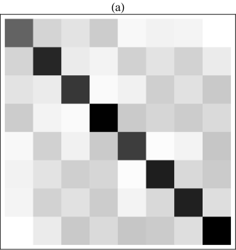
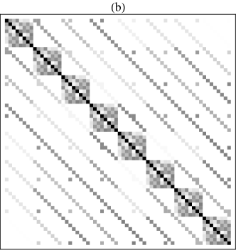
The matrix exponential solution of Eq. (14) is then

$$\tilde{\rho}(t)=\mathrm{e}^{\mathcal{L}t}\cdot\tilde{\rho}(0).$$ (16)

The density matrix $\rho(t)$ is trivially recovered from the vector $\tilde{\rho}(t)$.

Eq. (14) can be implemented using Mathematica’s built-in functions; in particular, KroneckerProduct, IdentityMatrix, Conjugate, Transpose, ConjugateTranspose, as well as matrix multiplication (the “.” operator).

The vectorization approach outlined above leads us to work with matrices of size $N^{2}\times N^{2}$, which quickly become rather large for even moderately-sized graphs. It therefore becomes essential to exploit sparse matrix representations. In Mathematica, sparse arrays are implemented via the SparseArray function [37], and all of the built-in matrix functionality includes handling to work with SparseArray objects efficiently. Therefore, provided we correctly initialize all the relevant matrices to be in SparseArray form, Mathematica will automatically carry out all matrix operations using sparse matrix methods if possible.

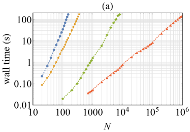
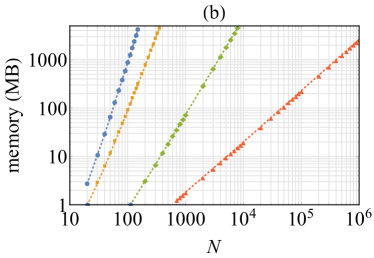
The performance of our approach depends on both the size (number of vertices) and density (number of edges) of the graph being studied. Fig. 2 gives some indicative estimates of running time and memory requirements for representative dense and sparse graphs. It can be seen that the primary bottleneck on a typical machine is memory: typically, memory requirements for a QSW can be as high as 4GB with run times of only several minutes. This corresponds to $N\approx 150$ for dense graphs, and $N\approx 350$ for sparse graphs. For QWs, unsurprisingly, the scaling is much better: for comparable run time and memory we can calculate QWs on graphs with $N\approx 10^{4}$ (dense) and $N\approx 10^{6}$ (sparse).

Figure 2: Scaling behaviour for QSWs and QWs as a function of graph size $N$, for representative examples of dense (D) and sparse (S) undirected graphs. The dense graphs have $N(N-1)/2$ edges (defined with CompleteGraph), while the sparse graphs are of Erdös-Renyi type with $\sim N\mathrm{log}N$ edges (defined with RandomGraph); in both cases the edges are assigned random weights uniformly between 0 and 1. In these figures, the slope of the lines gives the scaling exponent with respect to $N$. In (a), these are approximately (in the same order as the legend): 3.3, 2.7, 2.2, and 1.1; in (b), they are 3.7, 3.0, 2.0, and 1.1. The parameters used are $\gamma=1$, $\omega=0.5$, $t=10$, with initial conditions $\rho_{ij}(0)=\delta_{ij}/n$ (QSW) and $\left<i|\psi(0)\right>=1/\sqrt{n}$ (QW). Calculations were performed on a Late-2013 iMac with 8GB RAM, running Mathematica 10.3 on Mac OS 10.11.

4 Applications

In this section we describe several applications of the QSWalk package to systems similar to those studied recently in the literature. Our emphasis is on demonstrating the functionality of the package rather than describing any new physics.

4.1 Quantum-classical transition on a line

One of the key properties of the QSW is that it permits an interpolation between coherent (QW) and incoherent (CRW) dynamics, via the parameter $\omega$. To illustrate this transition, we consider a QSW on one of the simplest graphs possible: an undirected $N\times 1$ line graph (which is equivalent to the one-dimensional tight-binding model studied in electron transport theory [38]). The adjacency matrix for such a graph has entries $A_{ij}=\delta_{i,j+1}+\delta_{i,j-1}$. The matrix elements of the Hamiltonian and Lindblad operators can be found using Eqs. (10) and (11):

$$\left<i\right|\hat{H}\left|j\right>=\gamma\left(\delta_{ij}\left(2-\delta_{i,1}-\delta_{iN}\right)-\delta_{i,j+1}-\delta_{i,j-1}\right),$$ (17)

$$\left<i\right|\hat{L}_{k^{\prime}}\left|j\right>=\delta_{i^{\prime}i}\delta_{j^{\prime}j}\sqrt{\gamma}\left(\delta_{i^{\prime}j^{\prime}}\left(2-\delta_{i^{\prime},1}-\delta_{i^{\prime}N}\right)+\delta_{i^{\prime},j^{\prime}+1}+\delta_{i^{\prime},j^{\prime}-1}\right),$$ (18)

where $k^{\prime}\equiv(i^{\prime},j^{\prime})$ and $\hat{L}_{k^{\prime}}$ is the Lindblad operator corresponding to the scattering process $\left|i^{\prime}\right>\left<j^{\prime}\right|$. As initial condition we assume the state is localized in the middle of the line at vertex $q=(N+1)/2$ (assuming odd $N$), so that $\hat{\rho}(0)=\left|q\right>\left<q\right|$.

The code to implement this QSW in QSWalk is straightforward, and uses the built-in GridGraph function for the line graph:

n = 51; gamma = 1.; t = 10.; omega = 0.5;
G = GridGraph[{n}];
H = GeneratorMatrix[G, gamma];
LkSet = LindbladSet[H];
rho0 = SparseArray[{{(n+1)/2,(n+1)/2}->1.},{n,n}];
rho1 = QuantumStochasticWalk[H,LkSet,omega,rho0,t];

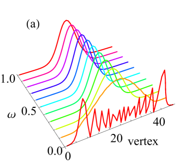
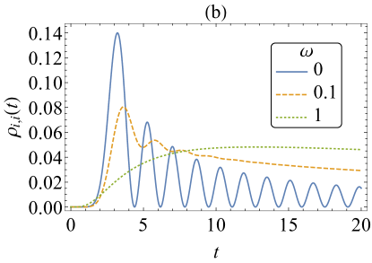
Fig. 3 shows the dynamics of the resulting QSW. In Fig. 3a, the transition from an oscillatory distribution (characteristic of coherent dynamics) at $\omega=0$, to a purely diffusive distribution at $\omega=1$, is clearly evident. Fig. 3b shows the time evolution of a particular vertex population ($i\approx 0.6N$) for several values of $\omega$, illustrating the damping which occurs when $\omega>0$. This is actually a useful property, as it causes the QSW populations to converge to a stationary state rather than oscillate indefinitely, while still retaining some (transitory) coherence.

Figure 3: (a) A sequence of QSWs showing the transition from pure QW ($\omega=0$) to pure CRW ($\omega=1$), on a line graph with $N=51$ vertices and propagation time $t=5$ (in atomic units). (b) Time evolution of QSWs on the same graph, for a fixed vertex $i=31$ ($\approx 0.6N$) for several values of $\omega$.

4.2 Pure dephasing scattering

As noted in Ref. [17], an alternative approach to incoherent scattering is via pure dephasing scattering processes [3]. In this model, the Lindblad operators are defined by

$$\hat{L}_{k}=\left|k\right>\left<k\right|,$$ (19)

for $k=1,\ldots,N$.

The implementation is the same as the previous section, with the exception of the definition of $\hat{L}_{k}$, which now reads:

LkSet = Table[SparseArray[{{i,i}->1}, {n,n}], {i,n}];

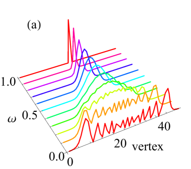
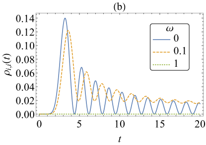
In Fig. 4 we consider a QSW using the pure dephasing model of Eq. (19) on the line graph from the previous section. There are several notable differences: firstly, from Fig. 4a it is clear that $\omega\rightarrow 1$ no longer produces the CRW. In fact, in this limit there are no dynamics at all since the $\hat{L}_{k}$ operators do not scatter between vertices. In this case, for $\omega=1$ we have $\hat{\rho}(t)=\hat{\rho}(0)$ for all $t$.

Secondly, comparing Fig. 4 to Fig. 3 we see that pure dephasing scattering causes less dephasing than the model of Eq. (11), in the sense that the wave-like oscillations persist for larger $\omega$. This is actually not surprising since for the line graph the model of Eq. (11) has dephasing terms with weighting $\sqrt{2}$ (in contrast to the weighting of $1$ in Eq. 19), in addition to the off-diagonal scattering elements which also contribute to the dephasing.

Figure 4: The equivalent of the plots from Fig. 3 but for a QSW with pure dephasing scattering (Eq. 19).

4.3 Photosynthetic light-harvesting in the FMO complex

QSWs have found application to an important problem in biophysics, concerning the capture of energy (in the form of photons from sunlight) by photosynthetic protein complexes [39]. A prototypical example which has been extensively studied is the so-called Fenna-Matthews-Olson (FMO) complex from green sulphur bacteria. This molecule is comprised of seven regions called chromophores, through which electronic excitations (excitons) are propagated by a hopping process in which phase coherence plays an important role [40]. An excitation generated by photon absorption on a particular chromophore is transmitted through the complex to a reaction centre where it is converted to stored chemical energy.

Theoretical studies aimed at understanding the phase coherence properties in the FMO have modeled the chromophores as vertices in an undirected graph on which excitons follow a quantum walk-like process [41, 42, 43] which, like the QSW, combines coherent and incoherent evolution through a master equation. These models are not strictly equivalent to QSWs as they incorporate a loss term, representing absorption of the exciton into the reaction centre, and therefore are not probability-conserving. Nevertheless, it is straightforward to develop a QSW model which describes the same essential physics, as we now show.

As a concrete example, we consider the model of Hoyer et al. [42], which uses a Hamiltonian obtained by Adolphs and Renger [44]:

$$H=\left(\begin{array}[]{ccccccc}\mathbf{200}&\mathbf{-96}&5&-4.4&4.7&-12.6&-6.2\\ \mathbf{-96}&\mathbf{320}&\mathbf{33.1}&6.8&4.5&7.4&-0.3\\ 5&\mathbf{33.1}&\mathbf{0}&\mathbf{-51.1}&0.8&-8.4&7.6\\ -4.4&6.8&\mathbf{-51.1}&\mathbf{110}&\mathbf{-76.6}&-14.2&\mathbf{-67}\\ 4.7&4.5&0.8&\mathbf{-76.6}&\mathbf{270}&\mathbf{78.3}&-0.1\\ -12.6&7.4&-8.4&-14.2&\mathbf{78.3}&\mathbf{420}&\mathbf{38.3}\\ -6.2&-0.3&7.6&\mathbf{-67}&-0.1&\mathbf{38.3}&\mathbf{230}\end{array}\right).$$ (20)

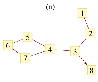
The bold entries represent the chromophores with the largest hopping probabilities, and correspond to vertices 1 to 7 of the graph shown in Fig. 5a. The units of energy are $\mathrm{cm}^{-1}$ (using the spectroscopy convention of expressing energy in terms of the wavelength of a photon with that energy, i.e. $1\mathrm{cm}^{-1}\equiv 1.23984\times 10^{-4}\mathrm{eV}$). It is also customary to work in units with $\hbar=1$, so that the unit of time is $5.309\mathrm{ps}$.

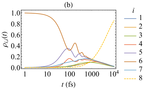
In the FMO model, the exciton is created at chromophore 6, so for our QSW we use initial condition $\hat{\rho}(0)=\left|6\right>\left<6\right|$. Chromophore 3 is the site where the exciton is absorbed into the reaction centre, which has been modeled in previous studies by including non-probability conserving “loss” terms in the master equation. Here, we take a simpler approach and add an extra vertex (labeled 8 in Fig. 5a). This “sink” vertex is connected via a directed edge to vertex 3, but it is not included in the Hamiltonian; it therefore contributes incoherent scattering via a Lindblad operator but does not participate in the coherent evolution.

Our QSW model then takes $H$ from Eq. (20) (padded with zeros to make an $8\times 8$ matrix) to describe the coherent evolution. For the incoherent evolution we use the usual set of Lindblad operators from Eq. (11) (using $H_{ij}$ in place of $M_{ij}$), representing dephasing scattering as well as incoherent scattering between chromophores; this is a slight departure from Hoyer et al. , who only included the dephasing scattering. The exciton absorption at the sink vertex is represented by an extra Lindblad operator, $\hat{L}_{k}=\sqrt{\alpha\gamma}\left|8\right>\left<3\right|$, where the factor $\alpha$ determines the rate of absorption.

In Fig. 5b we show the vertex populations as a function of time for a particular set of parameters, which demonstrates excellent qualitative agreement with Fig. 3d of Ref. [42] (whose calculation used dephasing scattering rates based on a temperature of 77K). A key feature is the damping of oscillations due to the combination of coherent and incoherent dynamics. Also evident is the accumulation of probability at the sink vertex ($i=8$), at the expense of the remaining vertices, representing the absorption of the exciton into the reaction centre. Although temperature does not appear explicitly in our model, its effect is approximated by the factor $\omega$: $\omega\rightarrow 0$ is equivalent to the low-temperature limit of a phase coherent QW, while $\omega\rightarrow 1$ corresponds to the high-temperature limit of a CRW with no phase coherence.

Figure 5: (a) Simplified graph structure of the FMO complex. (b) Vertex populations as a function of time for a QSW on the FMO model (with parameter values $\gamma=1$, $\omega=0.1$, $\alpha=100$).

4.4 Quantum Page Rank

As an interesting application of QSWs to directed graphs, we now briefly discuss the recent continuous-time quantum page rank algorithm (QPR) introduced by Sánchez-Burillo et al. [20, 45], based on the well-known (classical) Page Rank algorithm (CPR) [46] which is a key component of the Google search engine. The basic idea of CPR is to represent the world wide web as a directed graph, with each webpage representing a vertex and the links on each page representing outward edges to the pages linked to; the algorithm then carries out a CRW on this graph to determine the centrality, or “rank”, of each page. In the QPR algorithm, the CRW is replaced by a QSW which respects the directed nature of the graph.

A detailed discussion of the QPR and CPR algorithms can be found in Refs. [20, 45]; here we just describe the main features. We begin with a directed graph $G$ having $N$ vertices and adjacency matrix $A$. The Hamiltonian is defined as usual in terms of a symmetrized form of $G$ (Eq. 10). The Lindblad operators are defined in terms of the so-called “Google matrix”, $\mathcal{G}$:

$$\hat{L}_{k}=\sqrt{\gamma\mathcal{G}_{ij}}\left|i\right>\left<j\right|,$$ (21)

where

$$\mathcal{G}_{ij}=\begin{cases}\alpha A_{ij}/\mathrm{outDeg}(j)+(1-\alpha)\frac{1}{N},&\mathrm{outDeg}(j)>0,\\ \frac{1}{N},&\mathrm{outDeg}(j)=0.\end{cases}$$ (22)

The effect of $\mathcal{G}$ is to avoid “dead ends” (nodes with out-degree 0 are scattered equally to all other vertices) and to introduce random jumps between all vertices. The “damping factor” $\alpha$ controls the weighting of the random jumps relative to the edges in the original graph ($\alpha=0.85$ is a common choice in the literature).

As with all QSWs, the parameter $\omega$ determines the relative weighting of coherent and incoherent components. For $\omega=0$ we get a QW on a symmetrized graph; this does not in general provide a useful ranking algorithm, as it does not incorporate the graph directionality. For $\omega=1$, on the other hand, we recover the original CPR algorithm. For intermedate $\omega$, the QPR algorithm proceeds by evaluating the QSW (Eq. 16) from arbitrary initial conditions with $t$ large enough for $\hat{\rho}(t)$ to reach a stationary state. The vertex populations, $\rho_{ii}(t)$, then represent their rank.

The implementation using QSWalk is once again straightforward. The only new step is the definition of $\hat{L}_{k}$ (Eq. 21), for which we now use the GoogleMatrix function:

  LkSet = LindbladSet[Sqrt[gamma] GoogleMatrix[G, alpha]];

The remainder of the calculation proceeds as in Section 4.1. It is worth noting the built-in Mathematica function PageRankCentrality, which computes the CPR and is a useful reference point.

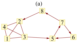
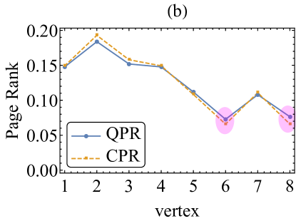
As a simple illustration, in Fig. 6 we show an example from Ref. [20]. The QPR and CPR values are broadly similar, although the QPR calculation “lifts” the degeneracy of two vertices whose ranking under CPR is equal. In Ref. [20], the authors show that this effect also holds for larger real-world networks, suggesting that QPR could become an important application for QSWs.

Figure 6: (a) The graph used by Sánchez-Burillo et al. [20] to illustrate degeneracy-breaking by the quantum page rank algorithm. (b) Quantum and classical Page Ranks of the vertices of this graph; the highlighted vertices have equal CPR but different QPR. (The parameters used in these calculations are $t=100$, $\gamma=1$, $\alpha=0.85$, $\omega=0.8$.)

5 Conclusion

The intensive research in quantum computing and information theory over recent decades has spurred interest in a range of quantum walk models such as the recently-developed quantum stochastic walks. As well as the exciting potential for practical applications down the line, these models are uncovering a wealth of interesting physics. In practice, for all but the simplest examples much of the insight is gained with the help of efficient numerical computing tools. There is thus a clear need for software packages which abstract away the computational details and allow the focus to remain on the physical application at hand. It is with this perspective in mind that we have developed the QSWalk package; we hope that it will be a useful tool, both in the hands of researchers active in this field as well as instructors wishing to bring cutting-edge models into a computer lab teaching environment.

On a typical modern desktop computer, the implementation provided by QSWalk can be applied to graphs with a few hundred vertices with calculation times on order of the tens of seconds, which should make it suitable for a wide range of applications. However, there will be specialized applications involving larger graphs where it becomes necessary to turn to high performance computing (HPC) resources (supercomputers), which would be beyond the scope of our package in its current form. One possibility for a future version of QSWalk, therefore, would be to incorporate calls to a program using parallelized linear algebra libraries running in an HPC environment; an approach along these lines was used successfully in Ref. [23] to simulate phase-coherent quantum walks.

References

- [1] M. Nielsen, I. Chuang, Quantum Computation and Quantum Information: 10th Anniversary Edition, Cambridge University Press, 2010.
- [2] J. Kempe, Quantum random walks: An introductory overview, Contemporary Physics 44 (4) (2003) 307–327.
- [3] V. Kendon, Decoherence in quantum walks – a review, Mathematical Structures in Computer Science 17 (2007) 1169–1220.
- [4] S. E. Venegas-Andraca, Quantum walks: a comprehensive review, Quantum Information Processing 11 (5) (2012) 1015–1106.
- [5] K. Manouchehri, J. Wang, Physical Implementation of Quantum Walks, Quantum Science and Technology, Springer Berlin Heidelberg, 2014.
- [6] J. Rudnick, G. Gaspari, Elements of the Random Walk: An introduction for Advanced Students and Researchers, Cambridge University Press, 2004.
- [7] P. Blanchard, D. Volchenkov, Random Walks and Diffusions on Graphs and Databases: An Introduction, Springer Series in Synergetics, Springer Berlin Heidelberg, 2011.
- [8] A. Einstein, Investigations on the Theory of the Brownian Movement, Dover Books on Physics Series, Dover Publications, 1956.
- [9] B. G. Malkiel, A Random Walk Down Wall Street, Norton, 1999.
- [10] Y. Aharonov, L. Davidovich, N. Zagury, Quantum random walks, Phys. Rev. A 48 (1993) 1687–1690.
- [11] D. Aharonov, A. Ambainis, J. Kempe, U. Vazirani, Quantum walks on graphs, in: Proceedings of the Thirty-third Annual ACM Symposium on Theory of Computing, STOC ’01, ACM, New York, NY, USA, 2001, pp. 50–59.
- [12] A. Ambainis, E. Bach, A. Nayak, A. Vishwanath, J. Watrous, One-dimensional quantum walks, in: Proceedings of the Thirty-third Annual ACM Symposium on Theory of Computing, STOC ’01, ACM, New York, NY, USA, 2001, pp. 37–49.
- [13] E. Farhi, S. Gutmann, Quantum computation and decision trees, Phys. Rev. A 58 (1998) 915–928.
- [14] A. M. Childs, R. Cleve, E. Deotto, E. Farhi, S. Gutmann, D. A. Spielman, Exponential algorithmic speedup by a quantum walk, in: Proceedings of the Thirty-fifth Annual ACM Symposium on Theory of Computing, STOC ’03, ACM, New York, NY, USA, 2003, pp. 59–68.
- [15] M. Szegedy, Spectra of quantized walks and a -rule, arXiv preprint quant-ph/0401053.
- [16] A. Montanaro, Quantum walks on directed graphs, Quantum Inf. Comp 7 (2007) 93–102.
- [17] J. D. Whitfield, C. A. Rodríguez-Rosario, A. Aspuru-Guzik, Quantum stochastic walks: A generalization of classical random walks and quantum walks, Phys. Rev. A 81 (2010) 022323.
- [18] H. Breuer, F. Petruccione, The Theory of Open Quantum Systems, Oxford University Press, 2002.
- [19] Á. Rivas, S. Huelga, Open Quantum Systems: An Introduction, SpringerBriefs in Physics, Springer Berlin Heidelberg, 2011.
- [20] E. Sánchez-Burillo, J. Duch, J. Gómez-Gardeñes, D. Zueco, Quantum navigation and ranking in complex networks, Scientific Reports 2 (2012) 605.
- [21] M. Schuld, I. Sinayskiy, F. Petruccione, Quantum walks on graphs representing the firing patterns of a quantum neural network, Phys. Rev. A 89 (2014) 032333.
- [22] I. Martínez-Martínez, E. Sánchez-Burillo, Quantum stochastic walks on networks for decision-making, Scientific Reports 6 (2016) 23812.
- [23] J. A. Izaac, J. B. Wang, pyctqw: A continuous-time quantum walk simulator on distributed memory computers, Computer Physics Communications 186 (0) (2015) 81–92.
- [24] J. Johansson, P. Nation, F. Nori, Qutip: An open-source python framework for the dynamics of open quantum systems, Computer Physics Communications 183 (8) (2012) 1760 – 1772.
- [25] J. Johansson, P. Nation, F. Nori, Qutip 2: A python framework for the dynamics of open quantum systems, Computer Physics Communications 184 (4) (2013) 1234 – 1240.
- [26] A. M. Childs, E. Farhi, S. Gutmann, An example of the difference between quantum and classical random walks, Quantum Information Processing 1 (1-2) (2002) 35–43.
- [27] M. Bellac, P. de Forcrand-Millard, Quantum Physics, Cambridge University Press, 2011.
- [28] J. Sakurai, J. Napolitano, Modern Quantum Mechanics, Pearson new international edition, Pearson, 2013.
- [29] A. Kossakowski, On quantum statistical mechanics of non-hamiltonian systems, Reports on Mathematical Physics 3 (4) (1972) 247 – 274.
- [30] G. Lindblad, On the generators of quantum dynamical semigroups, Comm. Math. Phys. 48 (2) (1976) 119–130.
- [31] S. Wolfram, An Elementary Introduction to the Wolfram Language, Wolfram Media, Incorporated, 2016.
- [32] Graphs & Networks -— Wolfram Language Documentation, https://reference.wolfram.com/language/guide/GraphsAndNetworks.html.
- [33] M. Ostilli, Cayley trees and bethe lattices: A concise analysis for mathematicians and physicists, Physica A: Statistical Mechanics and its Applications 391 (12) (2012) 3417 – 3423.
- [34] E. Agliari, A. Blumen, O. Muelken, Quantum-walk approach to searching on fractal structures, Physical Review A 82 (1) (2010) 012305.
- [35] S. D. Berry, J. B. Wang, Quantum-walk-based search and centrality, Phys. Rev. A 82 (2010) 042333.
- [36] S. Banerjee, A. Roy, Linear Algebra and Matrix Analysis for Statistics, Chapman & Hall/CRC Texts in Statistical Science, CRC Press, 2014.
- [37] SparseArray —- Wolfram Language Documentation, https://reference.wolfram.com/language/ref/SparseArray.html.
- [38] S. Datta, Electronic Transport in Mesoscopic Systems, Cambridge Studies in Semiconductor Physics, Cambridge University Press, 1997.
- [39] R. Blankenship, Molecular Mechanisms of Photosynthesis, Wiley, 2014.
- [40] G. S. Engel, T. R. Calhoun, E. L. Read, T.-K. Ahn, T. Mančal, Y.-C. Cheng, R. E. Blankenship, G. R. Fleming, Evidence for wavelike energy transfer through quantum coherence in photosynthetic systems, Nature 446 (7137) (2007) 782–786.
- [41] M. Mohseni, P. Rebentrost, S. Lloyd, A. Aspuru-Guzik, Environment-assisted quantum walks in photosynthetic energy transfer, The Journal of chemical physics 129 (17) (2008) 174106.
- [42] S. Hoyer, M. Sarovar, K. B. Whaley, Limits of quantum speedup in photosynthetic light harvesting, New Journal of Physics 12 (6) (2010) 065041.
- [43] M. B. Plenio, S. F. Huelga, Dephasing-assisted transport: quantum networks and biomolecules, New Journal of Physics 10 (11) (2008) 113019.
- [44] J. Adolphs, T. Renger, How proteins trigger excitation energy transfer in the fmo complex of green sulfur bacteria, Biophysical journal 91 (8) (2006) 2778–2797.
- [45] T. Loke, J. Tang, J. Rodriguez, M. Small, J. Wang, Comparing classical and quantum pageranks, arXiv preprint arXiv:1511.04823.
- [46] S. Brin, L. Page, Reprint of: The anatomy of a large-scale hypertextual web search engine, Computer networks 56 (18) (2012) 3825–3833.