Scale-free networks with exponent one

Abstract

A majority of studied models for scale-free networks have degree distributions with exponents greater than $2$. Real networks, however, can demonstrate essentially more heavy-tailed degree distributions. We explore two models of scale-free equilibrium networks that have the degree distribution exponent $\gamma=1$, $P(q)\sim q^{-\gamma}$. Such degree distributions can be identified in empirical data only if the mean degree of a network is sufficiently high. Our models exploit a rewiring mechanism. They are local in the sense that no knowledge of the network structure, apart from the immediate neighbourhood of the vertices, is required. These models generate uncorrelated networks in the infinite size limit, where they are solved explicitly. We investigate finite size effects by the use of simulations. We find that both models exhibit disassortative degree–degree correlations for finite network sizes. In addition, we observe a markedly degree-dependent clustering in the finite networks. We indicate a real-world network with a similar degree distribution.

I Introduction

Scale-free networks have been in the forefront of networks research for almost two decades. Examples range from social networks Newman (2001); Liljeros et al. (2001), biological networks Albert (2005); Eguiluz et al. (2005) to artificial networks like the internet Faloutsos et al. (1999) and the world-wide web Albert et al. (1999); Barabási et al. (2000). The widely accepted mechanism for the evolution of growing scale-free networks is preferential attachment Barabási and Albert (1999). This mechanism has been extensively explored and many generalizations and modifications of the original model have been suggested Dorogovtsev et al. (2000); Krapivsky et al. (2000); Albert and Barabási (2002); Dorogovtsev and Mendes (2002, 2003). The same principle has also been applied to equilibrium networks Dorogovtsev et al. (2003). The preferential attachment mechanism has relations with random multiplicative processes (Adamic and Huberman (2000); Levy and Solomon (1996); Sornette (1998); Mitzenmacher (2004)) which have relevance in many fields of statistical physics, and are known to produce skewed distributions. Besides preferential attachment, some other methods of producing scale-free networks have been exploited, for example, fitness-based models Bianconi and Barabási (2001a, b); Caldarelli et al. (2002), merging processes Kim et al. (2005); Alava and Dorogovtsev (2005); Seyed-Allaei et al. (2006), optimization models Valverde et al. (2002); D’Souza et al. (2007), urn-based statistical ensembles Burda et al. (2001); Burda and Krzywicki (2003), networks embedded into metric spaces Krioukov et al. (2010); Papadopoulos et al. (2012), and others.

Most well-studied real networks appear to have degree distribution exponents larger than two. As a result, and also due to the popularity of the preferential attachment mechanism, networks with smaller exponents have received much less attention. In such networks the mean degree diverges, and consequently the “natural” cutoff of the degree distribution scales with the system size in a different way compared to networks with higher exponents Seyed-Allaei et al. (2006). The case of $\gamma=1$ is even more peculiar: the normalization condition implies that the cutoff of the degree distribution must remain finite in an infinite system. This circumstance makes it rather difficult to clearly identify such distributions in empirical data obtained from sparse networks. On the other hand, if the mean vertex degree is sufficiently large, this kind of distribution can be observed (see below), which justifies our investigation. To our knowledge, the only studied model for networks with $\gamma=1$, was that of trees growing based on “the power of choice” (local optimization of the new connections) D’Souza et al. (2007). Note that variations of the models with hidden variables Zuev et al. (2016); Colomer-de Simon and Boguná (2012); Anand et al. (2014) can also generate such degree distributions if one chooses an appropriate distribution of hidden variables.

In the present paper we consider two simple equilibrium network models producing $\gamma=1$. These rewiring models are local in the sense that the vertices need to “know” only the structure of their immediate neighbourhoods. We show that the resulting degree distribution has a simple exact solution in the sparse network limit, where the network is uncorrelated, which is a power-law of $\gamma=1$ with an exponential cutoff that is determined by the mean degree. We perform extensive numerical simulations of these models for finite networks, and observe marked disassortative degree–degree correlations.

Figure 1: Schematic representation of the evolution mechanism for models $1$ and $2$.

II The models

A well-studied class of mechanisms that is known to produce power-law distributions, is random multiplicative processes Adamic and Huberman (2000); Levy and Solomon (1996); Sornette (1998); Mitzenmacher (2004). The essence of such models is that the fluctuations of random variables are proportional to their values (independent fluctuations would result in classical Brownian dynamics). A simple example of such processes is discussed in Pietronero et al. (2001) and is shown to generate power-law distributions of exponent 1. We use a similar principle. In our case, the random variables are the degrees of nodes in the network. Instead of fluctuations which are proportional to the values of the random variables, we apply fluctuations of a fixed size (rewiring one link at a time) with a probability that is proportional to the values of the random variables (degrees of nodes). Here we consider a model of equilibrium networks that realizes this scheme.

Model 1. Consider an arbitrary connected graph. At every step of the evolution do the following:

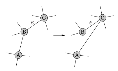
1. Choose an edge uniformly at random (edge $e$ in Fig. 1).

2. Reattach a neighbour (node $A$ in Fig. 1) of one of its end nodes to the other (from node $B$ to node $C$ in Fig. 1).

Repeat the above procedure until equilibrium is reached. In the second step node $A$ is chosen uniformly at random from the set of all neighbours of $B$ which are not neighbours of $C$ (and are not themselves $C$). If there are no such nodes, then nothing should be done in this iteration.

We denote the degree distribution by $P(q)$. The joint degree distribution, i.e., the probability that the end nodes of a uniformly randomly chosen link have degrees $q$ and $q^{\prime}$ is denoted by $P(q,q^{\prime})$, and the conditional probability that an end node of a random link has degree $q$ given that the other end node has degree $q^{\prime}$, by $P(q|q^{\prime})$. In a given step of the evolution the probability of a node of degree $q$ to be chosen as node $B$ is

$$P_{B}(q)=\frac{1}{2}\frac{qP(q)}{\langle q\rangle}$$ (1)

and, similarly, the probability of a node of degree $q$ to be chosen as node $C$ is

$$P_{C}(q)=\frac{1}{2}\frac{qP(q)}{\langle q\rangle}=P_{B}(q).$$ (2)

Assuming that in equilibrium, clustering is purely a result of degree–degree correlations, we introduce $R(q,q^{\prime})$, the probability that if a node of degree $q$ is chosen as $B$ and a node of degree $q^{\prime}$ as $C$, then a rewiring is possible, i.e., that $B$ has at least one neighbour that is not a neighbour of $C$:

$$R(1,q^{\prime}) = 0,$$

$$R(q>1,q^{\prime}) = 1-\left\lgroup\sum_{k}P(k|q)P(q^{\prime}|k)\frac{(q^{\prime}-1)(k-1)}{Nq^{\prime}P(q^{\prime})}\right\rgroup^{q-1}$$ (3)

$$= 1-\left\lgroup\frac{\langle q\rangle^{2}(q^{\prime}-1)}{Nqq^{\prime}P(q)P(q^{\prime})}\sum_{k}\frac{P(k,q)P(q^{\prime},k)(k-1)}{kP(k)}\right\rgroup^{q-1},$$

where $N$ is the number of nodes in this network. Now we can write the probability that a node of degree $q$ is chosen as $B$ and rewiring is possible:

$$P_{B,r}(1) = 0,$$

$$P_{B,r}(q>1) = \frac{1}{2}\frac{qP(q)}{\langle q\rangle}\sum_{q^{\prime}}P(q^{\prime}|q)R(q,q^{\prime}).$$ (4)

Similarly, the probability that a node of degree $q$ is chosen as $C$ and rewiring is possible:

$$P_{C,r}(q)=\frac{1}{2}\frac{qP(q)}{\langle q\rangle}\sum_{q^{\prime}>1}P(q^{\prime}|q)R(q^{\prime},q).$$ (5)

It is easy to see from Eq. (3) that in the limit $N\rightarrow\infty$, $R(q,q^{\prime})=1$ for any $q>1,q^{\prime}$ and $R(1,q^{\prime})=0$. In this case, Eq. (4) reduces to

$$P_{B,r}(1) = 0,$$

$$P_{B,r}(q>1) = \frac{1}{2}\frac{qP(q)}{\langle q\rangle},$$ (6)

and Eq. (5) becomes

$$P_{C,r}(q)=\frac{1}{2}\frac{qP(q)}{\langle q\rangle}b(q),$$ (7)

where $b(q)=1-P(1|q)$. Noting that in the stationary state the probability of a node of degree $q+1$ losing an edge must match the probability of a node of degree $q$ gaining an edge, we can write the stationary equation for the degree distribution:

$$P_{C,r}(q)=P_{B,r}(q+1).$$ (8)

Substituting Eqs. (6) and (7) into Eq. (8), we have:

$$\frac{1}{2}\frac{qP(q)}{\langle q\rangle}b(q)=\frac{1}{2}\frac{(q+1)P(q+1)}{\langle q\rangle}.$$ (9)

We see that degree–degree correlations appear only in $b(q)$. If we assume that $b(q)$ is constant (this is a weaker assumption than assuming that correlations are entirely absent), then $b(q)=c=1-1P(1)/\langle q\rangle$. This can be easily seen in the following way. For any network, regardless of degree-degree correlations, the degree distribution of end nodes of links is $qP(q)/\langle q\rangle$ (the probability, that a randomly chosen end node of a randomly chosen link has degree $q$). The probability that an end node of a randomly chosen link has degree 1, is therefore $1P(1)/\langle q\rangle$. This probability can also be written as:

$$\frac{1P(1)}{\langle q\rangle}=\sum_{q}P(1|q)\frac{qP(q)}{\langle q\rangle}.$$ (10)

Assuming that $P(1|q)$ is constant ($P(1|q)=h$), we have

$$\frac{1P(1)}{\langle q\rangle}=\sum_{q}P(1|q)\frac{qP(q)}{\langle q\rangle}=\sum_{q}h\frac{qP(q)}{\langle q\rangle}=h.$$ (11)

Therefore $b(q)=1-P(1|q)=1-1P(1)/\langle q\rangle=c$. Then Eq. (9) is simply

$$qP(q)c=(q+1)P(q+1).$$ (12)

The solution of Eq. (12) is the following:

$$P(q)=Aq^{-1}e^{-q/q_{\text{cut}}}.$$ (13)

where $q_{\text{cut}}=-1/\ln c$. The cutoff $q_{\text{cut}}$ may also be expressed in terms of the mean degree $\langle q\rangle$. The constant $A$ in Eq. (13), from the normalization condition, is

$$A=\frac{1}{\sum_{q=1}^{\infty}q^{-1}e^{-q/q_{{cut}}}}=-\,\frac{1}{\ln(1-e^{-1/q_{\text{cut}}})}\cong\frac{1}{\ln q_{\text{cut}}},$$ (14)

and the mean degree is

$$\langle q\rangle=A\sum_{q=1}^{\infty}e^{-q/q_{\text{cut}}}=\frac{A}{1-e^{-1/q_{\text{cut}}}}\cong\frac{q_{\text{cut}}}{\ln q_{\text{cut}}},$$ (15)

so $q_{\text{cut}}$

$$q_{\text{cut}}\cong\langle q\rangle\ln\langle q\rangle$$ (16)

is independent of the system size.

Using Eq. (3), it is possible in principle to write the complete master equation for the degree–degree distribution $P(q,q^{\prime})$ in the general case and solve it numerically. However, this undertaking would be very cumbersome, therefore, instead, in Sec. III we present simulation results. Let us first introduce an alternative formulation of the above model.

Model 2. Consider an arbitrary connected graph. At every step of the evolution do the following:

1. Choose a node uniformly at random (node $A$ in Fig. 1).

2. Choose a neighbour of $A$ uniformly at random (node $B$ in this figure).

3. Choose a $2^{nd}$ neighbour of $A$ through $B$ (node $C$) uniformly at random from all $2^{nd}$ neighbours of $A$ through $B$. If no such node exists, do nothing in this iteration.

4. Rewire $A$ from $B$ to $C$ (as in the figure).

Repeat the above procedure until equilibrium is reached. In other words, a node rewires its connection from a randomly chosen nearest neighbour to a “descendant” of this neighbour. We can write the probability $P_{B}(q)$ that in a given step of the evolution a node of degree $q$ is selected to be node $B$:

$$P_{B}(q)=\sum_{q^{\prime}}P_{A}(q^{\prime})P(B{:}q|A{:}q^{\prime})=\langle q\rangle\sum_{q^{\prime}}\frac{P(q,q^{\prime})}{q^{\prime}},$$ (17)

where $P(B{:}q|A{:}q^{\prime})$ is the conditional probability that a node of degree $q$ is chosen to be node $B$, given that a node of degree $q^{\prime}$ was chosen to be node $A$. Assuming, again, that in equilibrium, clustering is purely a result of degree-degree correlations, and considering the limit $N\rightarrow\infty$ (i.e. assuming that clustering goes to zero), we can write the probability $P_{BC}(q,q^{\prime})$ that at a given step a node of degree $q$ is chosen as $B$ and a node of degree $q^{\prime}$ as $C$:

$$\!\!\!\!\!P_{BC}(1,q^{\prime}) = 0,$$

$$\!\!\!\!\!P_{BC}(q>1,q^{\prime}) = P_{B}(q)P(C{:}q^{\prime}|B{:}q)=$$ (18)

$$= \langle q\rangle\sum_{q^{\prime\prime}}\frac{P(q,q^{\prime\prime})}{q^{\prime\prime}}\frac{P(q,q^{\prime})}{qP(q)}\langle q\rangle=$$

$$= \langle q\rangle^{2}\frac{P(q,q^{\prime})}{qP(q)}\sum_{q^{\prime\prime}}\frac{P(q,q^{\prime\prime})}{q^{\prime\prime}}.$$

Again, requiring that in the stationary state the probability of a node of degree $q+1$ losing an edge match the probability of a node of degree $q$ gaining an edge, we can write the equation:

$$\sum_{q^{\prime}}P_{BC}(q+1,q^{\prime})=\sum_{q^{\prime}}P_{BC}(q^{\prime},q).$$ (19)

We see that even in the limit of infinite size, the situation is much more complex than Eq. (9). If we further assume that if $N\rightarrow\infty$, then the equilibrium network is uncorrelated, i.e., that the degree-degree distribution factors, we find that Eq. (17) reduces to

$$P_{B}(q)=\frac{qP(q)}{\langle q\rangle}.$$ (20)

Then Eq. (18) takes the simple form:

$$P_{BC}(1,q^{\prime}) = 0,$$

$$P_{BC}(q>1,q^{\prime}) = \frac{qP(q)q^{\prime}P(q^{\prime})}{\langle q\rangle^{2}},$$ (21)

and the stationary equation (Eq. (19)) is now simply

$$\frac{(q+1)P(q+1)}{\langle q\rangle}=\frac{qP(q)}{\langle q\rangle}c$$ (22)

with $c=1-1P(1)/\langle q\rangle$, which is identical to Eq. (12).

We see that in the limit $N\rightarrow\infty$, assuming that the network is then uncorrelated, the two model formulations are equivalent. Models 1 and 2 are closely related, exploiting the same mechanism. While model 1 is in fact a null model, there is a rationale behind model 2. In this model, a node redirects one of its connections to get the farthest possible reach by using only local information from its nearest neighbours (the lists of their neighbours). The redirection of a link, instead of the addition of a new one, corresponds to evolution with limited resources. In the following we employ simulations to investigate the behaviour of the two models in a wide range of system sizes. The simulations indicate that in the infinite sparse network limit, both formulations lead to uncorrelated equilibrium networks, although the models are significantly different for finite networks.

III Simulations

We performed simulations of varying system sizes and mean degrees, averaging over at least 10 realizations for each combination of parameters. The starting graph in each simulation was a connected random graph generated in the following way: first all the nodes were linked in a chain to ensure connectedness, then all remaining links were assigned to the nodes randomly. $T=10^{10}$ time steps (rewiring attempts) were used in each simulation, this ensured that equilibrium was reached in each case. The success rate for rewiring was above $95\%$ for all parameter settings. First we investigate the case of $N\gg\langle q\rangle$, approaching the limit of large sparse networks. Clustering and degree-degree correlations are found diminishing as this limit is approached. Secondly we analyse more dense networks to compare the behaviour of the two model formulations.

Figure 2: (Color online) Degree distribution of sparse equilibrium networks of mean degree $\langle q\rangle=20$ and different sizes for model $1$ (a) and model $2$ (b).

III.1 Sparse networks

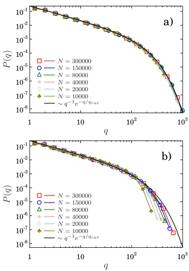
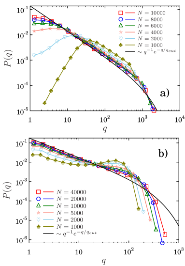
Degree distributions at equilibrium are shown in Fig. 2 for both models, for different system sizes, and fixed mean degree $\langle q\rangle=20$. In both cases, for large system sizes, the uncorrelated form of the degree distribution Eq. (13), is approached, but this convergence is much slower for the second model. The choice of mean degree was limited by the system size for which simulations run in reasonable time for the computationally more demanding model 2.

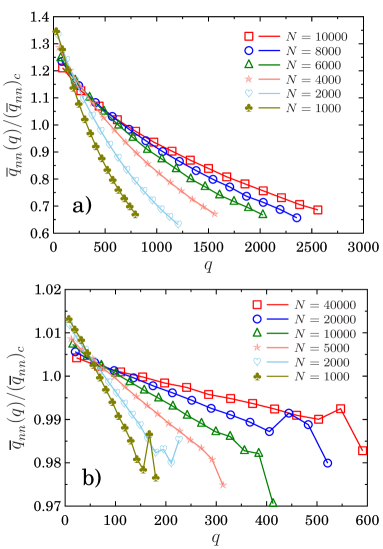
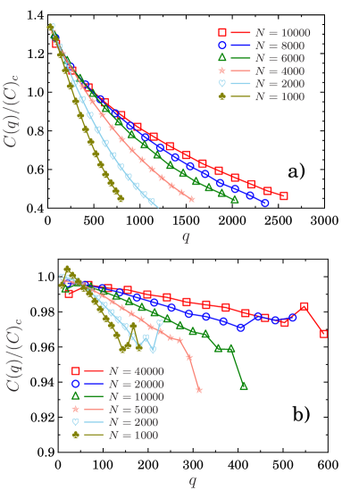
To study correlations and clustering, we measured the degree dependence of the average degree of nearest neighbours and the clustering coefficient (Figs. 3 and 4). In the plots we normalized the measured values $\overline{q}_{nn}(q)$ and $C(q)$ by the values expected in the uncorrelated case. These corresponding uncorrelated values, denoted by $(\overline{q}_{nn})_{c}$ and $(C)_{c}$, are just the values calculated in the configuration model using the same structural characteristics $N$, $\langle q\rangle$, and $\langle q^{2}\rangle$ as those obtained in the simulations:

$$(\overline{q}_{nn})_{c} = \frac{\langle q^{2}\rangle}{\langle q\rangle},$$ (23)

$$(C)_{c} = \frac{1}{N\langle q\rangle}\left\lgroup\frac{\langle q^{2}\rangle-\langle q\rangle}{\langle q\rangle}\right\rgroup^{2}.$$ (24)

Figure 3: (Color online) Degree dependence of the mean degree $\overline{q}_{nn}$ of the nearest neighbours of a node of degree $q$ for sparse equilibrium networks of mean degree $\langle q\rangle=20$ and different sizes. (a) model 1, (b) model 2. The mean degree $\overline{q}_{nn}$ is normalized by its value for the corresponding uncorrelated network.

Figure 4: (Color online) Degree dependence of the local clustering coefficient of sparse equilibrium networks of mean degree $\langle q\rangle=20$ and different sizes. (a) model 1, (b) model 2. The local clustering coefficient is normalized by its value for the corresponding uncorrelated network.

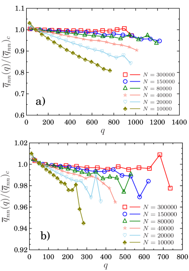
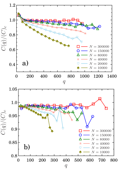
Figures 3 and 4 confirm a convergence to an uncorrelated equilibrium state for large networks. It is interesting to note that although correlations are smaller in the second model, Fig. 3(b), compared to the first one, Fig. 3(a), the degree distributions in the second model at the same sizes are still further away from the form of Eq. (13). Model 1 exhibits stronger correlations and stronger degree dependence of the local clustering coefficient (Fig. 4(a) compared with Fig. 4(b)), even though the degree distributions in model 1 (Fig. 2(a)), for the system sizes considered, already practically coincide with the uncorrelated form of Eq. (13).

III.2 Denser networks

We performed simulations of networks with higher mean node degrees, $200$ and $50$ (models 1 and 2, respectively), than in the preceeding subsection. This enabled us to observe stronger size effects in the degree distributions, Fig. 5(a), (b), than in Fig. 2 at the same network sizes. Simulations for model 2 are particularly time consuming, so the mean degree, $50$, has to be chosen smaller than $200$ for model 1. The system sizes were chosen in a way to capture a wide range of behaviors in both models, using the highest possible mean degree (limited by computational time). Figures 5(a), (b) demonstrate markedly different degree distributions for models $1$ and $2$ at low network sizes. Note that the difference is not only in a hump present in Fig. 5 (b) but this difference is well observable even in the range of small degrees. The degree-degree correlations for these networks demonstrate a stronger disassortative mixing, Fig. 6(a), (b), than for their less dense counterparts in Fig. 3(a), (b). The degree dependence of the local clustering coefficient is also more pronounced in denser networks, Fig. 7(a), (b), than in their less dense counterparts, Fig. 4(a), (b). This is especially well seen for model 1, compare respective Fig. 7(a) ($\langle q\rangle=200$) and Fig. 4(a) ($\langle q\rangle=20$).

Figure 5: (Color online) Degree distribution of denser (than in Fig. 2) equilibrium networks of different sizes. (a): $\langle q\rangle=200$, model 1; (b): $\langle q\rangle=50$, model 2.

Figure 6: (Color online) Degree dependence of the mean degree of nearest neighbours of dense equilibrium networks of varying size. (a): $\langle q\rangle=200$, model 1; (b): $\langle q\rangle=50$, model 2.

Figure 7: (Color online) Degree dependence of the clustering coefficient of dense equilibrium networks of varying size. (a): $\langle q\rangle=200$, model 1; (b): $\langle q\rangle=50$, model 2.

III.3 A real-world example

To demonstrate that degree distributions of $\gamma=1$ do exist in reality, we explore data from Facebook. The analyzed sample consists of all of the user-to-user links from the Facebook New Orleans (2009) networks V. et al. (2009). This sample has size $N=63731$ and mean degree $\langle q\rangle=25.64$. Figure 8 shows the measured Facebook degree distribution and the degree distribution from our model 1 using the same system size and mean degree. Notice the closeness of the two curves although no fitting was done. In this parameter range, the degree distribution of the model is already very close to the analytical form given by Eq. (13).

Figure 8: (Color online) Degree distribution taken from a Facebook sample, compared to the degree distribution of model 1, using the same system size and mean degree: $N=63731$ and $\langle q\rangle=25.64$.

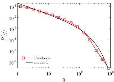
We see that the curve from our model 1 provides a good approximation of the empirical distribution. We stress that the underlying structures of the two networks are different, and so our models cannot be applied directly. Facebook is growing, and like the majority of social networks, it exhibits assortative correlations, while our equilibrium models produce disassortative ones. The Pearson correlation coefficients are $0.175$ and $-0.004$ for the Facebook sample and our model 1, respectively; with these parameters model 1 is already close to the uncorrelated sparse limit. Also, social networks have strong clustering, whereas our models have very low clustering coefficients for large systems (and clustering actually vanishes in the infinite size limit). The corresponding clustering coefficients are $0.148$ and $0.006$. Nevertheless, Fig. 8 indicates that such low exponents of the degree distribution do appear in reality. Therefore it may be useful to think outside the realm of conventional preferential attachment models in order to come closer to a full explanation of real-world network structures.

IV Discussion

Previously studied network models generating degree distributions with exponents $\gamma$ smaller than $2$ exploited a set of rather intricate mechanisms and non-trivial ideas. In particular, these included fitness models Bianconi and Barabási (2001a, b), accelerated growth, where the network becomes denser with time Dorogovtsev and Mendes (2002, 2003), aggregation processes Seyed-Allaei et al. (2006), the power of choice D’Souza et al. (2007), etc. At first sight, the two equilibrium network models that we have considered in this paper are simpler. In the infinite size limit, both these rewiring models generate uncorrelated networks with the degree distributions $P(q)\sim q^{-1}e^{-q/(\langle q\rangle\ln\langle q\rangle)}$. In finite networks, however, these models become essentially non-trivial due to constraints for rewiring which occur in this situation. We have found that these constraints lead to strong disassortative degree–degree correlations and to degree-dependent local clustering. They also markedly change the form of the degree distributions. The structural constraint is particularly strong for model 2, so the results for these two closely related models in finite systems significantly differ from each other.

Finally, we emphasize a strong difference of these rewiring models from well studied equilibrium networks based on the preferential attachment mechanism Dorogovtsev et al. (2003). While networks in the present work demonstrate a power-law degree distribution in a wide range of mean degrees, the networks from Ref. Dorogovtsev et al. (2003) are scale-free only at a critical mean degree value.

The resulting degree distributions are observable only if the mean number of connections of nodes in a network is sufficiently large. This is the case for a number of real-world networks, including social and neural networks. (The mean number of friends of adult Facebook users was already 338 in 2014 Smith and the mean number of synapses in brain neuronal networks is generally of the order of $10^{3}$ Herculano-Houzel et al. (2006); Herculano-Houzel (2012)). We suggest that our results may be useful for understanding the structural properties of networks of this kind.

References

- Newman (2001) M. E. J. Newman, “Scientific collaboration networks. I. network construction and fundamental results,” Phys. Rev. E 64, 016131 (2001).
- Liljeros et al. (2001) F. Liljeros, C. R. Edling, L. A. N. Amaral, H. E. Stanley, and Y. Åberg, “The web of human sexual contacts,” Nature 411, 907 (2001).
- Albert (2005) R. Albert, “Scale-free networks in cell biology,” J. Cell Sci. 118, 4947 (2005).
- Eguiluz et al. (2005) V. M. Eguiluz, D. R. Chialvo, G. A. Cecchi, M. Baliki, and A. V. Apkarian, “Scale-free brain functional networks,” Phys. Rev. Lett. 94, 018102 (2005).
- Faloutsos et al. (1999) M. Faloutsos, P. Faloutsos, and C. Faloutsos, “On power-law relationships of the internet topology,” in ACM SIGCOMM computer communication review, Vol. 29 (ACM, 1999) p. 251.
- Albert et al. (1999) R. Albert, H. Jeong, and A.-L. Barabási, “Internet: Diameter of the world-wide web,” Nature 401, 130 (1999).
- Barabási et al. (2000) A.-L. Barabási, R. Albert, and H. Jeong, “Scale-free characteristics of random networks: the topology of the world-wide web,” Physica A 281, 69 (2000).
- Barabási and Albert (1999) A.-L. Barabási and R. Albert, “Emergence of scaling in random networks,” Science 286, 509 (1999).
- Dorogovtsev et al. (2000) S. N. Dorogovtsev, J. F. F. Mendes, and A. N. Samukhin, “Structure of growing networks with preferential linking,” Phys. Rev. Lett. 85, 4633 (2000).
- Krapivsky et al. (2000) P. L. Krapivsky, S. Redner, and F. Leyvraz, “Connectivity of growing random networks,” Phys. Rev. Lett. 85, 4629 (2000).
- Albert and Barabási (2002) R. Albert and A.-L. Barabási, “Statistical mechanics of complex networks,” Rev. Mod. Phys. 74, 47 (2002).
- Dorogovtsev and Mendes (2002) S. N. Dorogovtsev and J. F. F. Mendes, “Evolution of networks,” Adv. Phys. 51, 1079 (2002).
- Dorogovtsev and Mendes (2003) S. N. Dorogovtsev and J. F. F. Mendes, Evolution of Networks: From Biological Nets to the Internet and WWW (Oxford University Press, Oxford, 2003).
- Dorogovtsev et al. (2003) S. N. Dorogovtsev, J. F. F. Mendes, and A. N. Samukhin, “Principles of statistical mechanics of uncorrelated random networks,” Nucl. Phys. B 666, 396 (2003).
- Adamic and Huberman (2000) L. A. Adamic and B. A. Huberman, “Power-law distribution of the world wide web,” Science 287, 2115 (2000).
- Levy and Solomon (1996) M. Levy and S. Solomon, “Power laws are logarithmic Boltzmann laws,” Int. J. Mod. Phys. C 7, 595 (1996).
- Sornette (1998) D. Sornette, “Multiplicative processes and power laws,” Phys. Rev. E 57, 4811 (1998).
- Mitzenmacher (2004) M. Mitzenmacher, “A brief history of generative models for power law and lognormal distributions,” Internet Mathematics 1, 226 (2004).
- Bianconi and Barabási (2001a) G. Bianconi and A.-L. Barabási, “Competition and multiscaling in evolving networks,” EPL (Europhys. Lett.) 54, 436 (2001a).
- Bianconi and Barabási (2001b) G. Bianconi and A.-L. Barabási, “Bose-Einstein condensation in complex networks,” Phys. Rev. Lett. 86, 5632 (2001b).
- Caldarelli et al. (2002) G. Caldarelli, A. Capocci, P. De Los Rios, and M. A. Munoz, “Scale-free networks from varying vertex intrinsic fitness,” Phys. Rev. Lett. 89, 258702 (2002).
- Kim et al. (2005) B. J. Kim, A. Trusina, P. Minnhagen, and K. Sneppen, “Self organized scale-free networks from merging and regeneration,” Eur. Phys. J. B 43, 369 (2005).
- Alava and Dorogovtsev (2005) M. J. Alava and S. N. Dorogovtsev, “Complex networks created by aggregation,” Phys. Rev. E 71, 036107 (2005).
- Seyed-Allaei et al. (2006) H. Seyed-Allaei, G. Bianconi, and M. Marsili, “Scale-free networks with an exponent less than two,” Phys. Rev. E 73, 046113 (2006).
- Valverde et al. (2002) S. Valverde, R. Ferrer i Cancho, and R. V. Solé, “Scale-free networks from optimal design,” EPL (Europhysics Letters) 60, 512 (2002).
- D’Souza et al. (2007) R. M. D’Souza, P. L. Krapivsky, and C. Moore, “The power of choice in growing trees,” Eur. Phys. J. B 59, 535 (2007).
- Burda et al. (2001) Z. Burda, J. D. Correia, and A. Krzywicki, “Statistical ensemble of scale-free random graphs,” Phys. Rev. E 64, 046118 (2001).
- Burda and Krzywicki (2003) Z. Burda and A. Krzywicki, “Uncorrelated random networks,” Phys. Rev. E 67, 046118 (2003).
- Krioukov et al. (2010) D. Krioukov, F. Papadopoulos, M. Kitsak, A. Vahdat, and M. Boguñá, “Hyperbolic geometry of complex networks,” Phys. Rev. E 82, 036106 (2010).
- Papadopoulos et al. (2012) F. Papadopoulos, M. Kitsak, M. Á. Serrano, M. Boguñá, and D. Krioukov, “Popularity versus similarity in growing networks,” Nature 489, 537 (2012).
- Zuev et al. (2016) K. Zuev, F. Papadopoulos, and D. Krioukov, “Hamiltonian dynamics of preferential attachment,” J. Phys. A 49, 105001 (2016).
- Colomer-de Simon and Boguná (2012) P. Colomer-de Simon and M. Boguná, “Clustering of random scale-free networks,” Phys. Rev. E 86, 026120 (2012).
- Anand et al. (2014) K. Anand, D. Krioukov, and G. Bianconi, “Entropy distribution and condensation in random networks with a given degree distribution,” Phys. Rev. E 89, 062807 (2014).
- Pietronero et al. (2001) L. Pietronero, E. Tosatti, V. Tosatti, and A. Vespignani, “Explaining the uneven distribution of numbers in nature: the laws of Benford and Zipf,” Physica A 293, 297 (2001).
- V. et al. (2009) Bimal V., Alan M., Meeyoung C., and Krishna P. G., “On the evolution of user interaction in Facebook,” in Proceedings of the 2nd ACM SIGCOMM Workshop on Social Networks (WOSN’09) (2009).
- (36) A. Smith, “6 new facts about Facebook,” Pew Research Center, http://www.pewresearch.org/fact-tank/2014/02/03/6-new-facts-about-facebook.
- Herculano-Houzel et al. (2006) S. Herculano-Houzel, B. Mota, and R. Lent, “Cellular scaling rules for rodent brains,” Proc. Natl. Acad. Sci. USA 103, 12138 (2006).
- Herculano-Houzel (2012) S. Herculano-Houzel, “The remarkable, yet not extraordinary, human brain as a scaled-up primate brain and its associated cost,” Proc. Natl. Acad. Sci. USA 109, 10661 (2012).