Network Densification in 5G: From the Short-Range Communications Perspective

Abstract

Besides advanced telecommunications techniques, the most prominent evolution of wireless networks is the densification of network deployment. In particular, the increasing access points/users density and reduced cell size significantly enhance spatial reuse, thereby improving network capacity. Nevertheless, does network ultra-densification and over-deployment always boost the performance of wireless networks? Since the distance from transmitters to receivers is greatly reduced in dense networks, signal is more likely to be propagated from long- to short-range region. Without considering short-range propagation features, conventional understanding of the impact of network densification becomes doubtful. With this regard, it is imperative to reconsider the pros and cons brought by network densification. In this article, we first discuss the short-range propagation features in densely deployed network and verify through experimental results the validity of the proposed short-range propagation model. Considering short-range propagation, we further explore the fundamental impact of network densification on network capacity, aided by which a concrete interpretation of ultra-densification is presented from the network capacity perspective. Meanwhile, as short-range propagation makes interference more complicated and difficult to handle, we discuss possible approaches to further enhance network capacity in ultra-dense wireless networks. Moreover, key challenges are presented to suggest future directions.

I Introduction

Instead of the enhancement of radio access networks (RANs), the future wireless networks are more likely to act as a mixture of various types of RANs, e.g., macro-cell base stations (BSs), femto-cell BSs, pico-cell BSs and WiFi access points (APs), etc. By 2030, the targets are to support ubiquitous device connectivity and expand network capacity, including 100 billion device connections, 20000$\times$ mobile data traffic and 1000$\times$ user experienced data rate, etc., compared to 2010 [1]. The requirements are even more critical for popular scenarios. For instance, tens of Tbps/$\mathrm{km}^{2}$ is required in the office, 1 million connections/$\mathrm{km}^{2}$ is required at densely populated areas such as stadium and open gathering, and super high density of over 6 persons/$\mathrm{m}^{2}$ is to be supported in subways. Among the appealing approaches to realize the ambitious goals, network densification is shown to be the most promising one, which has improved network capacity by 2700 folds from 1950 to 2000 [2]. The principle of network densification is to deploy BSs/APs with smaller coverage and enables local spectrum reuse. In consequence, users can be served with shorter transmission links, thereby fully exploiting spatial and spectral resources.

However, does aggressively deploying more BSs and devices always improve the system performance? As network densification significantly reduces transmission distance and enables proximity communication, the signal propagation may transit from long- to short-range propagation. For instance, as shown in Table II, if the BS density is increased from 1 $\mathrm{BS}/\mathrm{km}^{2}$ to 100 $\mathrm{BS}/\mathrm{km}^{2}$, the average transmission link length is reduced 10 folds from 500 m to 50 m, which makes a larger proportion of downlink users located within the short-range propagation distance. Meanwhile, the application of device-to-device (D2D) communications allows direct local transmission of nearby users to bypass centralized BSs, which greatly shortens the distance between transmitters (Tx’s) and the potential receivers (Rx’s) as well. As will be discussed later, signal propagation features are different within long- and short-range regions, e.g., signal strength decays moderately with transmission distance in short-range regions, while decays more quickly in long-range regions. Accordingly, signal attenuation features have to be modeled differently. However, in traditional wireless communications system, the performance evaluation and protocol design are basically based on the assumption of long-range transmission. Therefore, the impact of network densification and short-range transmission on network performance remains to be explored.

Recently, the research of densely deployed wireless networks has gained great attention from both academia and industries, including architecture development [3, 4], analytical studies [5, 6] and protocol design [7]. Remarkably, a user-centric architecture has been presented for ultra-dense networks (UDN) [4], under which functions such as mobility management, resource management and interference management, can be co-designed and jointly optimized. Meanwhile, to comprehensively understand the merits and limits brought by network densification, authors study the network capacity scaling law in downlink cellular network[5, 6]. Wherein, the impact of both line-of-sight (LoS) and non-LoS (NLoS) transmissions has been fully explored. Depending on parameters, it is shown that the spatial throughput, which is an indicator of network capacity, scales slowly and even diminishes to be zero when BS density is sufficiently large [5]. The above results indicate that network densification may be beneficial, while network ultra-densification would lose the merits of network capacity enhancement when spatial resources are fully exhausted. Nevertheless, despite the progress achieved by recent research, there is still no consensus on how dense is ultra-dense in wireless networks. More importantly, the available study fails to capture the influence of short-range transmissions in UDN, which makes the existing results dubious and doubtful.

With this regard, we intend to characterize ultra-densification for wireless networks by fully exploring short-range propagation features. To this end, we first provide answers to the following two questions: 1) how to characterize short-range propagation features and 2) how short-range propagation influences the performance of wireless networks in terms of spatial throughput. Aided by the spatial throughput scaling law, we then concretely reveal how dense is ultra-dense in wireless networks. To combat interference and further enhance the system performance in UDN, we overview the state-of-the-art technologies like interference management, non-orthogonal multiple access (NOMA), and millimeter-wave (mm-Wave) communications, and key challenges to facilitate them in UDN are highlighted as well.

The rest of this article is organized as follows. We first discuss signal propagation features within short distance via experimental results. Then, the interpretation of ultra-densification is presented from the spatial throughput scaling perspective. Following that, the detail of the possible approaches to further enhancing the capacity in UDN is discussed, and open challenges brought by ultra-densification are provided as well. Finally, conclusion remarks are drawn.

II Short-Range Propagation in UDN

Avg. of link length $d$ (m)	BS density $\left(\mathrm{BS}/\mathrm{km}^{2}\right)$	$\mathtt{P}\left(d<50\>\mathrm{m}\right)$	$\mathtt{P}\left(d<20\>\mathrm{m}\right)$	$\mathtt{P}\left(d<10\>\mathrm{m}\right)$	$\mathtt{P}\left(d<1\>\mathrm{m}\right)$
500	1	0.78%	0.13%	0.03%	$3.1\times 10^{-6}$
100	25	17.8%	3.1%	0.78%	0.01%
50	100	54.4%	11.8%	3.1%	0.03%
10	2500	$\approx$100%	95.7%	54.4%	0.8%
5	10000	$\approx$100%	$\approx$100%	95.7%	3.1%

Table I. The probability that cellular transmission occur within different distances. The above statisitics are obtained via simulations provided that users are connected to the geometrically nearest BSs.

It is evident that network densification would push Tx’s and Rx’s closer to each other. Taking cellular networks as an example, when small cells are deployed for ubiquitous and seamless coverage, the transmission distance from users to small cell BSs is greatly reduced from hundreds of meters (macro cell case) to tens of meters. In the upcoming fifth generation (5G) wireless networks, small cell BSs of plug-and-play features would be deployed anywhere (on the tables or the roof of a room) and accordingly the transmissions would occur within much shorter distance (e.g., up to 10m). For instance, when the nearest neighbor connectivity rule is adopted, i.e., users are supposed to connect to the geometrically closest BSs, the probabilities that transmission occurs within different regions are shown in Table I. It is observed that the probability that transmission occurs within 20m raises 91 folds from 0.13% to 11.8% when BS density increases from 1 $\mathrm{BS}/\mathrm{km}^{2}$ to 100 $\mathrm{BS}/\mathrm{km}^{2}$. If BS density further increases from 1 $\mathrm{BS}/\mathrm{km}^{2}$ to 2500 $\mathrm{BS}/\mathrm{km}^{2}$, this probability astonishingly raises 750 folds from 0.13% to 95.7%. This is especially true for scenarios like offices and dining halls, etc. For more crowded places, such as stadiums, more dense BS deployment is required such that transmission distance is further reduced. In addition, we see from Table I that almost all the transmissions occur within 10 m when the BS density reaches 10000 $\mathrm{BS}/\mathrm{km}^{2}$.

It is worth noting that signal propagation features within short distance, e.g., up to 10m, significantly differ from those in the long distance, e.g., larger than 50m. Even when they are located in proximity and LOS path exists between them, signal propagations may be still different. For instance, when Tx’s are dozens of meters apart from Rx’s, the LOS component of signals dominates the NLOS component and accordingly, the wireless channels between them are likely to experience Rician fading. In contrast, when Tx’s and Rx’s are in close proximity, the LOS and NLOS components become less distinguishable. As will be shown later, it is more likely that the channel between Tx’s and Rx’s is a Rayleigh fading channel.

According to the above discussion, to better understand the impact of network densification, it is essential to figure out signal propagation features over different propagation distance. To shed light on this, we discuss short-range propagation features via experimental results in the following.

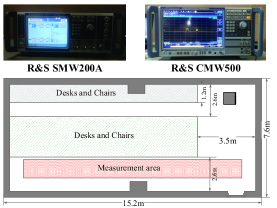
(a) Experimental scenarios.

(b) Experimental setups.

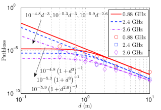
(c) Experimental and fitting results.

Figure 1: Experimental results of received signal power for short-range transmission. In (b), markers denote the experimental results and lines denote the fitting results. Transmit power of the signal generator is set to be 0 dBmW.

II-A Experimental Results of Short-Range Signal Propagation

In this part, we use experimental results to illustrate how pathloss varies with transmission distance $d$ especially when $d$ is small. The measurement is conducted in the meeting room of size 15.2m$\times$7.6m, as shown in Fig. 1a. Meanwhile, it can be seen in Fig. 1b that the Tx omnidirectional antenna is connected to a Rohde & Schwarz SMBV200A Vector Signal Generator and the Rx omnidirectional antenna is connected to a Rohde & Schwarz CMW500 Wideband Radio Communication Tester. Signal carrier frequencies are set to be 0.88GHz, 2.4GHz and 2.6GHz, respectively. Signal power decay within short distance can be reflected using the results in Fig. 1c.

Fig. 1c shows the channel power gain as a function of transmission distance $d$, where BPM and unbounded pathloss model (UPM) $d^{-\alpha}$ [8, 5, 6] are applied to derive the fitting results. It can be seen that the gaps between experimental and fitting results under UPM are large when over small transmission distance. This is due to the singularity of UPM at $d=0$ m and the fact that the UPM would artificially make the received signal power greater than the transmitted signal power when $d\in\left[0,1\right]$m. Instead, the channel power gain is shown to be accurately modeled using BPM even when $d$ is small. Therefore, the experimental results are sufficient to indicate the rationality of using BPM to model pathloss especially within short-range regions.

In addition to the above discussion, how to characterize short-range propagation features would significantly influence the performance evaluation and protocol design in UDN. In particular, under BPM, we have found that network ultra-densification would eventually drain the spatial reuse and render network capacity diminishing to be zero. As will be discussed later, this differs from the results in [5, 6] that spatial throughput scales linearly/sublinearly with BS density under UPM.

II-B From Long-range Propagation to Short-range Propagation

The above experimental results indicate that the signal power would decay slowly with distance within short range. In constrast, it is evident that signal power may decay rapidly with distance when long-range transmission occur. For this reason, to model signal propagation in UDN, it is crucial to accurately capture the characteristics of channel gain within different propagation regions. Combining the available results in literature[5, 9, 10], we propose to use multi-slope BPM

$$g_{N}^{\mathrm{B}}\left(\left\{\alpha_{n}\right\}_{n=0}^{n=N-1};d\right)=\eta_{n}\left(1+d^{\alpha_{n}}\right)^{-1},\>R_{n}<d\leq R_{n+1},$$ (1)

where $d$ denotes the distance from Tx to Rx, $R_{n}$ denotes critical distance and $\alpha_{n}$ denotes the pathloss exponent for $R_{n}<d\leq R_{n+1}$. Meanwhile, $\eta_{0}=1$ and $\eta_{n}=\underset{i=1}{\overset{n}{\prod}}\frac{1+R_{i}^{\alpha_{i}}}{1+R_{i}^{\alpha_{i-1}}}$ are defined to maintain continuity of (1). As signals are attenuated faster in larger distance , $\alpha_{n}<\alpha_{n+1}$ holds. Besides, the multi-slope model in (1) can be applied into different scenarios as well.

1) Sparse outdoor scenarios: When $N=1$, (1) degenerates into the single-slope BPM, where one pathloss exponent is used to characterize the power decay rate in the free space. Therefore, the model is suitable for the sparse scenarios, where Tx’s are basically located apart from Rx’s.

2) Dense outdoor scenarios: When $N=2$, (1) degenerates into the dual-slope BPM, where two pathloss exponents are used within and out of the critical distance. Therefore, this model can be applied in dense outdoor scenarios such as stadium and open gatherings, where Tx’s and Rx’s are located close to each other and there are signal LoS and reflected components.

3) Dense indoor scenarios: When $N>2$, multiple pathloss exponents are used to capture the discrepant power decay rates within different transmission distances. This is especially true for the indoor scenarios, where signals from different floors and regions may be attenuated with different rates.

II-C Spatial Correlation of Wireless Channels

Besides short-range propagation of discrepant features, another dominant property caused by network densification is the spatial correlation of wireless channels. In general, the LOS and reflected components between Tx and Rx contributes to the variation of wireless channels. When Tx’s (or Rx’s) are in close proximity in UDN, they may have almost identical LOS and reflected component, and consequently, the wireless channels between them are more likely to be spatially dependent. Taking uplink transmissions for example, assuming the users located in proximity (several wavelength apart) are associated with different small cell BSs, the generated desired and interfering signals over these channels are likely to be correlated. More specifically, if the desired signals are of great attenuation, the interfering signals from nearby users associated with other BSs are likely to be in deep fading as well.

On the one hand, the performance evaluation of UDN in most of the existing literatures is based on the premise that wireless channels are uncorrelated. Therefore, the performance of UDN may be over-estimated and is to be further investigated. On the other hand, channel independence is the pre-assumption of most multi-antenna communications techniques, such as coordinated multipoint (CoMP) and interference alignment (IA), etc. For this reason, great challenges are posed towards the design and application of these techniques, the detail of which will be discussed later.

Figure 2: . The CDF of interference under UPM and BPM in sparse and dense deployment scenarios. The tested user is located at the center of a square with side length 1000m. A full spectrum reuse policy is adopted by the interferers, which are randomly located within the scenario. Channel power gain consists of pathloss and small scale fading. In particular, dual-slope UPM and BPM, with $\alpha_{0}=2$, $\alpha_{1}=4$ and $R_{1}=10$m, serve as the pathloss models. Denoting $d_{ij}$ as the distance from $\mathrm{BS}_{i}$ and $\mathrm{BS}_{j}$, $\exp\left(-d_{ij}/D_{\mathrm{C}}\right)$ is applied to quantify the correlation coefficient between $\mathrm{BS}_{i}$ and $\mathrm{BS}_{j}$, where $D_{\mathrm{C}}$ denotes the decorrelation distance. In simulations, the transmit power of each interferer is set to be 23dBmW and the noise power is -110 dBmW.

III Interpretation of Network Densification: From the Spatial Throughput Perspective

Although ultra-densification is a growing trend for the future wireless networks, there is still no consensus on how dense is ultra-dense. To answer the question, in this part, we show some of our recent results on the spatial throughput of wireless networks and give the interpretation of ultra-densification from the perspective of spatial throughput scaling law.

We define spatial throughput as follows:

$$\mathcal{ST} =\mu\mathbb{P}\left(\mathtt{SINR}>\text{$\tau$}\right)\log\left(1+\tau\right),\>\left[\mathrm{bits}/\left(\mathrm{s\cdot Hz\cdot m^{2}}\right)\right]$$ (2)

where $\mu$ denotes the density of active links, $\tau$ denotes the signal-to-noise-and-interference ratio (SINR) threshold and $\mathbb{P}\left(\mathtt{SINR}>\text{$\tau$}\right)$ denotes the success probability of data transmissions.

Intuitively, interference may degrade the SINR and the corresponding transmission success probability especially when $\mu$ is large, thereby serving as a limiting factor to spatial throughput. Meanwhile, considering short-range propagation, the interference distribution becomes complicated. Therefore, we first look into the features of interference in wireless networks by comparing sparse and dense scenarios.

III-A Interference Distribution in Wireless Networks

Fig. 2 shows the cumulative distribution function (CDF) of interference levels (in dBm) suffered by a tested user, which is located at the center of the testing scenario. It is shown from Fig. a that the interference CDF is almost identical under …. when … However, when the BS density grows, we notice that the difference in the interference distribution is evident under different channel models. Notably, the CDF experiences a heavy tail under UPM, which is physically unreasonbly. This is due to the singularity of UPM when the transmission distance approaches zero. For this reason, it is no longer reasonable to use UPM to model pathloss under dense deployment. Besides, to highlight the impact of channel correlation on the interference distribution, we compare the CDFs of interference levels with and without channel correlations under BPM in Fig. b. Likewise, it can be seen that the influence of channel correlation on interference distribution is negligible when interferers are sparsely distributed. Nevertheless, the influence becomes evident when interferers are fully densified. Specifically, we can see from Fig. b that channel correlation would result in the degradation of interference levels. Therefore, without considering channel correlation in UDN, the performance of wireless networks would be greatly over-estimated, the details of which are illustrated in the following.

III-B Interpret Ultra-Densification From Spatial Throughput Perspective

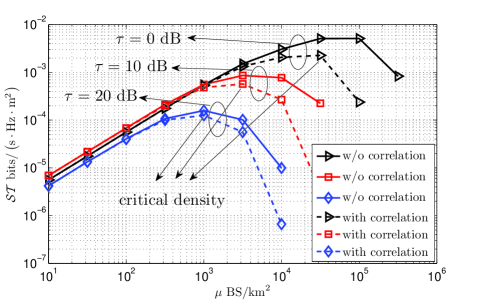
Figure 3: Spatial throughput scaling with BS density $\mu$ under different decoding threshold $\tau$ in downlink cellular networks. Single-antenna downlink users are connected to the geometrically nearest single-antenna BSs, both of which are assumed to be distributed according to Poisson point processes. One user is served by one BS and no interference management techniques are applied. Meanwhile, user density is much larger than the BS density to guarantee that each BS is associated with at least one user. Channel correlation coefficient is quatified by $K_{i,j}=\exp\left(-d_{i,j}/D_{\mathrm{C}}\right)$, where $d_{i,j}$ denote the distance from $\mathrm{BS}_{i}$ to $\mathrm{BS}_{j}$ and $D_{\mathrm{C}}$ denotes the decorrelation distance. Dual-slope BPM, i.e., $N=2$ in (1), serves as the pathloss model. System parameters are set as $\alpha_{0}=2$, $\alpha_{1}=4$, $R_{\mathrm{C}}=10$m and $D_{\mathrm{C}}=10$m.

Based on (2), we investigate the spatial throughput of an outdoor downlink cellular network. Specifically, we plot the spatial throughput defined in (2) as a function of BS density under different decoding threshold $\tau$ in Fig. 3. To highlight the impact of channel correlation on the spatial throughput, we compare the cases with and without considering channel correlation. It is evident that the gaps between the two cases are enlarged as the network is densified. This indicates that the network performance is increasingly over-estimated when channel correlation is not taken into account. Moreover, it is observed in Fig. 3 that the spatial throughput derived under BPM scales with rate $\mu e^{-\kappa\mu}$, i.e., first increases with $\mu$ and then decreases with $\mu$ [12]. Note that $\kappa$ is a function of system parameters. In other words, network densification would degrade spatial throughput when BS density is sufficiently large. For this reason, we characterize ultra-densification in terms of the spatial throughput scaling behavior.

Ultra-densification: Wireless networks are considered ultra-dense when the network density is larger than the critical density, beyond which system spatial throughput begins to decay. The network density has different interpretations in different network architectures. For instance, it refers to BS density in cellular uplink/downlink networks, while refers to density of activated Tx’s in ad hoc/D2D networks.

SINR Threshold	$\mu_{1}^{*}\>\left(\mathrm{BS}/\mathrm{km}^{2}\right)$	$\mu_{2}^{*}\>\left(\mathrm{BS}/\mathrm{km}^{2}\right)$	$\mu_{3}^{*}\>\left(\mathrm{BS}/\mathrm{km}^{2}\right)$
$\tau$ $\left(\mathrm{dB}\right)$	$\alpha_{0}=2$	$\alpha_{0}=2$	$\alpha_{0}=2$
	$\alpha_{1}=3$	$\alpha_{1}=3.5$	$\alpha_{1}=4$
0	2.0$\times 10^{5}$	2.51$\times 10^{5}$	3.16$\times 10^{5}$
5	7.94$\times 10^{4}$	1.26$\times 10^{5}$	1.59$\times 10^{5}$
10	3.16$\times 10^{4}$	6.31$\times 10^{4}$	7.94$\times 10^{4}$
15	1.58$\times 10^{4}$	3.16$\times 10^{4}$	5.01$\times 10^{4}$
20	6.3$\times 10^{3}$	1.58$\times 10^{4}$	2.51$\times 10^{4}$

Table II. Critical density $\mu^{*}$ for empirical pathloss exponent settings [13]. Note that dual-slope BPM is applied as the pathloss model, which is obtained by setting $N=2$ in (1).

Table II shows the critical densities under typical system settings, which are derived by making an extension of the results in [12]. Under the dual-slope BPM with $\alpha_{1}=3.5$, we observe that up to 6.31$\times 10^{4}$ BSs can be deployed per square kilometer to maximize the spatial throughput when $\tau=10\>\mathrm{dB}$. Otherwise, if more BSs are deployed, the detriment of resulting inter-cell interference overwhelms the benefits of spatial reuse, which degrades spatial throughput. In this case, provided that 1 million connections/$\mathrm{km}^{2}$ are to be supported in the places such as open gathering [1], almost 16 connections are served by each BS. Meanwhile, it is also observed that if users demand for higher transmission rate or equivalently greater SINR threshold, the critical BS density is reduced. This is because the transmission with higher rate is vulnerable and more likely to be interrupted by inter-cell interference. In addition, Table II indicates that larger pathloss exponents lead to larger critical densities. In particular, the critical density increases to 2.51$\times 10^{4}$ $\mathrm{BS}/\mathrm{km}^{2}$ under the dual-slope BPM with $\alpha_{1}=4$ and $\tau=20\>\mathrm{dB}$. The reason is that interference would decay more quickly with distance under larger pathloss exponents. As a result, its influence on spatial throughput is weakened. Note that the empirical pathloss exponents are basically large in urban areas, where the building blocks either form a regular Manhattan type of grid or have more irregular locations [13].

The above results also confirm the importance of applying multi-slope BPM to model the pathloss in ultra-dense scenarios. Despite capturing the different power decay rates over different distances, multi-slope UPM fails to capture the power loss within short-range regions. This makes the increase of aggregate interference power be counter-balanced by the increase of the desired signal power. Consequently, the successful probability in (2) is over-estimated and spatial throughput linearly/sublinearly increases with the BS density $\mu$. Instead, the multi-slope BPM is capable of characterizing moderate power decay within short-range region, which is consistent with practice (see Fig. 1). Under BPM, the spatial throughput is shown to be eventually degraded by the over-deployment of BSs. Therefore, multi-slope BPM could serve as a reasonable pathloss model especially in UDN.

Aided by the interpretation of ultra-densification in Fig. 3, we have been fully aware of the fact that over-deployment of BSs/APs and over-activation of devices indeed degenerate the performance of wireless networks. Then, the following question comes up: how to breakthrough the limitation of network densification and further enhance the capacity of UDN? The detail will be discussed in the following section.

IV Possible Approaches and Challenges to Improve Capacity in UDN

For capacity enhancement, a number of state-of-the-art techniques can be applied. However, challenges exist as well in practical implementations due to the channel and interference characteristics in UDN.

IV-A Interference Management

Since severe and complicated interference is the key factor to bottleneck the capacity in UDN, interference management techniques are of the greatest potential to combat interference and improve network capacity. Interference cancellation and interference coordination are two prevalent interference management techniques. Applying interference cancellation, interference signals are rebuilt, decoded and finally successively or parallelly removed from the aliasing signals until the desired signal is retrieved. Decoding interference signals requires that interference signals are of great disparity. For interference coordination, with the aid of multi-antenna technologies, desired signal and interference signals are forced to be spatially orthogonal at Rx’s via jointly designing precoders by multiple Tx’s (or both Tx’s and Rx’s). Channel independence is the premise for joint precoder design. However, the interference and channel features in UDN greatly degrade the performance of interference cancellation and interference coordination. On the one hand, interference signals basically stem from the interferers, which are geometrically close to the intended Rx in dense scenarios. Accordingly, the interference levels become less divergent. On the other hand, as discussed earlier, network densification makes the channels of transmission pairs in close proximity become spatially correlated as well. This may directly ruin the merits brought by multi-antenna based interference management techniques.

IV-B Non-Orthogonal Multiple Access

NOMA also serves as a promising method to improve user connectivity and network capacity by fully multiplexing available spectrum resources via non-orthogonal spectrum sharing [14]. The key to NOMA is to cancel the proactively introduced spectrum-domain interference in other domains. For instance, the power domain based NOMA (PD-NOMA) and sparse code multiple access (SCMA) exploit the degree of freedom in power domain and code domain, respectively. However, as discussed earlier, as interference cancellation would lose the merit due to the narrowed interference levels, the performance of NOMA is degrades in UDN. Worsestill, NOMA is basically co-designed with resource allocation. To enable effcient resource allocation, accurate overhead for channel estimation and information exchange is required. Yet, the overhead caused by network over-deployment would be massive and further increase with the user density, which in turn ruins the potential benefits of NOMA. Hence, how to design scalable NOMA remains to be an open issue in UDN.

IV-C Millimeter-Wave Communications

The reduced transmission distance makes it possible to apply millimeter-wave (mm-Wave) communications in UDN [15]. Under mm-Wave bands over 30-100GHz, higher data rates and larger network capacity can be readily guaranteed. Moreover, interference signals are more rapidly decays with transmission distance over higher frequency bands, which ensures lower interference levels in mm-Wave communications. Even when interferers are in close proximity, interference could be spatially avoided with the aid of directional antennas. Despite the benefits, antenna directivity feature would result in serious problems as well. Especially, the antenna directions, which depend on the relative locations of Tx’s and the intended Rx’s, have to adjust dynamically when Tx’s or Rx’s are on the move. On the one hand, acquiring instantaneous location information in UDN is a waste of overhead, which limits the implementation of mm-Wave communications. On the other hand, the adjustment of antenna directions among adjecent transmission pairs would make the transmission pairs, which are interference-free, potentially interfere with each other. Consequently, how to design mm-Wave techniques under the above considerations is challenging.

V Conclusion Remarks

As an inevitable tendency in future wireless networks, network densification significantly reduces transmission distance and make signal propagation transit from long- to short-range propagation. In this article, we discuss the impact of short-range propagation on the wireless network performance, especially considering densely deployed scenarios. Remarkably, we found that network densification would eventually drain the spatial resources and degrade network performance when network density exceeds a critical density. More importantly, aided by the critical density, we interpret network ultra-densification from the perspective of spatial throughput scaling law. The result serves as a guidance for network deployment, as it indicates under what circumstances deploying more BSs/APs is beneficial to enhancing network capacity. In summary, this article has merely shed light on a drop in the bucket of UDN. It is imperative to fully understand and exploit the inherent features of UDN, thereby achieving the aggressive goals of future wireless networks.

References

- [1] IMT-2020 (5G) Promotion Group, “5G vision and requirements,” Tech. Rep., Dec. 2015. [Online]. Available: http://www.imt-2020.org.cn/en/documents/download/3
- [2] W. Webb, ArrayComm. London, U.K.: Ofcom, 2007.
- [3] P. K. Agyapong, M. Iwamura, D. Staehle, W. Kiess, and A. Benjebbour, “Design considerations for a 5G network architecture,” IEEE Commun. Mag., vol. 52, no. 11, pp. 65–75, Nov. 2014.
- [4] S. Chen, F. Qin, B. Hu, X. Li, and Z. Chen, “User-centric ultra-dense networks for 5G: challenges, methodologies, and directions,” IEEE Wireless Commun., vol. 23, no. 2, pp. 78–85, April 2016.
- [5] X. Zhang and J. G. Andrews, “Downlink cellular network analysis with multi-slope path loss models,” IEEE Trans. Commun., vol. 63, no. 5, pp. 1881–1894, May 2015.
- [6] M. Ding, P. Wang, D. Lopez-Perez, G. Mao, and Z. Lin, “Performance impact of LoS and NLoS transmissions in dense cellular networks,” IEEE Trans. Wireless Commun., vol. 15, no. 3, pp. 2365–2380, Mar. 2016.
- [7] Z. Zhou, M. Dong, K. Ota, and Z. Chang, “Energy-efficient context-aware matching for resource allocation in ultra-dense small cells,” IEEE Access, vol. 3, pp. 1849–1860, Sep. 2015.
- [8] H. S. Dhillon, R. K. Ganti, F. Baccelli, and J. G. Andrews, “Modeling and analysis of K-Tier downlink heterogeneous cellular networks,” IEEE J. Sel. Areas Commun., vol. 30, no. 3, pp. 550–560, Apr. 2012.
- [9] H. Inaltekin, M. Chiang, H. V. Poor, and S. B. Wicker, “On unbounded path-loss models: effects of singularity on wireless network performance,” IEEE J. Sel. Areas Commun., vol. 27, no. 7, pp. 1078–1092, Sep. 2009.
- [10] R. K. Ganti and M. Haenggi, “Interference and outage in clustered wireless ad hoc networks,” IEEE Trans. Inf. Theory, vol. 55, no. 9, pp. 4067–4086, Sep. 2009.
- [11] H. Inaltekin, “Gaussian approximation for the wireless multi-access interference distribution,” IEEE Trans. Signal Process., vol. 60, no. 11, pp. 6114–6120, Nov. 2012.
- [12] J. Liu, M. Sheng, L. Liu, and J. Li, “Effect of densification on cellular network performance with bounded pathloss model,” IEEE Commun. Lett., vol. 21, no. 2, pp. 346–349, 2017.
- [13] P. Kyösti, J. Meinilä, L. Hentilä, X. Zhao, T. Jämsä, C. Schneider, M. Narandzic, M. Milojevic, A. Hong, J. Ylitalo et al., “Winner II channel models,” WINER II Public Deliverable, pp. 42–44, 2007.
- [14] L. Dai, B. Wang, Y. Yuan, S. Han, C. l. I, and Z. Wang, “Non-orthogonal multiple access for 5G: solutions, challenges, opportunities, and future research trends,” IEEE Commun. Mag., vol. 53, no. 9, pp. 74–81, Sept. 2015.
- [15] R. Baldemair, T. Irnich, K. Balachandran, E. Dahlman, G. Mildh, Y. Selén, S. Parkvall, M. Meyer, and A. Osseiran, “Ultra-dense networks in millimeter-wave frequencies,” IEEE Commun. Mag., vol. 53, no. 1, pp. 202–208, Jan. 2015.