Realization of anomalous multiferroicity in free-standing graphene with magnetic adatoms

Abstract

It is generally believed that free-standing graphene does not demonstrate any ferroic properties. In the present work we revise this statement and show that single graphene sheet with a pair of magnetic adatoms can be driven into ferroelectric (FE) and multiferroic (MF) phases by tuning the Dirac cones slope. The transition into the FE phase occurs gradually, but an anomalous MF phase appears abruptly by means of a Quantum Phase Transition. Our findings suggest that such features should exist in graphene recently investigated by Scanning Tunneling Microscopy (Science 352, 437 (2016)).

I Introduction

Multiferroic (MF) materials, i.e., compounds where ferroelectricity and magnetic ordering coexist, have been recognized as systems with large applications in the modern device industryKhomskii ; Eerenstein . Nowadays, it is well-known that the mechanisms behind the multiferroic behavior are not universal and thus often material specificReview1 ; Review2 . The origin of the MF response is thus a puzzling issue which attracts the attention of researchers working in the domains of both condensed matter physics and materials science. Prominent examples where multiferroicity can be found include frustrated magnetsKimura ; Hur ; Cheong ; systems involving the Dzyaloshinskii-Moriya interaction as observed in manganites with spiral spin-orderFiebig ; Cheong , in which the concomitant formation of electric-dipoles and long-range magnetic ordering takes place; the recently reported 2D systems with “Mexican-hat” type band-structureMexicanH ; incommensurate states with broken lattice inversion symmetryFeTe ; and molecular conductors, where the MF behavior is linked to electron-electron correlationsFSalts ; Mariano .

In this work, we investigate the perspective of using single graphene monolayer for achievement of MF behavior. It is well known that free-standing graphene is not suitable for this purposeDresselhaus ; CNeto ; BUchoa , thus we propose to add a pair of collinear magnetic adatoms to it situated from different sides of the sheet as shown at Fig.1. The onset of the MF phase is achieved by tuning the slope of the Dirac cones, which breaks adatom-graphene sublattice symmetry at some critical point and drives the system towards a Quantum Phase Transition (QPT) from the ferroelectric (FE) phase to the MF.

This multiferroicity is anomalous, once this phase is preceded by a purely FE phase just with charge ordering where the local magnetic moments of the adatoms are quenched, in opposite to the conventional MF behavior, characterized by ordering parameters of ferroelectric and magnetic-type emerging concomitantlyReview1 ; Review2 and also due to the lack of conjugate fields (electric and magnetic) as tuning parameters of the phase transition. Here, we show that both can be replaced by just a single tuning parameter, which is established by the Fano factor $q_{0}$ of interference responsible for changing the Dirac cones slope. In this way, standard hysteresis loops depending upon the conjugate fields for identifying ferroelectricity and the single-phase multiferroics are not required within our framework.

Figure 1: (Color online) MF phase of two energetically different magnetic adatoms ($\Delta\mathcal{E}$) collinear to a carbon: distinct charge accumulations $\delta^{+}$ and $\delta^{-}$ together with a net magnetization (vertical arrows) can split over these adatoms. In this system, a QPT modifies abruptly the FE phase into the MF, due to the increasing of the Fano factor $q_{0}>q_{c}$ above the critical point, via the tuning of the Dirac cones slope (the Fermi velocity $v_{F}$).

II The model

To give theoretical description of the system under consideration, the Anderson-type HamiltonianBUchoa ; Anderson can be proposed:

$$\mathcal{H}^{\text{2D}} =-t\sum_{\mathbb{k}\sigma}[\phi({\mathbb{k}})a_{\mathbb{k}\sigma}^{\dagger}b_{\mathbb{k}\sigma}+\text{H.c.}]+\sum_{l\sigma}\mathcal{E}_{l}d_{l\sigma}^{\dagger}d_{l\sigma}$$

$$+[\mathcal{V}_{0}^{A}\sum_{\mathbb{k}l\sigma}(a_{\mathbb{k}\sigma}^{\dagger}+\frac{t}{D}q_{0}\phi({\mathbb{k}})b_{\mathbb{k}\sigma}^{\dagger})d_{l\sigma}+\text{H.c.}]$$

$$+\sum_{l}\mathcal{U}n_{l\uparrow}n_{l\downarrow.}$$ (1)

In this expression, $D$ is the bandwidth, $\phi({\mathbb{k}})=\sum_{i=1}^{3}e^{i{\mathbb{k}}\cdot{\mathbb{\delta}}_{i}},$ ${\mathbb{\delta}_{1}}=a{\mathbb{e}}_{x}$ and ${\mathbb{\delta}}_{2,3}=\frac{a}{2}(-{\mathbb{e}}_{x}\pm\sqrt{3}{\mathbb{e}}_{y})$ are the nearest neighbor vectors and $a$ is the side length of the hexagonal cell. The surface electrons are described by the operators $a_{\mathbb{k}\sigma}^{\dagger}$ ($a_{\mathbb{k}\sigma}$) and $b_{\mathbb{k}\sigma}^{\dagger}$ ($b_{\mathbb{k}\sigma}$) for the creation (annihilation) with momentum ${\mathbb{k}}$ and spin $\sigma,$ respectively in the sublattices $A$ and $B$. For the adatoms, $d_{l\sigma}^{\dagger}$ ($d_{l\sigma}$) creates (annihilates) an electron with spin $\sigma$ in the state $\mathcal{E}_{l},$ wherein $l=1,2$. The third term in the expression 1 mixes the continuum of the graphene states with localized levels of the adatoms $\mathcal{E}_{l}.$ This hybridization is described by the local tunneling term $\mathcal{V}_{0}^{A}$ corresponding to the electron hopping between a carbon atom and a pair of adatoms flanking it, as it is shown at Fig. 1. The Fano factorFano1 is the control parameter of the QPT in our system and is given by the following ratio:

$$q_{0}=\frac{v}{v_{F}},$$ (2)

which is proportional to the constant $v=\frac{3aD}{2\hbar}\frac{\mathcal{V}_{0}^{B}}{\mathcal{V}_{0}^{A}}$ dependent upon $\mathcal{V}_{0}^{A}$ and the couplings $\mathcal{V}_{0}^{B}$ with next three nearest carbon atoms, wherein $\mathcal{V}_{0}^{\alpha}=\int d\mathbb{r}[\phi^{\alpha}(\mathbb{r})]^{*}h\phi_{L}(\mathbb{r})$ is a Slater-type bond in the Linear Combination of Atomic Orbitals approach expressed in terms of the $\pi$ orbitals $\phi^{\alpha}(\mathbb{r})$ for the sublattice $\alpha,$ the localized adatom wavefunction $\phi_{L}(\mathbb{r})$ and the single-particle Hamiltonian $h$, also inversely proportional to the Fermi velocity $v_{F}=\frac{3at}{2\hbar}$Overlaps .

Regarding the chemical bond between the carbon atom at the sublattice A and the two collinear magnetic adatoms depicted in Fig.1, we expect that the metallic-type bond should stabilize the set of adatoms in graphene. However, the accuracy of our model should be verified by means of an ab-initio analysis. The latter does not belong to the scope of this work. Our theoretical framework focus on evaluating the system band-structure by means of the standard tight-binding method, which for graphene, takes into account the $\pi$ and $\pi^{*}$ bands formed by $p_{z}$ orbitals placed on carbon atoms in the presence of localized wavefunctions $\phi_{L}(\mathbb{r})$ for the adatoms. In such a scenario, solely electronic hopping terms are accounted for the Hamiltonian. We should pay special attention to the regime $q_{0}>q_{c}$ (the critical point defined later in the text), once it mimics the strong coupling limit between the adatoms and the sublattice $B.$ In this regime, in particular, adatom-graphene sublattice symmetry breaking occurs strongly. As we will discuss later on, it is of capital importance for triggering the QPT and rising of the MF phase. The last term accounts for the on-site Coulomb interaction $\mathcal{U}$, with $n_{l\sigma}=d_{l\sigma}^{\dagger}d_{l\sigma}$.

The parameter which characterizes the QPT that can be accessed experimentally via Scanning Tunneling Microscopy (STM)STM is the density of states (DOS) of the $l^{th}$ adatom:

$$\text{DOS}_{ll}^{\sigma}=-\frac{1}{\pi}{\tt Im}(\tilde{\mathcal{G}}_{d_{l\sigma}d_{l\sigma}}),$$ (3)

where the Green’s function in energy domain $\tilde{\mathcal{G}}_{d_{l\sigma}d_{j\sigma}}$ is a Fourier transform of corresponding function in time domain,

$$\mathcal{G}_{d_{l\sigma}d_{j\sigma}}=-\frac{i}{\hbar}\theta\left(\tau\right){\tt Tr}\{\varrho_{\text{2D}}[d_{l\sigma}\left(\tau\right),d_{j\sigma}^{\dagger}\left(0\right)]_{+}\},$$ (4)

wherein $\theta\left(\tau\right)$ is the Heaviside function and $\varrho_{\text{2D}}$ is the density matrix of Eq.(1). To get expression for $\tilde{\mathcal{G}}_{d_{l\sigma}d_{j\sigma}},$ we apply the equation-of-motion (EOM) method using Hubbard I approximationHubbard . In energy domain, one gets:

$$(\mathcal{E}^{+}-\mathcal{E}{}_{l})\tilde{\mathcal{G}}_{d_{l\sigma}d_{j\sigma}} =\delta_{lj}+\Sigma\sum_{\tilde{l}}\tilde{\mathcal{G}}_{d_{\tilde{l}\sigma}d_{j\sigma}}+\mathcal{U}\tilde{\mathcal{G}}_{d_{l\sigma}n_{l\bar{\sigma}},d_{j\sigma}},$$

with $\mathcal{E}^{+}=\mathcal{E}+i0^{+}$ and

$$\Sigma=(\mathcal{V}_{0}^{A})^{2}\sum_{\mathbb{k}}\frac{\mathcal{E}^{+}(1+\frac{t^{2}}{D^{2}}q_{0}^{2}\left|\phi(\mathbf{k})\right|^{2})-2\frac{t^{2}}{D}q_{0}\left|\phi(\mathbf{k})\right|^{2}}{\mathcal{E}^{+2}-t^{2}|\phi({\mathbb{k}})|^{2}}$$ (6)

is the non-interacting self-energy. Noteworthy, as the magnetic adatoms break the translational invariance of the lattice and time-reversal symmetry, the graphene band structure is affected: by looking at the Anderson broadeningAnderson $\Delta=-\text{Im}\Sigma=\pi(\mathcal{V}_{0}^{A})^{2}\text{$\mathcal{D}$}_{0}$ with $\text{$\mathcal{D}$}_{0}=\frac{\left|\varepsilon\right|}{D^{2}}(1-q_{0}\frac{\varepsilon}{D})^{2},$ we notice that the new graphene local density of states $\text{$\mathcal{D}$}_{0},$ nearby the Dirac cones, becomes Fano factor dependent as a result.

In the equation above, $\tilde{\mathcal{G}}_{d_{l\sigma}n_{l\bar{\sigma}},d_{j\sigma}}$ provides a two particle Green’s function determined by the Fourier transform of

$$\mathcal{G}_{d_{l\sigma}n_{l\bar{\sigma}},d_{j\sigma}}=-\frac{i}{\hbar}\theta\left(\tau\right){\tt Tr}\{\varrho_{\text{2D}}[d_{l\sigma}\left(\tau\right)n_{l\bar{\sigma}}\left(\tau\right),d_{j\sigma}^{\dagger}\left(0\right)]_{+}\},$$ (7)

where $\bar{\sigma}=-\sigma$ and $n_{l\bar{\sigma}}=d_{l\bar{\sigma}}^{\dagger}d_{l\bar{\sigma}}.$ In order to close the system of the equations for Green’s functions, we write the expression for $\tilde{\mathcal{G}}_{d_{l\sigma}n_{l\bar{\sigma}},d_{j\sigma}},$ which reads:

$$(\mathcal{E}^{+}-\mathcal{E}_{l}-\mathcal{U})\tilde{\mathcal{G}}_{d_{l\sigma}n_{l\bar{\sigma}},d_{j\sigma}} =\delta_{lj}<n_{l\bar{\sigma}}>+\mathcal{V}_{0}^{A}$$

$$\times\sum_{\mathbb{k}s}[-\phi_{s}({\mathbb{k}})\tilde{\mathcal{G}}_{c_{s\mathbb{k}\bar{\sigma}}^{\dagger}d_{l\bar{\sigma}}d_{l\sigma},d_{j\sigma}} +\phi_{s}^{*}({\mathbb{k}})(\tilde{\mathcal{G}}_{c_{s\mathbb{k}\sigma}d_{l\bar{\sigma}}^{\dagger}d_{l\bar{\sigma}},d_{j\sigma}}$$

$$+\tilde{\mathcal{G}}_{d_{l\bar{\sigma}}^{\dagger}c_{s\mathbb{k}\bar{\sigma}}d_{l\sigma},d_{j\sigma}}) ],$$ (8)

wherein the index $s=A,B$ marks a sublattice, $c_{A\mathbb{k}\sigma}=a_{\mathbb{k}\sigma}$ and $c_{B\mathbb{k}\sigma}=b_{\mathbb{k}\sigma}$, $\phi_{A}({\mathbb{k}})=1$ and $\phi_{B}({\mathbb{k}})=\frac{t}{D}q_{0}\phi({\mathbb{k}})$, expressed in terms of new Green’s functions of the same order of $\tilde{\mathcal{G}}_{d_{l\sigma}n_{l\bar{\sigma}},d_{j\sigma}}$ and the occupation number

$$<n_{l\bar{\sigma}}>=\int_{-D}^{+D}n_{F}(\mathcal{E})\text{DOS}_{ll}^{\bar{\sigma}}d\mathcal{E},$$ (9)

with $n_{F}(\mathcal{E})$ as the Fermi-Dirac distribution. We decouple the Green’s functions in the right-hand side of Eq.(8) by employing the Hubbard I approximation, considering $\tilde{\mathcal{G}}_{c_{s\mathbb{k}\bar{\sigma}}^{\dagger}d_{l\bar{\sigma}}d_{l\sigma},d_{j\sigma}}$ and $\tilde{\mathcal{G}}_{d_{l\bar{\sigma}}^{\dagger}c_{s\mathbb{k}\bar{\sigma}}d_{l\sigma},d_{j\sigma}}$ according to $\tilde{\mathcal{G}}_{\mathcal{A}^{\dagger}\mathcal{B}\mathcal{C},\mathcal{D}}\simeq<\mathcal{A}^{\dagger}\mathcal{B}>\tilde{\mathcal{G}}_{\mathcal{C}\mathcal{D}}.$ $\tilde{\mathcal{G}}_{c_{s\mathbb{k}\sigma}d_{l\bar{\sigma}}^{\dagger}d_{l\bar{\sigma}},d_{j\sigma}}$ is obtained via EOM and truncated as previously, which yields

$$\tilde{\mathcal{G}}_{d_{l\sigma}d_{l\sigma}}=\frac{\lambda_{l}^{\bar{\sigma}}}{\mathcal{E}-\mathcal{E}_{l}-{{\tilde{\Sigma}}^{\bar{\sigma}}}_{l\bar{l}}},$$ (10)

where $\bar{l}=1,2$, $l=2,1$ are indices of the distinct adatoms,

$${{\tilde{\Sigma}}^{\bar{\sigma}}}_{l\bar{l}}=\Sigma+\frac{\lambda_{l}^{\bar{\sigma}}\lambda_{\bar{l}}^{\bar{\sigma}}\Sigma^{2}}{\mathcal{E}-\mathcal{E}_{\bar{l}}-\Sigma}$$ (11)

is the total self-energy and $\lambda_{l}^{\bar{\sigma}}=1+\mathcal{U}<n_{l\bar{\sigma}}>(\mathcal{E}-\mathcal{E}_{l}-\mathcal{U}-\Sigma)^{-1}$ is the spin-dependent spectral weight. For ferromagnetic (FM) and MF solutions $\lambda_{l}^{\bar{\sigma}}\neq\lambda_{l}^{\sigma},$ otherwise we have the normal (N) phase or FE.

III Results and Discussion

We model magnetic adatoms by starting with $<n_{l\bar{\sigma}}>\neq<n_{l\sigma}>$ in the self-consistent evaluation of Eq.(9) and considering the following relation between the parameters: $\mathcal{V}_{0}^{A}=\mathcal{U}=0.25D$BUchoa and temperature $T=0.$ Noteworthy, from the experimental perspective, our findings are kept robust solely within the range of extremely low temperatures (mK order), since the phenomenon reported here is triggered by a QPTTfinite .

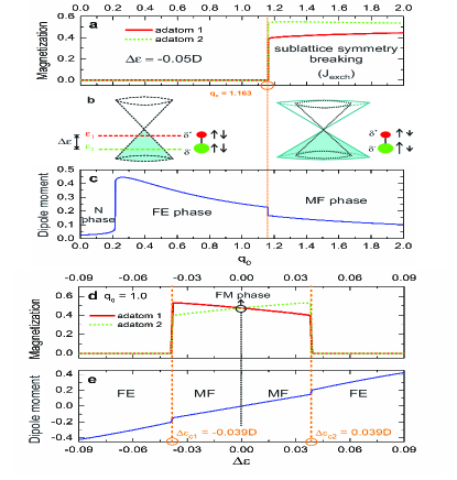
Figure 2: (Color online) (a) Magnetization of the system as a function of the Fano factor $q_{0}$ for fixed detuning $\Delta\varepsilon$. At critical value of the parameter $q_{c}$ the system is driven to the MF phase by a QPT. (b) The sketch illustrating the connection between the slope of the Dirac cones and magnetization of the system. (c) Dipole moment of the system as a function of the Fano factor $q_{0}$ for fixed detuning $\Delta\varepsilon$. After slow initial increase, the dipole moment experiences fast growing, followed by slow decrease and discontinuity at $q_{0}=q_{c}$. Rising of an anomalous MF phase for $q_{0}>q_{c}.$ (d) Magnetization of the system as a function of the detuning $\Delta\varepsilon$ for fixed Fano factor $q_{0}$. (e) Dipole moment of the system as a function of the detuning $\Delta\varepsilon$ for fixed $q_{0}$. The MF phase exists within the critical region $\Delta\varepsilon_{\text{{c}}1}<\Delta\varepsilon<\Delta\varepsilon_{\text{{c}2}},$ except for the FM phase where $\Delta\varepsilon=0.$ Otherwise, just the FE phase is present.

In Fig.2, we show the analysis of two spin-degenerate resonant states nearby and below the Dirac point. We consider the case for which the detuning between the energies of the two adatoms is non-zero, $\Delta\mathcal{E}=\mathcal{E}_{2}-\mathcal{E}_{1}=-0.05D,$ which leads to the appearance of the dipole moment $\delta^{-}-\delta^{+}=(<n_{2\uparrow}>+<n_{2\downarrow}>)-(<n_{1\uparrow}>+<n_{1\downarrow}>).$

For the Fano factor lying within the range $0.2<q_{0}<q_{c}=1.163$ (the critical point), the system is characterized only by the FE phase, since the MF behavior is absent as magnetizations $m_{l}=<n_{l\uparrow}>-<n_{l\downarrow}>$ of the adatoms are zero as can be seen at panels (a) and (b) of the same figure, where we verify that the local magnetic moments of the adatoms do not survive when embedded into graphene system. Fig.2(c) illustrates the dipole moment of the pair of adatoms. We should stress that $\delta^{-}-\delta^{+}$ and $m_{l}$ are local order parameters at the collinear sites of the adatoms, respectively for electric and magnetic degrees of freedom. Generally, the FE feature (electric polarization) of a system can be well-marked by evaluating the Berry phaseReview1 ; book , which depends upon the delocalized electronic Wannier functions spread over the crystal lattice. Here such an approach can not be invoked, since $\delta^{-}-\delta^{+}$ arises exclusively from the local FE feature of the adatoms, which are expected to exhibit wavefunctions extremely localized at their sites. As a result, this characteristic then prevents the use of the Berry phase method to recognize a phase as FE with long-range order parameter. In the range $q_{0}<0.2,$ $\delta^{-}-\delta^{+}$ is almost null as expected for the N phase, and then increases rapidly signifying the formation of the FE phase.

Physically, the FE feature, which here is not spontaneous, appears due to the charge imbalance between the magnetic adatoms, which is a purely electronic effect caused by the non-zero detuning $\Delta\mathcal{E}$ of their energy levels and the natural narrowing of the Dirac cones in the band structure outlined in Fig.2(b): the closer to the Dirac point is the adatom energy level $\mathcal{E}_{1}$ embedded in the graphene band structure, more emptied of electrons it should be (smaller red sphere with charge accumulation $\delta^{+}$ ). While the deeper is the embedded level $\mathcal{E}_{2}$ below the Dirac point, more electrons will accumulate in this adatom (bigger green sphere with charge accumulation $\delta^{-}$ ). Thus, as the graphene density of states decreases if one moves to the Dirac point (intrinsic bottleneck shape of the Dirac cones), the quantities $\delta^{+}$ and $\delta^{-},$ respectively for the levels $\mathcal{E}_{1}$ and $\mathcal{E}_{2}$ will be different as a result.

It is worth mentioning that in our approach, the formation of electric dipoles is thereby purely of electronic origin as we have discussed above. Lattice distortion is a direct consequence of the formation of such. A similar situation can be found in molecular compounds at the Mott metal-to-insulatorMariano1 ; Mariano2 ; Mariano3 and charge-ordering transitionsMariano4 ; Mariano5 . Although our approach does not cover lattice effects (ferroelasticity), given the presence of adatoms above and below the carbon atom (see Fig.1), one should expect that the sublattices move out-of-plane, but in opposite directions due to the charge imbalance $\delta^{+}$ and $\delta^{-}$ giving rise to a local lattice distortion. The evaluation of the electric dipole here concerns the sites of the adatoms and not a net contribution, being our analysis unaffected by the lattice distortion. To know the entire response, an ab-initio analysis should be implemented in order to find out if the polar catastrophe occurs compensating the electric dipole due to the adatoms. Here, we focus just on such a contribution.

Concerning the MF phase, our findings demonstrate that magnetic ordering $m_{l}$ is formed abruptly by means of a QPT when the Fano factor reaches its critical value $q_{0}=q_{c}$ as seen at Fig.2(a). At the same time, the value of the dipole moment $\delta^{-}-\delta^{+}$ experiences a jump down at $q_{0}=q_{c}$ (see Fig.2(c)). However, its value still remains non-zero and thus the system reaches the MF phase. We emphasize that both local order parameters $\delta^{-}-\delta^{+}$ and $m_{l}$ are finite and become coupled to each other (magnetoelectric effect) just for $q_{0}\geq q_{c},$ once for $q_{0}<q_{c}$ only $\delta^{-}-\delta^{+}\neq 0$ exists and local magnetic moments of adatoms are completely suppressed. This way, distinctly from standard multiferroicity, conjugate fields as electric and magnetic are not required for connecting these order parameters, being the Fano factor the unique control (tuning) parameter responsible for establishing the aforementioned correlation and the QPT as well. As a result, such features characterize the MF behavior here reported as anomalous. However, we do not discard that the conjugate fields (electric and magnetic) can change simultaneously the charge and magnetic order parameters, since such fields be applied to the system in the regime $q_{0}>q_{c},$ when the order parameters become correlated. For this situation, the multiferroicity here addressed would be ruled by the conjugate fields as usually occurs for bulk single-phase multiferroics.

As the Fano factor is inversely proportional to Fermi velocity (see Eq.(2)), the latter can be used as tuning parameter driving the QPT. Notice that in the MF phase, adatoms magnetize with the same sign revealing that they exhibit parallel magnetic moments, which means that emerging effective exchange coupling of their spins $J_{\text{{exch}}}=\text{{Re}}[\lambda_{l}^{\bar{\sigma}}\lambda_{\bar{l}}^{\bar{\sigma}}\Sigma^{2}(\mathcal{E}-\mathcal{E}_{\bar{l}}-\Sigma)^{-1}]$ (see Eq.(11)) is of Ruderman-Kittel-Kasuya-Yosida ferromagnetic-type, which manifests via graphene host as the self-energy $\Sigma$ ensures. Such a coupling arises from the increasing of the Fano factor value, which breaks strongly the adatom-graphene sublattice symmetry above the critical point, since the terms $\frac{t}{D}q_{0}\phi({\mathbb{k}})b_{\mathbb{k}\sigma}^{\dagger}d_{l\sigma}+\text{{H.c.}}$ become more pronounced with respect to $a_{\mathbb{k}\sigma}^{\dagger}d_{l\sigma}+\text{{H.c.}}$ in Eq.(1) for this regime. As aftermath, we find magnetic solutions and $J_{\text{{exch}}}$ is turned-on abruptly yielding the MF phase. This result matches the experimental findings reported in Ref.[STM, ], where a ferromagnetic coupling between magnetic adatoms is established by an exchange interaction via graphene, which is peculiar in a such a system: for the scenario of magnetic adatoms placed at carbon atoms belonging to the same sublattice, their local magnetic moments persist within the graphene environment and $J_{\text{{exch}}}$ is ferromagnetic-type, otherwise these moments become suppressed.

Here, the former situation occurs for $q_{0}\geq q_{c}$ and once in this range the Fano factor $q_{0}$ attains higher values, it forces the adatoms to perceive solely the sublattice B leading to $J_{\text{{exch}}}$ of ferromagnetic-type, while below the critical point $q_{0}<q_{c}$ the strength of $q_{0}$ is moderate, thus turning-off the magnetism at the adatoms, as aftermath of their couplings at the same footing with both sublattices. This situation should be distinguished with respect to the hollow setup considered by some of usLH , where a ferromagnetic exchange is not verified even considering magnetic adatoms. In such a case, the magnetic moments of the adatoms, within the Hubbard I approximation, become quenched as pointed out by our self-consistent calculations. For the bridge configuration, which is similar to the hollow case, we let it for the near future.

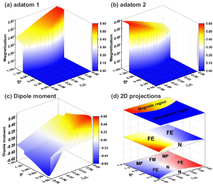
Figure 3: (Color online) (a)-(b) Magnetizations of the adatoms as a function of both $q_{0}$ and $\Delta\varepsilon$. (c) The dipole moment of an adatom pair as a function of both $q_{0}$ and $\Delta\varepsilon$ and finally (d), Upper plot: phase diagram for FM order parameter, middle plot: phase diagram for FE order parameter and lower plot: total phase diagram for N, FE, FM and MF phases.

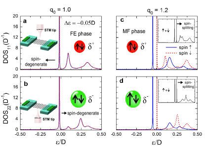
Figure 4: (Color online) (a)-(b) Spin-degenerate and charge split DOSs of the adatoms, due to the finite dipole moment, representing the FE phase, which can be probed by an STM tip. (c)-(d) In the MF phase, the DOSs are simultaneously charge and spin split.

If one uses the detuning $\Delta\mathcal{E}$ between the two collinear adatoms as driving parameter (which can be done e.g. by application of a bias parallel to the plane of the system) and keeps the Fano factor fixed, the system exhibits MF behavior in the finite range $\Delta\varepsilon_{\text{{c}}1}<\Delta\varepsilon<\Delta\varepsilon_{\text{{c}2}}$ as it can be seen at Figs.2(d,e). If the two adatoms are equal, naturally, there is no dipole moment in the system and their magnetizations are equal as observed in the point $\Delta\mathcal{E}=0,$ which is marked by the circle in the vertical dashed line in Fig.2(d) (FM phase). Notice that the dependence of $\delta^{-}-\delta^{+}$ on $\Delta\mathcal{E}$ shows linear trend as expected, with discontinuities at the critical points $\Delta\varepsilon_{\text{{c}}1}$ and $\Delta\varepsilon_{\text{{c}}2}.$

Fig.3 represents the 3D plots showing magnetization and dipole moment as a function of both $q_{0}$ and $\Delta\varepsilon$. The presence of the QPT characterized by abrupt jumps of the dipole moment and magnetization is clearly visible at these plots. The full phase diagram of the system, which is the main result of the current work is shown at Fig.3(d).

As demonstrated in Ref.[Shelykh, ] by one of us, one way to tune the slope of the Dirac cones is to couple electronic states in free-standing graphene to linear polarized dressing light field. To detect the FE phase, one can employ STM tip measurements of differential conductance for suspended grapheneDresselhaus (insets of Figs.4(a,b)) which can probe $\text{DOS}_{ll}^{\uparrow}+\text{DOS}_{ll}^{\downarrow}.$ The FE feature is then revealed, as ensured by Eq.(9), just by determining the areas under the curves of $\text{DOS}_{22}^{\uparrow}+\text{DOS}_{22}^{\downarrow}$ and $\text{DOS}_{11}^{\uparrow}+\text{DOS}_{11}^{\downarrow},$ which give respectively distinct charge accumulations $\delta^{-}=<n_{2\uparrow}>+<n_{2\downarrow}>$ and $\delta^{+}=<n_{1\uparrow}>+<n_{1\downarrow}>$ that characterize the local ordering parameter $\delta^{-}-\delta^{+}\neq 0$, since we can notice from panels (a,b) different areas. We should pay particular attention that in the FE phase, a single pronounced spin-degenerate peak nearby the Dirac point is also a hallmark of such a phase.

A sudden spin-splitting (panels (c,d) and insets with $q_{0}=1.2$), due to the QPT, of the already charge split resonant states (panels (a,b) with $q_{0}=1$) is verified in the MF phase. Such a splitting can be detectable just by employing an unpolarized STM tip, which reveals in $\text{DOS}_{ll}^{\uparrow}+\text{DOS}_{ll}^{\downarrow},$ a pair of peaks close to the Dirac point emerging instead of the only single verified in FE phase, here appearing depicted in the insets of panels (c,d) of the same figure and being very similar to the result observed experimentally in Ref.[STM, ], due to local magnetic moments of adatoms. It means that besides the feature of $\delta^{-}-\delta^{+}\neq 0$ as aftermath of distinct areas under the curves of $\text{DOS}_{22}^{\uparrow}+\text{DOS}_{22}^{\downarrow}$ and $\text{DOS}_{11}^{\uparrow}+\text{DOS}_{11}^{\downarrow}$ (panels (c,d)), the pair of peaks in the neighborhood of the Dirac point (insets of these panels) constitutes the capital fingerprint for confirming the MF phase. Thus the presence of the FE ordering is revealed by the charge split peaks in the DOSs as shown at Figs.4(a,b), while the transition into the MF phase is accompanied by the emergence of the additional spin splitting of the peaks as shown at Figs.4(c,d). Thereby, we consider these features as the smoking-gun of the QPT transition from the FE phase to MF, which experimentalists can pursuit for.

IV Conclusions

In summary, we have shown that graphene with collinear pair of magnetic adatoms can be driven into a MF phase via a QPT by changing the slope of the Dirac cones. To detect such a QPT, we claim that the proper tool to this aim is the STM experiment reported in Ref.[STM, ].

V Acknowledgments

This work was supported by CNPq, CAPES, 2015/23539-8 São Paulo Research Foundation (FAPESP) and FP7 IRSES project QOCaN. I.A.S acknowledges the support from Rannis project BOFEHYSS, Horizon2020 RISE project CoExAn and 5-100 program of Russian Federal Government.

References

- (1) Daniel Khomskii, Physics 2, 20 (2009).
- (2) W. Eerenstein, N. D. Mathur, and J. F. Scott, Nature 442, 759 (2006).
- (3) Y. Tokura, S. Seki, and N. Nagaosa, Rep. Prog. Phys. 77, 076501 (2014).
- (4) R. Ramesh and N. A. Spaldin, Nature Mater. 6, 21 (2007).
- (5) T. Kimura, T. Goto, H. Shintani, K. Ishizaka, T. Arima, and Y. Tokura, Nature 426, 55 (2003).
- (6) N. Hur, S. Park, P. A. Sharma, J. S. Ahn, S. Guha, and S-W. Cheong, Nature 429, 392 (2004).
- (7) S.-W. Cheong and M. Mostovoy, Nature Mater. 6, 13 (2007).
- (8) M. Fiebig, J. Phys. D, 38, R123 (2005).
- (9) L. Seixas, A. S. Rodin, A. Carvalho, and A. H. Castro Neto, Phys. Rev. Lett. 116, 206803 (2016).
- (10) M. Pregelj, A. Zorko, O. Zaharko, Z. Kutnjak, M. Jagodic, Z. Jaglicic, H. Berger, M. de Souza, C. Balz, M. Lang, and D. Arcon, Phys. Rev. B 82, 144438 (2010).
- (11) G. Giovannetti, R. Nourafkan, G. Kotliar, and M. Capone, Phys. Rev. B 91, 125130 (2015).
- (12) P. Lunkenheimer, J. Müller, S. Krohns, F. Schrettle, A. Loidl, B. Hartmann, R. Rommel, M. de Souza, C. Hotta, J. A. Schlueter, and M. Lang, Nature Mater. 11, 755 (2012).
- (13) V. Meunier, A. G. Souza Filho, E. B. Barros, and M. S. Dresselhaus, Rev. Mod. Phys. 88, 025055 (2016).
- (14) A. H. Castro Neto, F. Guinea, N. M. R. Peres, K. S. Novoselov, and A. K. Geim, Rev. Mod. Phys. 81, 109 (2009).
- (15) B. Uchoa, L. Yang, S.-W.Tsai, N. M. R. Peres, and A. H. Castro Neto, New J. Phys. 16, 013045 (2014).
- (16) P. W. Anderson, Phys. Rev. 124, 41 (1961).
- (17) A. C. Seridonio, M. Yoshida, and L. N. Oliveira, Europhys. Lett. 86, 67006 (2009).
- (18) Z.-G. Zhu, K.-H. Ding, and J. Berakdar, Europhys. Lett. 90, 67001 (2010).
- (19) H. G.-Herrero, J. M. G.-Rodríguez, P. Mallet, M. Moaied, J. J. Palacios, C. Salgado, M. M. Ugeda, J.-Y. Veuillen, F. Yndurain, and I. Brihuega, Science 352, 437 (2016).
- (20) J. Hubbard, Proc. R. Soc. Lond. A, 281, 401 (1964).
- (21) P. Gegenwart, Q. Si, and F. Steglich, Nature Physics 4, 186 (2008).
- (22) R. Resta and D. Vanderbilt, Topics in Applied Physics, 105, 31, (2007).
- (23) S. R. Hassan, A. Georges, and H. R. Krishnamurthy, Phys. Rev. Lett. 94, 036402 (2005).
- (24) M. de Souza, A. Brühl, Ch. Strack, B. Wolf, D. Schweitzer, and M. Lang, Phys. Rev. Lett. 99, 037003 (2007).
- (25) M. de Souza and L. Bartosch, J. Phys. Cond.: Matter, 27, 053203 (2015).
- (26) M. de Souza, P.F.-Leylekian, A. Moradpour, J.-P. Pouget, and M. Lang, Phys. Rev. Lett. 101, 216403 (2008).
- (27) M. de Souza and J.-P. Pouget, J. Phys. Cond.: Matter, 25, 343201 (2013).
- (28) L.H. Guessi, R. S. Machado, Y. Marques, L. S. Ricco, K. Kristinsson, M. Yoshida, I. A. Shelykh, M. de Souza, and A. C. Seridonio, Phys. Rev. B 92, 045409 (2015).
- (29) K. Kristinsson, O. V. Kibis, S. Morina, and I. A. Shelykh, Sci. Rep. 6, 20082 (2016).