Error analysis of a variational multiscale stabilization for convection-dominated diffusion equations in 2d

Abstract

We formulate a stabilized quasi-optimal Petrov-Galerkin method for singularly perturbed convection-diffusion problems based on the variational multiscale method. The stabilization is of Petrov-Galerkin type with a standard finite element trial space and a problem-dependent test space based on pre-computed fine-scale correctors. The exponential decay of these correctors and their localisation to local patch problems, which depend on the direction of the velocity field and the singular perturbation parameter, is rigorously justified. Under moderate assumptions, this stabilization guarantees stability and quasi-optimal rate of convergence for arbitrary mesh Péclet numbers on fairly coarse meshes at the cost of additional inter-element communication.

1 Introduction

Given a domain $\Omega\subset\mathbb{R}^{2}$, a singular perturbation parameter $0<\epsilon\leq 1$, a velocity field $b\in(L^{\infty}(\Omega))^{2}$ and some force $f\in H^{-1}(\Omega)$, the convection-diffusion equation seeks $u\in V:=H^{1}_{0}(\Omega)$ such that

$$-\epsilon\Delta u+b\cdot\nabla u =f\quad\text{in }\Omega,$$ (1.1)

$$u =0\quad\text{on }\partial\Omega.$$

We assume that the velocity field $b$ is incompressible, i.e., $\nabla\cdot b=0$. The focus of this paper is on the convection-dominated regime with large Péclet number $\mathrm{Pe}=\left\|b\right\|_{L^{\infty}\left(\Omega\right)}/\epsilon$.

For reasonable small Péclet numbers, classical Galerkin finite element methods (FEMs) perform well. However, if the Péclet number increases, then steep gradients of $u$ occur and boundary layers appear, which require a much finer mesh to capture the characteristic width of those boundary layers. Consequently, local corrections are needed at those layers and a numerical method in which the smooth solution regions are not polluted by those layers is desirable. The thickness of the parabolic layer is $\mathcal{O}(\sqrt{\epsilon})$ and $\mathcal{O}(\epsilon)$ for the exponential layer, which have to be resolved for a stable approximation with a standard Galerkin FEM. Furthermore, it holds that $\left|u\right|_{H^{1}\left(\Omega^{*}\right)}=\mathcal{O}(\epsilon^{-\frac{1}{4}})$ and $\left|u\right|_{H^{1}\left(\Omega^{o}\right)}=\mathcal{O}(\epsilon^{-\frac{1}{2}})$ with small neighbourhoods $\Omega^{*}$ and $\Omega^{o}$ of the parabolic and the exponential boundary layer, respectively [23, 14].

Numerous numerical methods have been proposed in the past few decades aiming at solving the convection dominated problem (1.1) efficiently and accurately. Upwinding methods for stabilization of the exponential boundary layers combined with refinement near the parabolic boundary layers are formulated. Among them are streamline upwind/Petrov-Galerkin method (SUPG) or Galerkin least squares method (GLS) [10, 6], hp finite element methods [17, 18], discontinuous Petrov-Galerkin methods (DPG) [8], residual-free bubble approaches (RFB) [2, 5, 4], methods with an additional non-linear diffusion [1], methods with stabilization by local orthogonal sub-scales [7] and hybridizable discontinuous Galerkin (HDG) methods [22]. Among the multiscale methods are variational multiscale methods (VMS) [13, 15], multiscale finite element methods (MsFEM) [19, 3], multiscale hybrid-mixed methods (MHM) [12] and local orthogonal decomposition methods (LOD) [9]. Specifically, the residual-based stabilization methods (SUPG, GLS and RFB) incorporate global stability properties into high accuracy in local regions away from boundary layers. We refer to [23] for an overview of robust numerical methods for singular perturbed problems. In this paper, our focus is on the construction and the error analysis of a stable and accurate LOD method based on [13, 21, 16].

VMS was designed for solving multiscale problems by embedding fine-scale information into the coarse-scale framework. Essentially, the efficiency and accuracy rely on the construction of a problem-dependent stable projector from a larger fine space onto a relatively much smaller coarse space. Our motivation for this paper is originated from [13], where the authors derived an explicit formula for the one-dimensional fine-scale Green’s function arising in VMS. The smaller the support of the fine-scale Green’s function, the more favorable the localized method (e.g., [16, 21]) in solving (1.1). In particular, the authors compared the fine-scale Green’s functions derived by the $L^{2}$-projector with that derived by the $H_{0}^{1}$-projector, and concluded that the latter outweighed the former in the one-dimensional case. In addition, examples were shown for the two-dimensional case that the $H_{0}^{1}$-projector would exceed the $L^{2}$-projector as well. There is a recent work [9] on the convection-diffusion problem employing the $L^{2}$-projector in the framework of VMS and LOD. The author shows convergence of the localized method and tests the method using $H_{0}^{1}$-projector and claim that the superiority of $H_{0}^{1}$-projector over the $L^{2}$-projector is not valid for the two-dimensional case.

In the one-dimensional case, the $H^{1}_{0}$ projection equals the nodal interpolation. Therefore, another possible generalization of the 1d case to higher dimensions is to use nodal interpolation in the VMS. This approach was previously utilised in [15] and seems to work better than averaging type operators. In this paper, we show that a VMS based on the nodal interpolation operator coupled with a Petrov-Galerkin method is stable and locally quasi-optimal for the convection-dominated problem (1.1) with no spurious oscillations and no smearing. As for other elliptic PDEs the ideal VMS is turned into a practical method by localizing the support of the VMS basis functions [20]. Inspired by the numerical results of the fine-scale Green’s functions displayed in [13] and the proof in our paper as well, a $b$-biased local region is proposed as the numerical domain for approximating the ideal method. The convergence of this localization is proved under the assumption that the local region is sufficiently large.

The remainder of this paper is organized as follows. In Section 2, a detailed description of the problem considered in this paper is shown. In Section 3, we propose a new VMS method based on the nodal interpolation and denote it as the ideal method. Its stability and local quasi-optimality are displayed. In Section 4, we estimate the error of the global correctors outside a certain local patch and show an exponential decay of the error with respect to the size of the local patch. Inspired by the results in Section 4, we formulate the localization algorithm in Section 5 for the ideal method proposed in Section 3, and display the stability of this algorithm as well as the convergence. A numerical experiment is provided in Section 6 for the validation of our method and we end this paper with conclusions in Section 7.

2 Model problem and standard finite elements

We assume that the parameter $\epsilon\leq 1$ and $b\in L^{\infty}(\Omega;\mathbb{R}^{2})$ is a divergence-free vector field and we define the bilinear form $a$ on $V\times V$ associated to (1.1) by

$$a(u,v)=\epsilon\int_{\Omega}\nabla u\cdot\nabla v\,dx+\int_{\Omega}(b\cdot\nabla u)\,v\,dx\qquad\text{for all }u,v\in V.$$ (2.1)

Since $\nabla\cdot b=0$, an integration by parts implies that the bilinear form $a$ is $V$-elliptic, i.e.,

$$a(v,v) =\epsilon\left|v\right|_{H^{1}\left(\Omega\right)}^{2}\qquad\text{ for all }v\in V.$$ (2.2)

Furthermore, a Poincaré-Friedrichs inequality leads to the existence of some $C(\Omega,b)$ that may depend on (the diameter of) the domain $\Omega$ and the $L^{\infty}$-norm of $b$ such that $a$ is continuous, i.e., for all $u,v\in V$ it holds that

$$a(u,v) \leq\epsilon\left|u\right|_{H^{1}\left(\Omega\right)}\left|v\right|_{H^{1}\left(\Omega\right)}+\|b\|_{L^{\infty}(\Omega)}\left|u\right|_{H^{1}\left(\Omega\right)}\left\|v\right\|_{L^{2}\left(\Omega\right)}$$ (2.3)

$$\leq C(\Omega,b)\left|u\right|_{H^{1}\left(\Omega\right)}\left|v\right|_{H^{1}\left(\Omega\right)}.$$

Here, we used that $\epsilon\leq 1$. Throughout this paper, $A\lesssim B$ abbreviate that there exists a constant $C>0$ independent of $\epsilon$, $h$ and $H$ ($h$ and $H$ will be defined later), such that $A\leq CB$, and let $A\gtrsim B$ be defined as $B\lesssim A$ and $A\approx B$ abbreviates $A\lesssim B\lesssim A$. We assume that $\left\|b\right\|_{L^{\infty}\left(\Omega\right)}\approx 1$. Let $\langle\bullet,\bullet\rangle_{H^{-1}(\Omega)\times H^{1}_{0}(\Omega)}$ denote the dual pairing of $H^{-1}(\Omega)$ and $H^{1}_{0}(\Omega)$.

We consider the variational form of (1.1):

$$\left\{\begin{aligned} &\text{find $u\in V$ such that for all }v\in V\\ &a(u,v)=\langle f,v\rangle_{H^{-1}(\Omega)\times H^{1}_{0}(\Omega)}.\end{aligned}\right.$$ (2.4)

By virtue of the $V$-ellipticity and $V$-continuity of $a$ from (2.2) and (2.3) and the Lax-Milgram lemma, problem (2.4) has a unique solution in $V$.

Let $\mathcal{T}_{h}$ be a shape-regular triangulation of the domain $\Omega$, where $h$ represents the minimal diameter of all triangles in $\mathcal{T}_{h}$. Given a triangulation $\mathcal{T}$, let

$${\mathcal{P}}_{1}(\mathcal{T}) :=\{{v}\in C^{0}(\Omega)\mid{v}|_{K}\in P^{1}(K)\mbox{ for all }K\in\mathcal{T}\},$$

denote the space of piecewise linear finite elements and define $V_{h}:={\mathcal{P}}_{1}(\mathcal{T}_{h})\cap V$.

Let $u_{h}\in V_{h}$ denote the reference solution, which is defined as the Galerkin approximation that satisfies

$$a(u_{h},v_{h})=\langle f,v_{h}\rangle_{H^{-1}(\Omega)\times H^{1}_{0}(\Omega)}\qquad\text{for all }v_{h}\in V_{h}.$$ (2.5)

Taking advantage of the ellipticity and continuity of $a$ from (2.2) and (2.3) on $V\times V\supset V_{h}\times V_{h}$, the Lax-Milgram lemma implies that the fine-scale solution $u_{h}$ of (2.5) exists and is unique on $V_{h}$.

We assume that $\epsilon\ll 1$ is a small parameter and that $\mathcal{T}_{h}$ resolves $\epsilon$ in the sense that $u_{h}$ is a good approximation of $u$, e.g., if

$$h_{\mathrm{max}}\|b\|_{L^{\infty}(\Omega)}/\epsilon\lesssim 1$$ (2.6)

with the maximal mesh-size $h_{\mathrm{max}}$ of $\mathcal{T}_{h}$. It holds that

$$\left|u-u_{h}\right|_{H^{1}\left(\Omega\right)}\lesssim\left(1+\frac{h_{\mathrm{max}}\|b\|_{L^{\infty}(\Omega)}}{\epsilon}\right)\inf_{v_{h}\in V_{h}}\left|u-v_{h}\right|_{H^{1}\left(\Omega\right)}.$$

If, in addition, the solution $u$ of (2.4) satisfies $u\in H^{2}(\Omega)$, standard interpolation estimates lead to

$$\left|u-u_{h}\right|_{H^{1}\left(\Omega\right)}\lesssim h_{\mathrm{max}}\left(1+\frac{h_{\mathrm{max}}\|b\|_{L^{\infty}(\Omega)}}{\epsilon}\right)\|u\|_{H^{2}(\Omega)},$$

with a hidden constant independent of $\epsilon$. Note, however, that $\|u\|_{H^{2}(\Omega)}$ depends on $\epsilon$.

3 The ideal method

In this section we introduce a variational multiscale method based on the nodal interpolation, which yields a locally best-approximation of the reference solution $u_{h}\in V_{h}$ from (2.5) and which is computed on a feasible coarse underlying mesh $\mathcal{T}_{H}$. We assume that $\mathcal{T}_{H}$ is a regular quasi-uniform triangulation of the domain $\Omega$ with maximal mesh-size $H$, such that $\mathcal{T}_{h}$ is a refinement of $\mathcal{T}_{H}$. Let $\mathcal{N}_{H}$ denote the nodes in $\mathcal{T}_{H}$ and $\mathrm{mid}_{K}$ the baricenter for each coarse element $K\in\mathcal{T}_{H}$. The maximal mesh-size $H$ of $\mathcal{T}_{H}$ represents a computationally feasible scale that is typically much larger than $\epsilon$. Altogether, the target regime is then

$$0<h<\epsilon\ll H\lesssim 1.$$

Define $V_{H}={\mathcal{P}}_{1}(\mathcal{T}_{H})\cap V$ and let $I_{H}:V_{h}\rightarrow V_{H}$ denote the nodal interpolation. Note that $I_{H}$ acts only on finite element functions and is, hence, well defined. It holds,

$$H^{-1}\left\|v-I_{H}v\right\|_{L^{2}\left(T\right)}+\left|I_{H}v\right|_{H^{1}\left(T\right)}\leq C_{I_{H}}\big{(}\tfrac{H}{h}\big{)}\left|v\right|_{H^{1}\left(T\right)}.$$ (3.1)

Indeed, we have [24]

$$C_{I_{H}}\big{(}\tfrac{H}{h}\big{)}\lesssim\begin{cases}1&\quad\text{ in one dimension},\\ \log{\frac{H}{h}}&\quad\text{ in two dimensions},\\ \frac{H}{h}&\quad\text{ in three dimensions}.\end{cases}$$

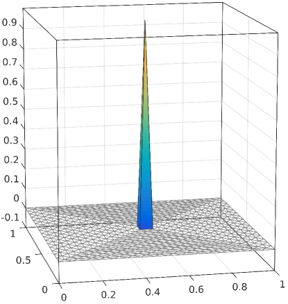
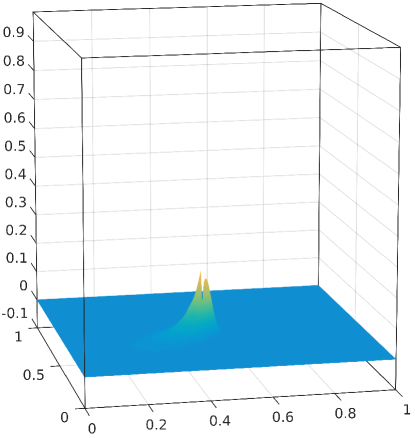
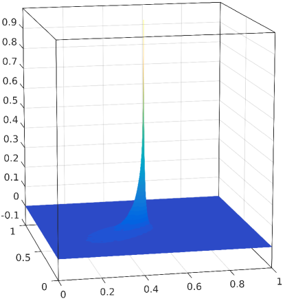
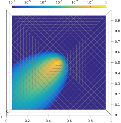
Figure 1: Standard nodal basis function $\lambda_{z}$ with respect to the coarse mesh $\mathcal{T}_{H}$ (top left), corresponding ideal corrector $\mathcal{C}\lambda_{z}$ (top right), and corresponding test basis function $(1-\mathcal{C})\lambda_{z}$ (bottom left). The bottom right figure shows a top view on the modulus of test basis function $(1-\mathcal{C})\lambda_{z}$ with logarithmic color scale to illustrate the exponential decay property. The underlying data is $b=[\cos(0.7),\sin(0.7)]$ and $\epsilon=2^{-7}$.

Given $v_{H}\in V_{H}$, define the subscale corrector $\mathcal{C}:V_{H}\to\mathrm{Ker}I_{H}$ by

$$a(w,\mathcal{C}v_{H})=a(w,v_{H})\qquad\text{for all }w\in\mathrm{Ker}I_{H}.$$ (3.2)

The well-posedness of (3.2) follows from the ellipticity and continuity of $a$, since $\mathrm{Ker}I_{H}\subset V$.

Now we are ready to define the multiscale test space as

$$W_{H}:=(1-\mathcal{C})V_{H}.$$

Note that (3.2) implies that

$$W_{H}=\{w\in V_{h}:\forall v\in\mathrm{Ker}I_{H},a(v,w)=0\}.$$

The Petrov-Galerkin method for the approximation of (2.5) based on the trial-test pairing $(V_{H},W_{H})$ defined above seeks $u_{H}\in V_{H}$ satisfying

$$a(u_{H},w_{H})=\langle f,w_{H}\rangle_{H^{-1}(\Omega)\times H^{1}_{0}(\Omega)}\qquad\text{for all }w_{H}\in W_{H}.$$ (3.3)

Note that (3.3) is a variational characterization of $I_{H}$ in the sense that, for all $w_{H}\in W_{H}$, we have

$$a(I_{H}u_{h},w_{H})=a(I_{H}u_{h}-u_{h},w_{H})+a(u_{h},w_{H})=(f,w_{H}),$$

where the last equality follows from (3.2), (2.5) and the fact that $I_{H}u_{h}-u_{h}\in\mathrm{Ker}I_{H}$. Since $\mathrm{dim}V_{H}=\mathrm{dim}W_{H}$, it follows that $u_{H}=I_{H}u_{h}\in V_{H}$ is the unique solution of (3.3) and the ideal method inherits favourable stability and approximation properties from the interpolation $I_{H}$. To be more precise, we have the following proposition, which follows directly from the identity $u_{H}=I_{H}u_{h}$ and (3.1).

Proposition 3.1 (Stability and local quasi-optimality of the ideal method).

For any $f\in H^{-1}(\Omega)$, the ideal Petrov-Galerkin method (3.3) admits a unique solution $u_{H}$ in the standard finite element space $V_{H}$. The method is stable in the sense that

$$\left|u_{H}\right|_{H^{1}\left(\Omega\right)}\leq C_{I_{H}}\big{(}\tfrac{H}{h}\big{)}\left|u_{h}\right|_{H^{1}\left(\Omega\right)},$$

where $u_{h}\in V_{h}$ denotes the reference solution that solves (2.5). Note that the constant $C_{I_{H}}\big{(}\tfrac{H}{h}\big{)}$ is independent of $\epsilon$, but may depend on $H/h$.

Moreover, for any $T\in\mathcal{T}_{H}$, we have the local best-approximation result

$$\left|u_{h}-u_{H}\right|_{H^{1}\left(T\right)}\leq C_{I_{H}}\big{(}\tfrac{H}{h}\big{)}\min\limits_{v_{H}\in V_{H}}\left|u_{h}-v_{H}\right|_{H^{1}\left(T\right)}.$$

Remark 3.2.

The stability and quasi-optimality of Proposition 3.1 also holds for any other norm in which $I_{H}$ is stable.

We admit that the corrector problems (3.2) are global problems on the fine triangulation $\mathcal{T}_{h}$ which have to be precomputed for the solving of (3.3). This would result in a number of $\mathrm{dim}(V_{H})$ problems of dimension $O(\mathrm{dim}(V_{h}))$ which is comparable of solving the original problem (1.1) on a fine grid by an efficient standard method. This makes the VMS (3.3) not realistic. However, it can be observed in Figure 1 that the corrector of functions with local support are still quasi-local in the sense that they decay exponentially. This allows for an approximation of the corrector by functions of local support. In the next section, the exponential decay will be made rigorous, while Section 5 proves stability and approximation properties for a localization strategy.

We end this section with a proof of the stability in the classical inf-sup sense, although the method is perfectly stable in the sense of Proposition 3.1. This result will be used in Section 5 to prove well posedness of the localized version of (3.3).

Lemma 3.3 (Stability).

The trial-test pairing $(V_{H},W_{H})$ satisfies the inf-sup condition

$$\inf\limits_{w_{H}\in W_{H}\setminus\{0\}}\sup\limits_{u_{H}\in V_{H}\setminus\{0\}}\frac{a(u_{H},w_{H})}{\left|u_{H}\right|_{H^{1}\left(\Omega\right)}\left|w_{H}\right|_{H^{1}\left(\Omega\right)}}\geq\frac{\epsilon}{C_{I_{H}}\big{(}\tfrac{H}{h}\big{)}}.$$ (3.4)

Proof.

Given $w_{H}\in W_{H}$, take $u_{H}=I_{H}(w_{H})\in V_{H}$. Then by (3.1),

$$\left|u_{H}\right|_{H^{1}\left(\Omega\right)}\leq C_{I_{H}}\big{(}\tfrac{H}{h}\big{)}\left|w_{H}\right|_{H^{1}\left(\Omega\right)}.$$ (3.5)

Note that $I_{H}(w_{H})-w_{H}\in\mathrm{Ker}I_{H}$. By (3.2), we have

$$a(u_{H},w_{H})=a(I_{H}(w_{H}),w_{H})=a(w_{H},w_{H})=\epsilon\left|w_{H}\right|_{H^{1}\left(\Omega\right)}^{2},$$ (3.6)

where the last inequality follows from $\nabla\cdot b=0$.

We obtain the result by the application of (3.5). ∎

4 Exponential decay of element correctors

This section is devoted to the proof of the exponential decay of element correctors defined in the following. Given $\omega\subset\Omega$, define the local bilinear form

$$a_{\omega}(u,v):=\epsilon\int_{\omega}\nabla u\cdot\nabla v\,dx+\int_{\omega}(b\cdot\nabla u)\,v\,dx\qquad\text{for all }u,v\in V$$ (4.1)

and let the local corrector $\mathcal{C}_{T}:V_{H}\to\mathrm{Ker}I_{H}$ be defined for any $v_{H}\in V_{H}$ by

$$a(w,\mathcal{C}_{T}v_{H})=a_{T}(w,v_{H})\qquad\text{for all }w\in\mathrm{Ker}I_{H}.$$ (4.2)

Note that $\mathcal{C}=\sum_{T\in\mathcal{T}_{H}}\mathcal{C}_{T}$ holds for the corrector $\mathcal{C}$ defined by (3.2).

We consider the case that $\epsilon\leq H$. In the following we restrict ourselves to a constant vector field $b$ and w.l.o.g. $|b|=1$; see Remark 4.4 below for a discussion for non-constant vector fields $b$. Define $t$ as a unit vector in $\mathbb{R}^{2}$, s.t. $t\cdot b=0$. Define a rectangle $S_{T,\ell,b}$ for each $T\in\mathcal{T}_{H}$ and $\ell\in\mathbb{N}_{+}$ by

$$S_{T,\ell,b} :=\Omega\cap\operatorname{conv}\{\mathrm{mid}_{T}-\ell Ht+\ell Hb,\mathrm{mid}_{T}+\ell Ht+\ell Hb,$$ (4.3)

$$\qquad\qquad\qquad\qquad\mathrm{mid}_{T}-\ell Ht-\ell H^{2}b/\epsilon,\mathrm{mid}_{T}+\ell Ht-\ell H^{2}b/\epsilon\}.$$

We do not assume that $b$ is aligned with the triangulation and therefore we define the patches $\Omega_{T,\ell,b}$ by

$$\Omega_{T,\ell,b}:=\cup\{T^{\prime}\in\mathcal{T}_{H}\mid T^{\prime}\cap S_{T,\ell,b}\neq\emptyset\}\supset S_{T,\ell,b}.$$

See Figure 2 for an illustration. For fixed $\ell\in\mathbb{N}_{+}$, the element patches have finite overlap in the sense that there exists a constant $C_{\mathrm{ol},\ell}(\epsilon)>0$, s.t.,

$$\max_{K\in\mathcal{T}_{H}}\#\{T\in\mathcal{T}_{H}\mid K\subset\Omega_{T,\ell,b}\}\leq C_{\mathrm{ol},\ell}(\epsilon).$$ (4.4)

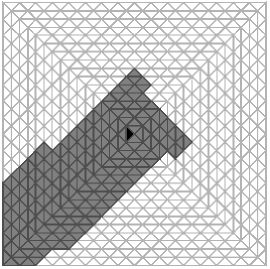
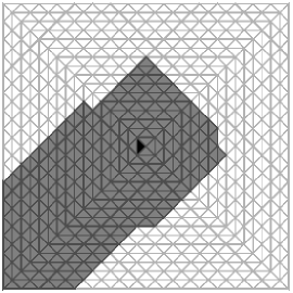
Figure 2: Element patches $\Omega_{T,\ell,b}$ for $b=[\cos(0.7),\sin(0.7)]$, $\epsilon=2^{-7}$ and $\ell=1,2,3$ (from left to right) as they are used in the localised corrector problem (5.1).

Theorem 4.1.

Let $T\in\mathcal{T}_{H}$ and $v_{H}\in V_{H}$ and let $\mathcal{C}_{T}v_{H}$ denote the corresponding local subscale corrector as defined in (4.2). Then we have

$$\left|\mathcal{C}_{T}v_{H}\right|_{H^{1}\left(\Omega\setminus S_{T,\ell,b}\right)}\lesssim\beta^{\ell}\left|\mathcal{C}_{T}v_{H}\right|_{H^{1}\left(\Omega\right)}.$$ (4.5)

The constant $\beta$ reads

$$\beta=\left(\frac{4C_{I_{H}}\big{(}\tfrac{H}{h}\big{)}+3C_{I_{H}}\big{(}\tfrac{H}{h}\big{)}^{2}}{1+4C_{I_{H}}\big{(}\tfrac{H}{h}\big{)}+3C_{I_{H}}\big{(}\tfrac{H}{h}\big{)}^{2}}\right)^{1/2}<1$$ (4.6)

and is bounded away from 1.

Before going to the proof of this theorem, we express the exponential decay in terms of patches in the following corollary. This is a direct consequence of Theorem 4.1 and the definition of $\Omega_{T,\ell,b}$.

Corollary 4.2.

Let $T\in\mathcal{T}_{H}$ and $v_{H}\in V_{H}$ and let $\mathcal{C}_{T}v_{H}$ denote the corresponding local subscale corrector as defined in (4.2). Then we have

$$\left|\mathcal{C}_{T}v_{H}\right|_{H^{1}\left(\Omega\setminus\Omega_{T,\ell,b}\right)}\leq\left|\mathcal{C}_{T}v_{H}\right|_{H^{1}\left(\Omega\setminus S_{T,\ell,b}\right)}\lesssim\beta^{\ell}\left|\mathcal{C}_{T}v_{H}\right|_{H^{1}\left(\Omega\right)}$$ (4.7)

with $\beta<1$ from (4.6).

Remark 4.3.

Recall that in this two-dimensional situation $C_{I_{H}}\big{(}\tfrac{H}{h}\big{)}\lesssim\log(\tfrac{H}{h})$ for $C_{I_{H}}\big{(}\tfrac{H}{h}\big{)}$ from (3.1). Then given fixed $H\in(0,1)$ and let $h\to 0$, the constant $\beta$ scales as

$$1-\beta^{2}\gtrsim\frac{1}{1+\log(h)^{2}}.$$

In the three dimensional case, Theorem 4.1 could essentially be proven in the same way, but the dependence of $C_{I_{H}}\big{(}\tfrac{H}{h}\big{)}$ on $H/h$ is algebraic so that the decay rate deteriorates very fast.

Proof of Theorem 4.1.

The crucial point in the proof is (4.10) below, which exploits the direction of $b$. This allows for patches that are only enlarged in the direction of $-b$. The remaining part of the proof then essentially follows as in [16].

Define a cut-off function

$$\eta:=1-\eta_{1}\eta_{2},$$

where $0\leq\eta_{1}(x)\leq 1$ and $0\leq\eta_{2}(x)\leq 1$ are one-dimensional continuous piecewise affine cut-off functions along $t$ and $b$, respectively. Recall that $\mathrm{mid}_{T}$ denotes the baricenter of a coarse element $T$, $|b|=1$ and $t$ is a unit vector orthogonal to $b$. We define $\eta_{1}$ and $\eta_{2}$ by

$$\eta_{1}(x)=\left\{\begin{aligned} 1&\quad\text{ if }|(x-\mathrm{mid}_{T})\cdot t|\leq(\ell-1)H;\\ 0&\quad\text{ if }|(x-\mathrm{mid}_{T})\cdot t|\geq\ell H\end{aligned}\right.$$ (4.8)

and

$$\eta_{2}(x)=\left\{\begin{aligned} 1&\quad\text{ if }-(\ell-1)H\leq-(x-\mathrm{mid}_{T})\cdot b\leq(\ell-1)\frac{H^{2}}{\epsilon};\\ 0&\quad\text{ if }-(x-\mathrm{mid}_{T})\cdot b\geq\ell\frac{H^{2}}{\epsilon}\;\text{ or }\;-(x-\mathrm{mid}_{T})\cdot b\leq-\ell H.\end{aligned}\right.$$ (4.9)

We obtain from the construction above that $\nabla\eta_{1}(x)\cdot b=0$ for all $x\in\Omega$ and $\eta_{1}\leq 1$. Moreover, since $-(b\cdot\nabla\eta_{2}(x))\leq 0$ if $0\leq(x-\mathrm{mid}_{T})\cdot b$, we deduce

$$-b\cdot\nabla\eta=-(b\cdot\nabla\eta_{1})\eta_{2}-(b\cdot\nabla\eta_{2})\eta_{1}=-(b\cdot\nabla\eta_{2})\eta_{1}\leq\frac{\epsilon}{H^{2}}.$$ (4.10)

Furthermore, $\eta|_{S_{T,\ell-1,b}}=0$ and $\eta|_{\Omega\setminus S_{T,\ell,b}}=1$, and $\eta$ is bounded between 0 and 1 and satisfies the Lipschitz continuity

$$\left\|\nabla\eta\right\|_{L^{\infty}\left(\Omega\right)}\leq 2/H.$$ (4.11)

Note that $\mathrm{supp}(\nabla\eta)\subset S_{T,\ell,b}\setminus S_{T,\ell-1,b}$.

Let $(\bullet,\bullet):=(\bullet,\bullet)_{L^{2}(\Omega)}$ denote the $L^{2}$ scalar product and define $\varphi:=\mathcal{C}_{T}v_{H}$. Due to $\nabla\cdot b=0$, we have $(b\cdot\nabla(\eta\varphi),\eta\varphi)=0$, and

$$\epsilon\left|\varphi\right|_{H^{1}\left(\Omega\setminus S_{T,\ell,b}\right)}^{2} \leq\epsilon(\nabla(\eta\varphi),\nabla(\eta\varphi))+(b\cdot\nabla(\eta\varphi),\eta\varphi)$$

$$=\epsilon(\nabla\varphi,\eta\nabla(\eta\varphi))+\epsilon(\nabla\eta,\varphi\nabla(\eta\varphi))+(b\cdot\nabla(\eta\varphi),\eta\varphi)$$

$$=\epsilon(\nabla\varphi,\nabla(\eta^{2}\varphi))+(b\cdot\nabla(\eta^{2}\varphi),\varphi)-\epsilon(\nabla\varphi,\eta\varphi\nabla\eta)$$

$$\qquad\qquad+\epsilon(\nabla\eta,\varphi\nabla(\eta\varphi))-(b\cdot\nabla\eta,\eta\varphi^{2}).$$

Observe that $\eta^{2}\varphi\in\mathrm{Ker}I_{H}$, and we obtain

$$\epsilon(\nabla\varphi,\nabla(\eta^{2}\varphi))+(b\cdot\nabla(\eta^{2}\varphi),\varphi)=a(\eta^{2}\varphi,\varphi)=a_{T}(\eta^{2}\varphi,v_{H})=0$$ (4.12)

by the definition of $\mathcal{C}_{T}$ in (4.2). Thus, we arrive at

$$\epsilon\left|\varphi\right|_{H^{1}\left(\Omega\setminus S_{T,\ell,b}\right)}^{2}\leq\epsilon\lvert(\nabla\varphi,\eta\varphi\nabla\eta)\rvert+\epsilon\lvert(\nabla\eta,\varphi\nabla(\eta\varphi))\rvert-(b\cdot\nabla\eta,\eta\varphi^{2}).$$ (4.13)

We will estimate each term on the right hand side of (4.13). With $\eta\leq 1$ and (4.11), a Cauchy inequality leads to

$$\epsilon|(\nabla\varphi,\eta\varphi\nabla\eta)| \leq 2\epsilon H^{-1}\left|\varphi\right|_{H^{1}\left(S_{T,\ell,b}\setminus S_{T,\ell-1,b}\right)}\left\|\varphi\right\|_{L^{2}\left(S_{T,\ell,b}\setminus S_{T,\ell-1,b}\right)}$$

$$\leq 2C_{I_{H}}\big{(}\tfrac{H}{h}\big{)}\epsilon\left|\varphi\right|_{H^{1}\left(S_{T,\ell,b}\setminus S_{T,\ell-1,b}\right)}^{2},$$

where we have used the fact that $\varphi\in\mathrm{Ker}I_{H}$ and estimate (3.1) in the last inequality.

The same arguments imply for the second term in (4.13)

$$\epsilon|(\nabla\eta,\varphi\nabla(\eta\varphi))| \leq 2\epsilon H^{-1}\left\|\varphi\right\|_{L^{2}\left(S_{T,\ell,b}\setminus S_{T,\ell-1,b}\right)}\left|\eta\varphi\right|_{H^{1}\left(S_{T,\ell,b}\setminus S_{T,\ell-1,b}\right)}$$

$$\leq 2\epsilon\left(C_{I_{H}}\big{(}\tfrac{H}{h}\big{)}^{2}+C_{I_{H}}\big{(}\tfrac{H}{h}\big{)}\right)\left|\varphi\right|_{H^{1}\left(S_{T,\ell,b}\setminus S_{T,\ell-1,b}\right)}^{2}.$$

The crucial point in the estimation of the last term in (4.13) is the estimate (4.10), which implies together with $\eta\varphi^{2}\geq 0$

$$-(b\cdot\nabla\eta,\eta\varphi^{2}) \leq\frac{\epsilon}{H^{2}}\left\|\varphi\right\|_{L^{2}\left(S_{T,\ell,b}\setminus S_{T,\ell-1,b}\right)}^{2}$$

$$\leq\epsilon C_{I_{H}}\big{(}\tfrac{H}{h}\big{)}^{2}\left|\varphi\right|_{H^{1}\left(S_{T,\ell,b}\setminus S_{T,\ell-1,b}\right)}^{2}.$$

Assemble all estimates above for (4.13), to conclude

$$\epsilon\left|\varphi\right|_{H^{1}\left(\Omega\setminus S_{T,\ell,b}\right)}^{2}\leq\epsilon\left(4C_{I_{H}}\big{(}\tfrac{H}{h}\big{)}+3C_{I_{H}}\big{(}\tfrac{H}{h}\big{)}^{2}\right)\left|\varphi\right|_{H^{1}\left(S_{T,\ell,b}\setminus S_{T,\ell-1,b}\right)}^{2}.$$

Define $C\left(\tfrac{H}{h}\right):=4C_{I_{H}}\big{(}\tfrac{H}{h}\big{)}+3C_{I_{H}}\big{(}\tfrac{H}{h}\big{)}^{2}$, which leads to

$$\left|\varphi\right|_{H^{1}\left(\Omega\setminus S_{T,\ell,b}\right)}^{2}\leq C\left(\tfrac{H}{h}\right)(\left|\varphi\right|_{H^{1}\left(\Omega\setminus S_{T,\ell-1,b}\right)}^{2}-\left|\varphi\right|_{H^{1}\left(\Omega\setminus S_{T,\ell,b}\right)}^{2}),$$

and therefore

$$\left|\varphi\right|_{H^{1}\left(\Omega\setminus S_{T,\ell,b}\right)}^{2}\leq\frac{C\left(\tfrac{H}{h}\right)}{1+C\left(\tfrac{H}{h}\right)}\left|\varphi\right|_{H^{1}\left(\Omega\setminus S_{T,\ell-1,b}\right)}^{2}.$$

Repeating this process, we derive at

$$\left|\varphi\right|_{H^{1}\left(\Omega\setminus S_{T,\ell,b}\right)}^{2}\leq\left(\frac{C\left(\tfrac{H}{h}\right)}{1+C\left(\tfrac{H}{h}\right)}\right)^{\ell}\left|\varphi\right|_{H^{1}\left(\Omega\right)}^{2}.$$

This concludes the proof. ∎

Remark 4.4 (non-constant $b$).

If the velocity field $b$ is divergence-free, but not globally constant, the definition of the rectangles $S_{T,\ell,b}$ has to be modified in that they have to follow the velocity.

This should be made more precise in the situation that there exists a bounded diffeomorphism with bounded inverse that maps a constant reference velocity field $b_{\mathrm{ref}}$ to $b$, in the following sense. Assume that there exists a reference domain $\Omega_{\mathrm{ref}}$ and a diffeomorphism $\psi:\Omega_{\mathrm{ref}}\to\Omega$, $\psi\in\mathcal{C}^{1}(\Omega_{\mathrm{ref}})$, such that

$$D\psi(y)b_{\mathrm{ref}}=b(\psi(y))\qquad\text{for all }y\in\Omega_{\mathrm{ref}}.$$

The domain $S_{T,\ell,b}$ (formerly a rectangle) is then defined as $S_{T,\ell,b}:=\psi(S_{\mathrm{ref},T,\ell,b_{\mathrm{ref}}})$, where $S_{\mathrm{ref},T,\ell,b_{\mathrm{ref}}}\subset\Omega_{\mathrm{ref}}$ is defined for the constant vector field $b_{\mathrm{ref}}$ as in (4.3). The cut-off function $\eta=1-\eta_{1}\eta_{2}$ is then defined by $\eta_{j}(x):=\eta_{j,\mathrm{ref}}(\psi^{-1}(x))$ for $\eta_{j,\mathrm{ref}}$ defined as in (4.8)–(4.9). The boundedness of $D\psi^{-1}$ then proves

$$\|\nabla\eta\|_{L^{\infty}(\Omega)}\lesssim H^{-1}.$$

The definitions of $\eta_{1}$ and $\eta_{2}$ lead for all $x\in\Omega$ to

$$b(x)\cdot\nabla\eta_{j}(x)=\nabla\eta_{j,\mathrm{ref}}|_{\psi^{-1}(x)}\cdot(D\psi^{-1}(x)b(x))=\nabla\eta_{j,\mathrm{ref}}|_{\psi^{-1}(x)}\cdot b_{\mathrm{ref}},$$

which implies $-b\cdot\nabla\eta\leq\epsilon/H^{2}$. Theorem 4.1 then follows as before.

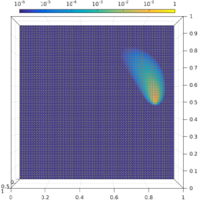
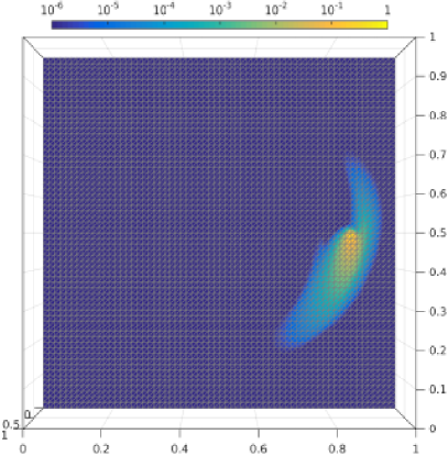
Figure 3: Top view on the modulus of (ideal) test basis functions $(1-\mathcal{C})\lambda_{z}$ with logarithmic color scale. The underlying data are $\epsilon=2^{-8}$ and $b_{1}$ (left) and $b_{2}$ (right) from (4.14).

Figure 3 displays the modified basis functions $(1-\mathcal{C})\lambda_{z}$ for the following non-constant vector fields

$$b_{1}(x)=5\begin{pmatrix}x_{2}-0.5\\ 0.5-x_{1}\end{pmatrix}\;\text{and}\;\;b_{2}(x)=\left(2\left(\left\lceil x-\begin{pmatrix}0.5\\ 0.5\end{pmatrix}\right\rceil-1\right)\operatorname{mod}2\right)b_{1}(x),$$ (4.14)

where $\lceil r\rceil:=\min\{k\in\mathbb{N}\mid k\geq r\}$ denotes the ceiling function. One observes that the decay is directed along $b$.

5 LOD method and error analysis

Based on the results above, we conclude that the energy norm of $\mathcal{C}_{T}v$ decreases very fast outside of a local region around $T$ for any $v\in V_{H}$. Therefore, a localization process is feasible to reduce the computational costs of the ideal method but maintain a good accuracy. In this section, we want to localize the corrector problems (3.2). To this end, instead of solving them on the global domain $\Omega$, we obtain a good approximation of those correctors by solving a local problem on $\Omega_{T,\ell,b}$.

Firstly, let us introduce some notations. In the following, we will denote $R_{H}=\mathrm{Ker}I_{H}$, and $R_{H}(\Omega_{T,\ell,b})=\{w\in R_{H},\text{ and }w=0\text{ in }\Omega\setminus\Omega_{T,\ell,b}\}$. Recall the local bilinear form $a_{\omega}$ defined in (4.1). The localized element corrector $\mathcal{C}_{T,\ell}:V_{H}\rightarrow R_{H}(\Omega_{T,\ell,b})$ is defined as follows: given $v_{H}\in V_{H}$, let $\mathcal{C}_{T,\ell}v_{H}\in R_{H}(\Omega_{T,\ell,b})$ satisfy

$$a_{\Omega_{T,\ell,b}}(w,\mathcal{C}_{T,\ell}v_{H})=a_{T}(w,v_{H})\qquad\text{for all }w\in R_{H}(\Omega_{T,\ell,b}).$$ (5.1)

Then we denote $\mathcal{C}_{\ell}:=\sum\limits_{T\in\mathcal{T}_{H}}\mathcal{C}_{T,\ell}$; see Figure 4 for an illustration of the localized correctors $\mathcal{C}_{\ell}\lambda_{z}$ and the corresponding localized test basis.

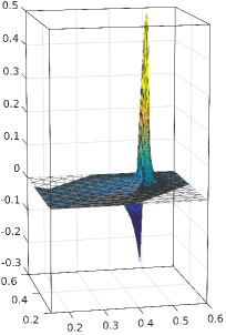
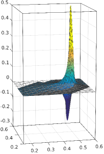
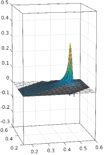
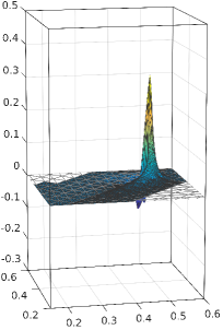
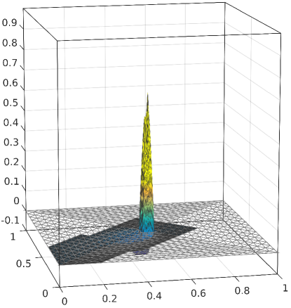
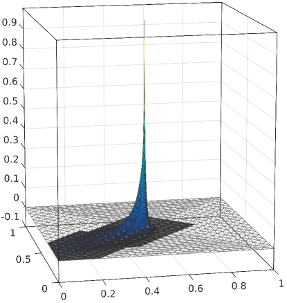
Figure 4: Localized element correctors $\mathcal{C}_{T,\ell}\lambda_{z}$ for $\ell=2$ and all four elements $T$ adjacent to the vertex $z=[0.5,0.5]$ (top), localized nodal corrector $\mathcal{C}_{\ell}\lambda_{z}=\sum_{T\ni z}\mathcal{C}_{T,\ell}\lambda_{z}$ (bottom left) and corresponding test basis function $(1-\mathcal{C}_{\ell})\lambda_{z}$ (bottom right). The underlying data is $b=[\cos(0.7),\sin(0.7)]$ and $\epsilon=2^{-7}$. The computations have been performed by standard linear finite elements on local fine meshes of width $h=2^{-8}$. See Fig. 1 for a comparison with the ideal global corrector and basis.

In the following lemma, we will show that $\mathcal{C}_{T,\ell}$ is a good approximation of $\mathcal{C}_{T}$ provided that the local patches $\Omega_{T,\ell,b}$ are sufficiently large. For the ease of presentation, we denote the mesh Péclet number $\mathrm{Pe}_{H,b,\epsilon}\,$ of $\mathcal{T}_{H}$ by

$$\mathrm{Pe}_{H,b,\epsilon}\,:=H\|b\|_{L^{\infty}(\Omega)}/\epsilon.$$ (5.2)

Recall the definition of $\beta$ from (4.6).

Lemma 5.1.

Given $v\in V_{H}$ and $\ell\in\mathbb{N}_{+}$, it holds that

$$\left|\mathcal{C}_{T}v-\mathcal{C}_{T,\ell}v\right|_{H^{1}\left(\Omega\right)}\lesssim\left(1+\mathrm{Pe}_{H,b,\epsilon}\,C_{I_{H}}\big{(}\tfrac{H}{h}\big{)}\right)^{2}(C_{I_{H}}\big{(}\tfrac{H}{h}\big{)}+1)\beta^{\ell-1}\left|v\right|_{H^{1}\left(T\right)}.$$ (5.3)

Proof.

Denote $e_{T,\ell}:=\mathcal{C}_{T}v-\mathcal{C}_{T,\ell}v$. In view of $R_{H}(\Omega_{T,\ell,b})\subset R_{H}$, the definitions of the correctors in (5.1) and (3.2) and the orthogonality of Petrov-Galerkin type, lead to

$$\epsilon\left|e_{T,\ell}\right|_{H^{1}\left(\Omega\right)}^{2}=a(e_{T,\ell},e_{T,\ell})=a(e_{T,\ell}-w,e_{T,\ell})\quad\text{ for all }w\in R_{H}(\Omega_{T,\ell,b}).$$

Since $I_{H}(e_{T,\ell})=0$, Hölder’s inequality, and the approximation property (3.1) of $I_{H}$ imply

$$\left|e_{T,\ell}\right|_{H^{1}\left(\Omega\right)}^{2}\leq\left(1+\mathrm{Pe}_{H,b,\epsilon}\,C_{I_{H}}\big{(}\tfrac{H}{h}\big{)}\right)\left|e_{T,\ell}\right|_{H^{1}\left(\Omega\right)}\left|e_{T,\ell}-w\right|_{H^{1}\left(\Omega\right)}.$$

Since $w\in R_{H}(\Omega_{T,\ell,b})$ is arbitrary, we arrive at

$$\left|e_{T,\ell}\right|_{H^{1}\left(\Omega\right)}\leq\left(1+\mathrm{Pe}_{H,b,\epsilon}\,C_{I_{H}}\big{(}\tfrac{H}{h}\big{)}\right)\left|\mathcal{C}_{T}v-w\right|_{H^{1}\left(\Omega\right)}.$$ (5.4)

In the following, we construct a specific $w\in R_{H}(\Omega_{T,\ell,b})$ to control the term $\left|\mathcal{C}_{T}v-w\right|_{H^{1}\left(\Omega\right)}$. Let $\eta$ denote the cut-off function from the proof of Theorem 4.1, such that $\eta|_{S_{T,\ell-1,b}}=0$ and $\eta|_{\Omega\setminus S_{T,\ell,b}}=1$. Note that $S_{T,\ell,b}\subset\Omega_{T,\ell,b}$ and therefore $\mu:=1-\eta$ satisfies $\mu|_{\Omega\setminus\Omega_{T,\ell,b}}=0$. In addition, $\mu$ is bounded between 0 and 1 and satisfies the Lipschitz continuity

$$\left\|\nabla\mu\right\|_{L^{\infty}\left(\Omega\right)}\leq 2H^{-1}.$$ (5.5)

Define $w=\mu\mathcal{C}_{T}v$, then $w\in R_{H}(\Omega_{T,\ell,b})$. Since $\mathcal{C}_{T}v\in R_{H}$, the fact that $0\leq\mu\leq 1$ and (5.5) lead as in the proof of Theorem 4.1 to

$$\left|\mathcal{C}_{T}v-w\right|_{H^{1}\left(\Omega\right)} =\left|\mathcal{C}_{T}v-\mu\mathcal{C}_{T}v\right|_{H^{1}\left(\Omega\setminus S_{T,\ell-1,b}\right)}$$

$$\leq 2(C_{I_{H}}\big{(}\tfrac{H}{h}\big{)}+1)\left|\mathcal{C}_{T}v\right|_{H^{1}\left(\Omega\setminus S_{T,\ell-1,b}\right)}.$$

Theorem 4.1 then implies

$$\left|\mathcal{C}_{T}v-w\right|_{H^{1}\left(\Omega\right)} \lesssim(C_{I_{H}}\big{(}\tfrac{H}{h}\big{)}+1)\beta^{\ell-1}\left|\mathcal{C}_{T}v\right|_{H^{1}\left(\Omega\right)}.$$

The combination with (5.4) implies

$$\left|\mathcal{C}_{T}v-\mathcal{C}_{T,\ell}v\right|_{H^{1}\left(\Omega\right)}\lesssim\left(1+\mathrm{Pe}_{H,b,\epsilon}\,C_{I_{H}}\big{(}\tfrac{H}{h}\big{)}\right)(C_{I_{H}}\big{(}\tfrac{H}{h}\big{)}+1)\beta^{\ell-1}\left|\mathcal{C}_{T}v\right|_{H^{1}\left(\Omega\right)}.$$

In the end, we show the stability of $\mathcal{C}_{T}$ to bound the term $\left|\mathcal{C}_{T}v\right|_{H^{1}\left(\Omega\right)}$. Since $I_{H}(\mathcal{C}_{T}v)=0$, the stability of $\mathcal{C}_{T}$ follows from

$$\epsilon\left|\mathcal{C}_{T}v\right|_{H^{1}\left(\Omega\right)}^{2} =a(\mathcal{C}_{T}v,\mathcal{C}_{T}v)=a_{T}(\mathcal{C}_{T}v,v)$$

$$\leq\epsilon\left|\mathcal{C}_{T}v\right|_{H^{1}\left(\Omega\right)}\left|v\right|_{H^{1}\left(T\right)}+\|b\|_{L^{\infty}(T)}\left|v\right|_{H^{1}\left(T\right)}\left\|\mathcal{C}_{T}v\right\|_{L^{2}\left(\Omega\right)}$$

$$\leq\left(\epsilon+H\|b\|_{L^{\infty}(T)}C_{I_{H}}\big{(}\tfrac{H}{h}\big{)}\right)\left|\mathcal{C}_{T}v\right|_{H^{1}\left(\Omega\right)}\left|v\right|_{H^{1}\left(T\right)},$$

where the definition of the element corrector in (5.1) implies the second equality and the approximation property (3.1) leads to the last inequality. This proves the assertion. ∎

The following theorem assembles the local estimates from Lemma 5.1 to derive an estimate for the global corrector.

Theorem 5.2.

Given $v\in V_{H}$ and $\ell\in\mathbb{N}_{+}$, it holds that

$$\left|\mathcal{C}v-\mathcal{C}_{\ell}v\right|_{H^{1}\left(\Omega\right)}\lesssim C(H,h,\epsilon,b,\ell)\beta^{\ell-1}\left|v\right|_{H^{1}\left(\Omega\right)}$$ (5.6)

with

$$C(H,h,\epsilon,b,\ell) :=\left(1+\mathrm{Pe}_{H,b,\epsilon}\,C_{I_{H}}\big{(}\tfrac{H}{h}\big{)}\right)^{2}(C_{I_{H}}\big{(}\tfrac{H}{h}\big{)}+1)$$ (5.7)

$$\qquad\times\left(1+2C_{I_{H}}\big{(}\tfrac{H}{h}\big{)}+\mathrm{Pe}_{H,b,\epsilon}\,C_{I_{H}}\big{(}\tfrac{H}{h}\big{)}\right)C_{\mathrm{ol},\ell+2}(\epsilon)^{1/2}.$$

Proof.

Set $z:=\mathcal{C}v-\mathcal{C}_{\ell-2}v\in\mathrm{Ker}I_{H}$ and $z_{T}:=\mathcal{C}_{T}v-\mathcal{C}_{T,\ell-2}v$, then $z=\sum\limits_{T\in\mathcal{T}_{H}}z_{T}$. We have

$$\epsilon\left|z\right|_{H^{1}\left(\Omega\right)}^{2}=\sum\limits_{T\in\mathcal{T}_{H}}a(z,z_{T}).$$ (5.8)

We estimate $a(z,z_{T})$ for each coarse element $T\in\mathcal{T}_{H}$. Recall that we defined a cutoff function $\eta$ in the proof of Theorem 4.1. Note that $\Omega_{T,\ell-2,b}\subset S_{T,\ell-1,b}$. By construction, we have $\eta z\in R_{H}(\Omega\setminus S_{T,\ell-1,b})\subset R_{H}(\Omega\setminus\Omega_{T,\ell-2,b})$. Since $\mathcal{C}_{T,\ell-2}v|_{\Omega\setminus\Omega_{T,\ell-2,b}}=0$, this implies

$$a(\eta z,z_{T})=a(\eta z,\mathcal{C}_{T}v).$$

Furthermore, notice that $\eta z\in\mathrm{ker}(I_{H})$, which combined with (4.2) yields

$$a(\eta z,\mathcal{C}_{T}v)=a_{T}(\eta z,v)=0.$$

As a consequence, we obtain

$$a(z,z_{T})=a(\eta z,z_{T})+a((1-\eta)z,z_{T})=a((1-\eta)z,z_{T}).$$

In the following, we will bound the term $a((1-\eta)z,z_{T})$. Recall from the proof of Theorem 4.1 that $(1-\eta)|_{\Omega\setminus S_{T,\ell,b}}=0$, $\|\nabla(1-\eta)\|_{L^{\infty}(\Omega)}\leq 2H^{-1}$ and $\|(1-\eta)\|_{L^{\infty}(\Omega)}\leq 1$. Taking into account that $I_{H}(z)=I_{H}(z_{T})=0$, the stability of the projector $I_{H}$ from (3.1), therefore, leads to

$$a((1-\eta)z,z_{T})$$

$$\qquad\leq\epsilon\left|(1-\eta)z\right|_{H^{1}\left(S_{T,\ell,b}\right)}\left|z_{T}\right|_{H^{1}\left(S_{T,\ell,b}\right)}+\|b\|_{L^{\infty}(\Omega)}\left\|z\right\|_{L^{2}\left(S_{T,\ell,b}\right)}\left|z_{T}\right|_{H^{1}\left(S_{T,\ell,b}\right)}$$

$$\qquad\leq\left(\epsilon(1+2C_{I_{H}}\big{(}\tfrac{H}{h}\big{)})+\|b\|_{L^{\infty}(\Omega)}HC_{I_{H}}\big{(}\tfrac{H}{h}\big{)}\right)\left|z\right|_{H^{1}\left(S_{T,\ell,b}\right)}\left|z_{T}\right|_{H^{1}\left(S_{T,\ell,b}\right)}.$$

Since $S_{T,\ell,b}\subset\Omega_{T,\ell,b}$, the combination with (5.8) and the application of a discrete Cauchy-Schwarz inequality yields

$$\left|z\right|_{H^{1}\left(\Omega\right)}^{2} \leq\left(1+2C_{I_{H}}\big{(}\tfrac{H}{h}\big{)}+\mathrm{Pe}_{H,b,\epsilon}\,C_{I_{H}}\big{(}\tfrac{H}{h}\big{)}\right)\sum\limits_{T\in\mathcal{T}_{H}}\left|z\right|_{H^{1}\left(S_{T,\ell,b}\right)}\left|z_{T}\right|_{H^{1}\left(S_{T,\ell,b}\right)}$$

$$\leq\left(1+2C_{I_{H}}\big{(}\tfrac{H}{h}\big{)}+\mathrm{Pe}_{H,b,\epsilon}\,C_{I_{H}}\big{(}\tfrac{H}{h}\big{)}\right)$$

$$\qquad\qquad\qquad\times\Bigg{(}\sum\limits_{T\in\mathcal{T}_{H}}\left|z\right|_{H^{1}\left(\Omega_{T,\ell,b}\right)}^{2}\Bigg{)}^{1/2}\Bigg{(}\sum\limits_{T\in\mathcal{T}_{H}}\left|z_{T}\right|_{H^{1}\left(S_{T,\ell,b}\right)}^{2}\Bigg{)}^{1/2}.$$

Lemma 5.1 implies

$$\Bigg{(}\sum\limits_{T\in\mathcal{T}_{H}}\left|z_{T}\right|_{H^{1}\left(S_{T,\ell,b}\right)}^{2}\Bigg{)}^{1/2}$$

$$\qquad\qquad\lesssim\left(1+\mathrm{Pe}_{H,b,\epsilon}\,C_{I_{H}}\big{(}\tfrac{H}{h}\big{)}\right)^{2}(C_{I_{H}}\big{(}\tfrac{H}{h}\big{)}+1)\beta^{\ell-3}\left|v\right|_{H^{1}\left(\Omega\right)},$$

while the bounded overlap of the patches from (4.4) implies

$$\Bigg{(}\sum\limits_{T\in\mathcal{T}_{H}}\left|z\right|_{H^{1}\left(\Omega_{T,\ell,b}\right)}^{2}\Bigg{)}^{1/2}\leq C_{\mathrm{ol},\ell}(\epsilon)^{1/2}\left|z\right|_{H^{1}\left(\Omega\right)}.$$

In the end, the combination of the previous displayed inequalities and the shift $\ell\mapsto\ell+2$ shows the assertion. ∎

Now we are ready to define the localized multiscale test space as

$$W_{H,\ell}=(1-\mathcal{C}_{\ell})V_{H}.$$

The Petrov-Galerkin method for the approximation of (2.5) based on the trial-test pairing $(V_{H},W_{H,\ell})$ defined above seeks $u_{H,\ell}\in V_{H}$ satisfying

$$a(u_{H,\ell},w_{H,\ell})=\langle f,w_{H,\ell}\rangle_{H^{-1}(\Omega)\times H^{1}_{0}(\Omega)}\qquad\text{for all }w_{H,\ell}\in W_{H,\ell}.$$ (5.9)

Lemma 5.3 (Inf-sup stability).

If $\ell$ is sufficiently large, i.e., the oversampling condition

$$\ell\gtrsim\frac{1+\lvert\log(C_{I_{H}}\big{(}\tfrac{H}{h}\big{)})\rvert+\lvert\log(C(H,h,\epsilon,b,\ell)\rvert+\lvert\log(1+C_{I_{H}}\big{(}\tfrac{H}{h}\big{)}+\mathrm{Pe}_{H,b,\epsilon}\,C_{I_{H}}\big{(}\tfrac{H}{h}\big{)}^{2})\rvert}{\lvert\log(4C_{I_{H}}\big{(}\tfrac{H}{h}\big{)}+3C_{I_{H}}\big{(}\tfrac{H}{h}\big{)}^{2})-\log(1+4C_{I_{H}}\big{(}\tfrac{H}{h}\big{)}+3C_{I_{H}}\big{(}\tfrac{H}{h}\big{)}^{2})\rvert}$$ (5.10)

is satisfied, then the Petrov-Galerkin method (5.9) is inf-sup stable and

$$\inf\limits_{w_{H,\ell}\in W_{H,\ell}\setminus\{0\}}\sup\limits_{u_{H}\in V_{H}\setminus\{0\}}\frac{a(u_{H},w_{H,\ell})}{\left|u_{H}\right|_{H^{1}\left(\Omega\right)}\left|w_{H,\ell}\right|_{H^{1}\left(\Omega\right)}}\gtrsim\frac{\epsilon}{C_{I_{H}}\big{(}\tfrac{H}{h}\big{)}}.$$ (5.11)

Remark 5.4.

If $H/h=1/\epsilon$ and $\lvert b\rvert=1$, then (5.10) reads

$$\ell\gtrsim(\log(\epsilon))^{2},$$

i.e., the local patch size $\ell$ depends on $\log(\epsilon)$ algebraically.

Remark 5.5.

Since the dimension of $V_{H}$ equals the dimension of $W_{H,\ell}$, the reverse inf-sup condition

$$\inf_{u_{H}\in V_{H}\setminus\{0\}}\sup_{w_{H,\ell}\in W_{H,\ell}\setminus\{0\}}\frac{a(u_{H},w_{H,\ell})}{\left|u_{H}\right|_{H^{1}\left(\Omega\right)}\left|w_{H,\ell}\right|_{H^{1}\left(\Omega\right)}}\gtrsim\frac{\epsilon}{C_{I_{H}}\big{(}\tfrac{H}{h}\big{)}}.$$ (5.12)

follows from Lemma 5.3.

Proof of Lemma 5.3.

Let $w_{H,\ell}\in W_{H,\ell}$, and set $w_{H}=(1-\mathcal{C})I_{H}w_{H,\ell}\in W_{H}$. By Lemma 3.3, there exists $u_{H}\in V_{H}$, s.t.,

$$a(u_{H},w_{H})\geq\frac{\epsilon}{C_{I_{H}}\big{(}\tfrac{H}{h}\big{)}}\left|u_{H}\right|_{H^{1}\left(\Omega\right)}\left|w_{H}\right|_{H^{1}\left(\Omega\right)}.$$ (5.13)

Taking into account that $w_{H,\ell}=I_{H}w_{H,\ell}-\mathcal{C}_{\ell}I_{H}w_{H,\ell}$, we arrive at $w_{H}-w_{H,\ell}=(\mathcal{C}_{\ell}-\mathcal{C})I_{H}w_{H,\ell}$. As a consequence, Theorem 5.2 together with the stability of $I_{H}$ from (3.1) implies

$$\left|w_{H}-w_{H,\ell}\right|_{H^{1}\left(\Omega\right)} \leq\tilde{C}C(H,h,\epsilon,b,\ell)\beta^{\ell-1}\left|I_{H}w_{H,\ell}\right|_{H^{1}\left(\Omega\right)}$$

$$\leq\tilde{C}C(H,h,\epsilon,b,\ell)C_{I_{H}}\big{(}\tfrac{H}{h}\big{)}\beta^{\ell-1}\left|w_{H,\ell}\right|_{H^{1}\left(\Omega\right)}.$$

Here, $\tilde{C}$ denotes the constant hidden in $\lesssim$ in Theorem 5.2, which is independent of $H$, $h$ or $\epsilon$. The combination with a triangle inequality leads to

$$\left|w_{H}\right|_{H^{1}\left(\Omega\right)} \geq\left|w_{H,\ell}\right|_{H^{1}\left(\Omega\right)}-\left|w_{h}-w_{H,\ell}\right|_{H^{1}\left(\Omega\right)}$$

$$\geq(1-\tilde{C}C(H,h,\epsilon,b,\ell)C_{I_{H}}\big{(}\tfrac{H}{h}\big{)}\beta^{\ell-1})\left|w_{H,\ell}\right|_{H^{1}\left(\Omega\right)}.$$

Since $I_{H}(w_{H,\ell}-w_{H})=0$, i.e., $w_{H,\ell}-w_{H}\in R_{H}$, this leads to

$$\lvert a(u_{H},w_{H,\ell}-w_{H})\rvert \leq(\epsilon+\|b\|_{L^{\infty}(\Omega)}HC_{I_{H}}\big{(}\tfrac{H}{h}\big{)})\left|u_{H}\right|_{H^{1}\left(\Omega\right)}\left|w_{H,\ell}-w_{H}\right|_{H^{1}\left(\Omega\right)}$$

$$=\epsilon(1+\text{Pe}_{H,b,\epsilon}C_{I_{H}}\big{(}\tfrac{H}{h}\big{)})\left|u_{H}\right|_{H^{1}\left(\Omega\right)}\left|w_{H,\ell}-w_{H}\right|_{H^{1}\left(\Omega\right)}.$$

The combination of the above displayed inequalities results in

$$a(u_{H},w_{H,\ell})=a(u_{H},w_{H})+a(u_{H},w_{H,\ell}-w_{H})$$

$$\geq\frac{\epsilon}{C_{I_{H}}\big{(}\tfrac{H}{h}\big{)}}(1-\tilde{C}C(H,h,\epsilon,b,\ell)C_{I_{H}}\big{(}\tfrac{H}{h}\big{)}\beta^{\ell-1})\left|u_{H}\right|_{H^{1}\left(\Omega\right)}\left|w_{H,\ell}\right|_{H^{1}\left(\Omega\right)}$$

$$\qquad-\epsilon(1+\mathrm{Pe}_{H,b,\epsilon}\,C_{I_{H}}\big{(}\tfrac{H}{h}\big{)})C(H,h,\epsilon,b,\ell)\tilde{C}C_{I_{H}}\big{(}\tfrac{H}{h}\big{)}\beta^{\ell-1}\left|u_{H}\right|_{H^{1}\left(\Omega\right)}\left|w_{H,\ell}\right|_{H^{1}\left(\Omega\right)}.$$

Recall the definition of $\beta$ from (4.6). If $\ell$ satisfies (5.10), then we obtain (5.11). ∎

We are ready to estimate the error $\left|u_{H}-u_{H,\ell}\right|_{H^{1}\left(\Omega\right)}$ coming from the localization.

Lemma 5.6.

Let $\ell$ satisfy (5.10). Then

$$\left|u_{H}-u_{H,\ell}\right|_{H^{1}\left(\Omega\right)} \lesssim C_{I_{H}}\big{(}\tfrac{H}{h}\big{)}^{2}C(H,h,\epsilon,b,\ell)(1+\mathrm{Pe}_{H,b,\epsilon}\,C_{I_{H}}\big{(}\tfrac{H}{h}\big{)})$$ (5.14)

$$\qquad\qquad\qquad\qquad\qquad\times\beta^{\ell-1}\left|u_{h}-u_{H}\right|_{H^{1}\left(\Omega\right)}.$$

Proof.

Notice that $u_{H}-u_{H,\ell}\in V_{H}$ is a coarse finite element function. Therefore, the inf-sup condition (5.12) guarantees the existence of $w_{H,\ell}\in W_{H,\ell}$ with

$$\left|u_{H}-u_{H,\ell}\right|_{H^{1}\left(\Omega\right)}\lesssim\frac{C_{I_{H}}\big{(}\tfrac{H}{h}\big{)}}{\epsilon}\frac{a(u_{H}-u_{H,\ell},w_{H,\ell})}{\left|w_{H,\ell}\right|_{H^{1}\left(\Omega\right)}}.$$

In view of $w_{H,\ell}\in W_{H,\ell}\subset V_{h}$, the standard Galerkin problem (2.5) and the VMS (5.9) imply

$$a(u_{H}-u_{H,\ell},w_{H,\ell})=a(u_{H}-u_{h},w_{H,\ell}).$$

Define $w_{H}:=I_{H}w_{H,\ell}-\mathcal{C}(I_{H}w_{H,\ell})\in W_{H}\subset V_{h}$. Together with the orthogonality of Petrov-Galerkin type, we obtain

$$a(u_{H}-u_{h},w_{H,\ell})=a(u_{H}-u_{h},w_{H,\ell}-w_{H}).$$

Taking into account that $w_{H,\ell}-w_{H}=\mathcal{C}_{\ell}I_{H}w_{H,\ell}-\mathcal{C}I_{H}w_{H,\ell}$, the combination with a Cauchy inequality, $w_{H,\ell}-w_{H}\in\mathrm{ker}(I_{H})$ and an application of Theorem 5.2 lead to

$$a(u_{H}-u_{h},w_{H,\ell}-w_{H})$$

$$\qquad\lesssim(\epsilon+\|b\|_{L^{\infty}(\Omega)}HC_{I_{H}}\big{(}\tfrac{H}{h}\big{)})C(H,h,\epsilon,b,\ell)\beta^{\ell-1}\left|I_{H}w_{H,\ell}\right|_{H^{1}\left(\Omega\right)}\left|u_{h}-u_{H}\right|_{H^{1}\left(\Omega\right)}.$$

The stability of $I_{H}$ from (3.1) implies the assertion. ∎

Lemma 5.6 allows bounding the error for the localized VMS in the following manner.

Theorem 5.7 (global error estimate for localized VMS).

Let $\ell$ satisfy (5.10), then

$$\left|u_{h}-u_{H,\ell}\right|_{H^{1}\left(\Omega\right)} \lesssim\left(C_{I_{H}}\big{(}\tfrac{H}{h}\big{)}+C_{I_{H}}\big{(}\tfrac{H}{h}\big{)}^{3}C(H,h,\epsilon,b,\ell)(1+\mathrm{Pe}_{H,b,\epsilon}\,C_{I_{H}}\big{(}\tfrac{H}{h}\big{)})\beta^{\ell-1}\right)$$

$$\qquad\qquad\qquad\qquad\qquad\qquad\qquad\qquad\times\min_{v_{H}\in V_{H}}\left|u_{h}-v_{H}\right|_{H^{1}\left(\Omega\right)}$$

with the constant $(C(H,h,\epsilon,b,\ell)$ from (5.7).

Proof.

The proof follows directly from a triangle inequality, Proposition 3.1, and Lemma 5.6. ∎

Although Theorem 5.7 provides a best-approximation result, the assertion still depends on $\epsilon$, which is hidden in the best-approximation $\min_{v_{H}\in V_{H}}\left|u_{h}-v_{H}\right|_{H^{1}\left(\Omega\right)}$. The locality in the error bound of the ideal method from Proposition 3.1 transfers to the VMS defined in (5.9) and results in the local error bound in the following theorem. Note that the error from the localization still depends on the mesh Péclet number of $\mathcal{T}_{H}$ and still contains the best-approximation error on the whole domain. Nevertheless, this ill-behaved terms are weighted by the exponentially decaying term $\beta^{\ell-1}$, where $\beta$ is bounded above from 1.

Theorem 5.8 (local error estimate for localized VMS).

Let $\ell$ satisfy (5.10). Then for any $\mathcal{K}\subset\mathcal{T}$ and $\omega:=\cup\mathcal{K}$, it holds that

$$\left|u_{h}-u_{H,\ell}\right|_{H^{1}\left(\omega\right)}\lesssim C_{I_{H}}\big{(}\tfrac{H}{h}\big{)}\min_{v_{H}\in V_{H}}\left|u_{h}-v_{H}\right|_{H^{1}\left(\omega\right)}$$

$$\qquad\quad+C_{I_{H}}\big{(}\tfrac{H}{h}\big{)}^{3}C(H,h,\epsilon,b,\ell)(1+\mathrm{Pe}_{H,b,\epsilon}\,C_{I_{H}}\big{(}\tfrac{H}{h}\big{)})\beta^{\ell-1}\min_{v_{H}\in V_{H}}\left|u_{h}-v_{H}\right|_{H^{1}\left(\Omega\right)}.$$

Remark 5.9 (complexity).

The problem (5.9) on the coarse scale consists of $\mathcal{O}(1/H^{2})$ degrees of freedom (DOFs). Corresponding to each of those DOFs, one localized corrector problem (5.1) has to be solved, which relates to $\mathcal{O}(\ell^{2}H^{3}/(h^{2}\epsilon))$ DOFs in the worst case scenario. If the mesh is structured, the number of corrector problems that have to be solved can be reduced to $\mathcal{O}(\ell H/\epsilon)$, cf. [11].

6 Numerical experiment

In this section, we present one simple numerical test to illustrate the theoretical convergence results of the localized method proposed in (5.9). We take $\Omega=(0,1)\times(0,1)$, the velocity field $b=(\cos(0.7),\sin(0.7))^{\top}$, the volume force $f\equiv 1$ and $\epsilon=2^{-7}$. The reference solution $u_{h}$ is obtained through (2.5) by taking $h=\sqrt{2}\,2^{-8}$.

We will compare our approache with SUPG. Let us briefly review the SUPG model to (1.1) [10]. Let $(\bullet,\bullet)_{T}:=(\bullet,\bullet)_{L^{2}(T)}$ denote the $L^{2}$ scalar product over a triangle $T\in\mathcal{T}_{H}$. Then SUPG seeks $u_{H}\in V_{H}$ such that

$$B_{\mathrm{SUPG}}(u_{H}^{\mathrm{SUPG}},v_{H})=F_{\mathrm{SUPG}}(v_{H})\qquad\text{for all }v_{H}\in V_{H}$$ (6.1)

with

$$B_{\mathrm{SUPG}}(u_{H}^{\mathrm{SUPG}},v_{H})=a(u_{H}^{\mathrm{SUPG}},v_{H})+\delta_{\mathrm{SUPG}}\sum\limits_{T\in\mathcal{T}_{H}}(b\cdot\nabla u_{H}^{\mathrm{SUPG}},b\cdot\nabla v_{H})_{T}$$

and

$$F_{\mathrm{SUPG}}(v_{H})=\langle f,v_{H}\rangle_{H^{-1}(\Omega)\times H^{1}_{0}(\Omega)}+\delta_{\mathrm{SUPG}}\sum\limits_{k\in\mathcal{T}_{H}}(f,b\cdot\nabla v_{H})_{T}.$$

Here, $\delta_{\mathrm{SUPG}}$ indicates the stability parameter, and we choose

$$\delta_{\mathrm{SUPG}}=\frac{H}{\sqrt{8}\max(\epsilon,H/\sqrt{2})}$$

in our numerical test.

The reference solution from (2.5) and the coarse scale solution from (5.9) and the SUPG solution from (6.1) with $H=\sqrt{2}\,2^{-4}$ are depicted in Figure 5. One can observe that the classical FEM approximation with $H=\sqrt{2}\,2^{-4}$ is not stable around the boundary layers (i.e. the top and right boundaries) and shows spurious oscillations, and thus fails to provide a reliable solution. Nevertheless, both the SUPG method and the ideal method are stable and generate an accurate solution. We display the solutions for fixed $y=0.75$ to illustrate the stability and accuracy of the VMS method in Figure 6. We observe large oscillations in the coarse scale solution obtained through classical FEM when $x$ approaches 1, while the SUPG and the VMS method yield reliable solutions. The smearing is restricted to one layer of elements around the boundary. We can also conclude that the SUPG and the VMS method reproduce the reference solution away from $x=1$ and the latter shows slightly less smearing. We want to highlight that the localization parameter is $\ell=1$ for the VMS method in this example.

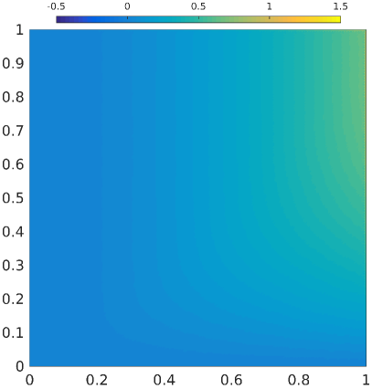
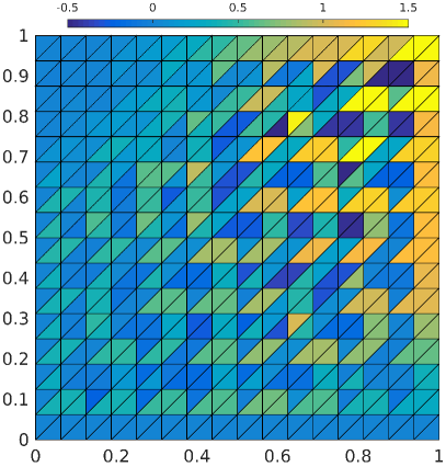
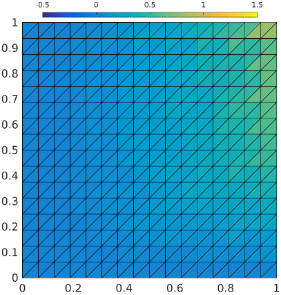
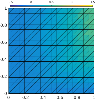
Figure 5: Reference solution (top left), classical FEM approximation (top right), SUPG approximation (bottom left), and multiscale approximation for $\ell=1$ (bottom right) for $\epsilon=2^{-7}$ and $H=\sqrt{2}\,2^{-4}$.

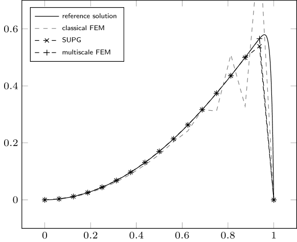
Figure 6: Reference solution, classical FEM, SUPG and multiscale approximation for $\ell=1$ at the line $y=0.75$ on a mesh with mesh-size $H=\sqrt{2}\,2^{-4}$ for $\epsilon=2^{-7}$.

Tables 1 and 2 display the errors between the localized solutions (5.9) and the reference solution $u_{h}$ under various coarse mesh-sizes $H$ and localization parameters $\ell$. We observe an optimal convergence rate of $\mathcal{O}(H)$ in Table 1 for the error in the $H^{1}$ semi norm in the domain $[0,0.75]\times[0,0.75]$ away from the boundary layers, and an optimal convergence rate of $\mathcal{O}(H^{2})$ in Table 2 for the global error in the $L^{2}$ norm. Although Theorem 5.8 guarantees optimality only under the assumption that $\ell$ is large enough in the sense of (5.10), the numerical experiment demonstrates that $\ell=1$ is sufficient for an accurate solution, which implies a huge potentially computational reduction.

The convergence rate for $u_{H,1}$ with various $\epsilon$ in a range from $2^{-5}$ to $2^{-8}$ is shown in Figures 7 and 8. The error is stable and of order $\mathcal{O}(H)$ with respect to the $H^{1}$ semi norm in a region away from boundary layers and of order $\mathcal{O}(H^{2})$ in the global $L^{2}$ norm with a preasymptotic effect for smaller values of $\epsilon$. For comparison, the nodal interpolation error (i.e. the error from the ideal method) in the global $L^{2}$ norm is depicted, which agrees with $\left\|u_{h}-u_{H,1}\right\|_{L^{2}(\Omega)}$ very well. This justifies the fast convergence of the localized method with respect to the localization parameter $\ell$ for all of the considered values of $\epsilon$.

	$\ell=1$	$\ell=2$	$\ell=3$	$\ell=4$	$\ell=5$	$\ell=6$
$H=\sqrt{2}2^{-3}$	5.14e-02	5.14e-02	5.14e-02	5.14e-02	5.14e-02	5.14e-02
$H=\sqrt{2}2^{-4}$	2.57e-02	2.57e-02	2.57e-02	2.57e-02	2.57e-02	2.57e-02
$H=\sqrt{2}2^{-5}$	1.27e-02	1.27e-02	1.27e-02	1.27e-02	1.27e-02	1.27e-02
$H=\sqrt{2}2^{-6}$	6.23e-03	6.23e-03	6.23e-03	6.23e-03	6.23e-03	6.23e-03

Table 1: The error $\|\nabla(u_{h}-u_{H,\ell})\|_{L^{2}(\Omega_{r})}$ for $\Omega_{r}=[0,0.75]\times[0,0.75]$ for different localization parameters $\ell$ and mesh-sizes $H$ for $\epsilon=2^{-7}$.

	$\ell=1$	$\ell=2$	$\ell=3$	$\ell=4$	$\ell=5$	$\ell=6$
$H=0.17678$	9.45e-02	9.45e-02	9.45e-02	9.45e-02	9.45e-02	9.45e-02
$H=0.088388$	5.34e-02	5.34e-02	5.34e-02	5.34e-02	5.34e-02	5.34e-02
$H=0.044194$	2.31e-02	2.32e-02	2.32e-02	2.32e-02	2.32e-02	2.32e-02
$H=0.022097$	7.25e-03	7.27e-03	7.27e-03	7.27e-03	7.27e-03	7.27e-03

Table 2: The error $\|u_{h}-u_{H,\ell}\|_{L^{2}(\Omega)}$ for different localization parameters $\ell$ and mesh-sizes $H$ for $\epsilon=2^{-7}$.

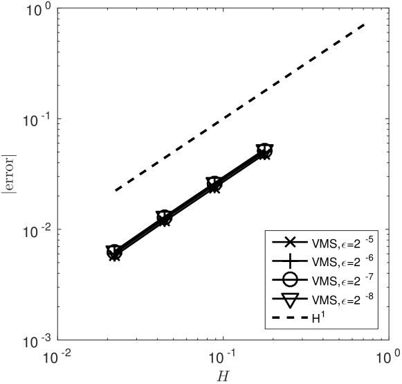
Figure 7: The errors $\|\nabla(u_{h}-u_{H,1})\|_{L^{2}(\Omega_{r})}$ for $\Omega_{r}=[0,0.75]\times[0,0.75]$ for different values of $\epsilon$.

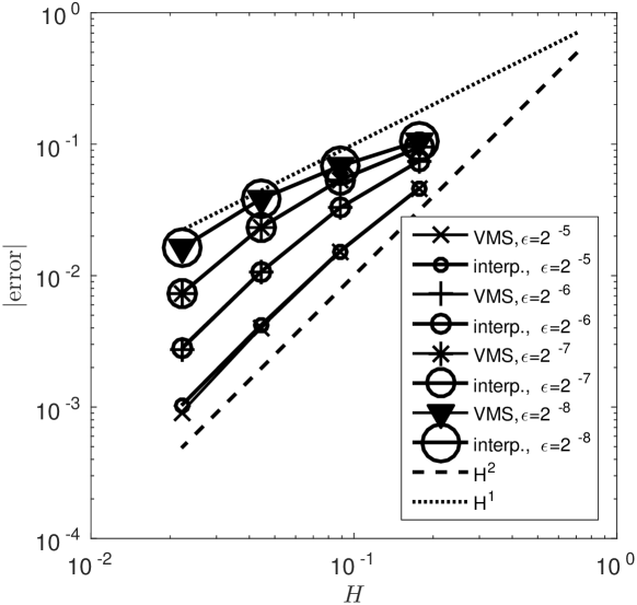
Figure 8: The errors $\|u_{h}-u_{H,1}\|_{L^{2}(\Omega)}$ and $\|u_{h}-I_{H}u_{h}\|_{L^{2}(\Omega)}$ for different values of $\epsilon$.

7 Conclusions

In this paper, a singularly perturbed convection-diffusion equation was considered, and we obtained a stable locally quasi-optimal variational multiscale method based on the nodal interpolation operator. Due to the high complexity involved in solving the global correctors, which account for the main component of the variational multiscale method, a further model reduction was proceeded by localization techniques based on the LOD method. This localization employs local patches which depend on the velocity field $b$ and the singular perturbation parameter $\epsilon$. The error of the localization decays exponentially. We also provided a numerical experiment to illustrate our theoretical results.

The stability constant of the nodal interpolation operator that occurs in the error estimate, depends logarithmically on $H/h$ (and so on $\epsilon$). In the three-dimensional case, this stability estimate depends polynomially on $H/h$. Therefore a generalization of the proposed method to 3D seems to be not reasonable.

The local patches in the localized computation of the corrector depend on $\epsilon$. It is an open question, if this is optimal or if a further reduction or simplification is possible.

References

- [1] G. R. Barrenechea, E. Burman, and F. Karakatsani. Edge-based nonlinear diffusion for finite element approximations of convection–diffusion equations and its relation to algebraic flux-correction schemes. Numerische Mathematik, 2016. Published online.
- [2] F. Brezzi, D. Marini, and E. Süli. Residual-free bubbles for advection-diffusion problems: the general error analysis. Numer. Math., 85(1):31–47, 2000.
- [3] V. M. Calo, E. T. Chung, Y. Efendiev, and W. T. Leung. Multiscale stabilization for convection-dominated diffusion in heterogeneous media. ArXiv e-prints, 2015.
- [4] A. Cangiani and E. Süli. Enhanced residual-free bubble method for convection-diffusion problems. Internat. J. Numer. Methods Fluids, 47(10-11):1307–1313, 2005. 8th ICFD Conference on Numerical Methods for Fluid Dynamics. Part 2.
- [5] A. Cangiani and E. Süli. Enhanced RFB method. Numer. Math., 101(2):273–308, 2005.
- [6] S. Christiansen, T. Halvorsen, and T. Sørensen. Stability of an upwind Petrov-Galerkin discretization of convection diffusion equations. ArXiv e-prints, 2016.
- [7] R. Codina. Stabilization of incompressibility and convection through orthogonal sub-scales in finite element methods. Comput. Methods Appl. Mech. Engrg., 190(13-14):1579–1599, 2000.
- [8] L. Demkowicz, J. Gopalakrishnan, and A. H. Niemi. A class of discontinuous Petrov-Galerkin methods. Part III: Adaptivity. Appl. Numer. Math., 62(4):396–427, 2012.
- [9] D. Elfverson. A discontinuous Galerkin multiscale method for convection-diffustion problems. ArXiv e-prints, 2015.
- [10] L. P. Franca, S. L. Frey, and T. J. Hughes. Stabilized finite element methods: I. Application to the advective-diffusive model. Computer Methods in Applied Mechanics and Engineering, 95(2):253 – 276, 1992.
- [11] D. Gallistl and D. Peterseim. Stable multiscale Petrov-Galerkin finite element method for high frequency acoustic scattering. Comp. Meth. Appl. Mech. Eng., 295:1–17, 2015.
- [12] C. Harder, D. Paredes, and F. Valentin. On a multiscale hybrid-mixed method for advective-reactive dominated problems with heterogeneous coefficients. Multiscale Model. Simul., 13(2):491–518, 2015.
- [13] T. J. R. Hughes and G. Sangalli. Variational multiscale analysis: the fine-scale Green’s function, projection, optimization, localization, and stabilized methods. SIAM J. Numer. Anal., 45(2):539–557, 2007.
- [14] V. John and E. Schmeyer. BAIL 2008 - Boundary and Interior Layers: Proceedings of the International Conference on Boundary and Interior Layers - Computational and Asymptotic Methods, Limerick, July 2008, chapter On Finite Element Methods for 3D Time-Dependent Convection-Diffusion-Reaction Equations with Small Diffusion, pages 173–181. Springer Berlin Heidelberg, Berlin, Heidelberg, 2009.
- [15] M. G. Larson and A. Målqvist. An adaptive variational multiscale method for convection-diffusion problems. Comm. Numer. Methods Engrg., 25(1):65–79, 2009.
- [16] A. Målqvist and D. Peterseim. Localization of elliptic multiscale problems. Math. Comp., 83(290):2583–2603, 2014.
- [17] J. M. Melenk. On the robust exponential convergence of hp finite element methods for problems with boundary layers. IMA Journal of Numerical Analysis, 17(4):577–601, 1997.
- [18] J. M. Melenk. -finite element methods for singular perturbations, volume 1796 of Lecture Notes in Mathematics. Springer-Verlag, Berlin, 2002.
- [19] P. J. Park and T. Y. Hou. Multiscale numerical methods for singularly perturbed convection-diffusion equations. International Journal of Computational Methods, 1(1):17–65, 2004.
- [20] D. Peterseim. Variational multiscale stabilization and the exponential decay of fine-scale correctors. May 2015. To appear.
- [21] D. Peterseim. Eliminating the pollution effect in Helmholtz problems by local subscale correction. Math. Comp., 2016. In press.
- [22] W. Qiu and K. Shi. An HDG method for convection diffusion equation. Journal of Scientific Computing, 66(1):346–357, 2015.
- [23] H. Roos, M. Stynes, and L. Tobiska. Numerical Methods for Singularly Perturbed Differential Equations: Convection-Diffusion and Flow Problems. Springer Series in Computational Mathematics. Springer Berlin Heidelberg, 1996.
- [24] H. Yserentant. On the multilevel splitting of finite element spaces. Numer. Math., 49(4):379–412, 1986.