Qubit state tomography in superconducting circuit via weak measurements

Abstract

The standard method of “measuring” quantum wavefunction is the technique of indirect quantum state tomography. Owing to conceptual novelty and possible advantages, an alternative direct scheme was proposed and demonstrated recently in quantum optics system. In this work we present a study on the direct scheme of measuring qubit state in the circuit QED system, based on weak measurement and weak value concepts. To be applied to generic parameter conditions, our formulation and analysis are carried out for finite strength weak measurement, and in particular beyond the bad-cavity and weak-response limits. The proposed study is accessible to the present state-of-the-art circuit-QED experiments.

I Introduction

In quantum mechanics

, the state of a single system (e.g., a single particle) is described by a wavefunction, which differs drastically from the description in classical mechanics. It is well known that the wavefunction cannot be determined via a single shot measurement WZ82 . Actually, the wavefunction is not a physical quantity, but a knowledge governed by Schrödinger equation and utilized to calculate the real physical quantities by means of statistical average. However, with the advent of quantum information science and technology, experimental manipulation and determination of the wavefunction have become extremely important.

In order to determine the wavefunction, the standard method is based on projective strong measurement where the wavefunction is fully collapsed, and has been termed as quantum state tomography Ris89 ; Smi93 ; Bre97 ; Kwi99 ; Hof09 . In that, one must perform a large set of distinct measurements on many identical copies of the system and reconstruct the state that is most compatible with the measurement results. This tomographic reconstruction of quantum state is considered “indirect” determination, owing to the requirement of post-processing.

An alternative scheme is the so-called “direct” state determination Lun11 ; Lun12 ; Boy13 ; Boy14 , which may have potential applications in quantum information and quantum metrology. This method is based on the idea of sequentially measuring two complementary variables of the system Aha88 ; Ste89 ; Aha90 ; Rit91 ; Wis02 ; Pop04 ; Joh04 ; Wis05 ; Kwi08 ; Jor09 ; Koc11 ; Ste11 . The first measurement is weak, and the second one is strong (projective). The weak measurement (each single one) gets minor information, has gentle disturbance, and does not collapse the state. The second projective measurement plays a role of post-selection. Under this sort of joint measurements, the real and imaginary components of the wavefunction will appear directly on the measurement apparatus, in terms of a shift of the pointer’s position by amount of the weak value (WV) introduced by Aharonov, Albert and Vaidman (AAV) nearly 30 years ago, given by Aha88 ; Aha90

$$A_{w}=\frac{\langle\psi_{f}|\hat{A}|\psi_{i}\rangle}{\langle\psi_{f}|\psi_{i}\rangle}\,,$$ (1)

where $|\psi_{i}\rangle$ and $|\psi_{f}\rangle$ are, respectively, in the context of state tomography, the state to be determined and the one for post-selection. $\hat{A}$ is the weakly observed quantity. The main advantage of this method is that it is free from complicated sets of measurements and computations, manifesting a “directness” of no need of post-processing the average raw signal. For instance, applying this novel approach, recent experiments have been carried out for the direct measurement of photon’s transverse wavefunction (a task not previously realized by any method) Lun11 , and for a full characterization of polarization states of light via direct measurement Boy13 .

In this scheme, weak measurement is at the heart. On the other hand, the superconducting circuit quantum electrodynamics (cQED) system is currently an important platform for performing quantum weak measurement and control studies Bla04 ; Wall04 ; Sid12 ; Dev13 ; Sid13 ; Sid15 . In this work, we present an analysis on the possible direct measurement of qubit state in this system. In order to be applied to generic parameter conditions, our study will be put on finite strength of weak measurement Jor08 ; Li15 . This goes beyond the usual limit of vanishing strength, thus results in a generalized pre- and post-selection (PPS) average, rather than the original AAV WV, as the pointer’s shift of apparatus. To extract the AAV WV from the PPS average (raw signal), we propose to apply the analytic formula derived for the homodyne measurement in circuit QED Li15 . By varying the local oscillator’s (LO) phase, one can easily extract the complex weak value and determine the complex wavefunction, applying a simple iterative algorithm. For the first time, we also obtain analytic result for the PPS average beyond the bad-cavity and weak-response limits, and demonstrate how to reliably determine the qubit state in this regime.

II Methods

II.1 Measurement Current and Rates

The solid-state circuit QED (cQED) system

is originally described by the well-known Jaynes-Cummings (J-C) model Bla04 ; Wall04 . In dispersive regime, i.e., the detuning $\Delta$ between the cavity resonance frequency and the qubit energy being much larger than the J-C coupling strength $g$, the interaction Hamiltonian is reduced as Bla04 ; Wall04

$$H_{\rm int}=\chi a^{\dagger}a\sigma_{z}\,,$$ (2)

where $\chi=g^{2}/\Delta$ is the dispersive coupling, $a^{\dagger}$ and $a$ are the creation and annihilation operators of the cavity photon, and $\sigma_{z}$ is the Pauli operator for the qubit. This type of interaction allows for a homodyne measurement with output current Gam08

$$I(t)=-\sqrt{\Gamma_{ci}(t)}\langle\sigma_{z}\rangle+\xi(t),$$ (3)

where $\xi(t)$ is a Gaussian white noise originated from fundamental quantum-jumps during the measurement. This expression of current was obtained in the absence of qubit rotation and from eliminating the cavity degrees of freedom (the so-called polaron transformation) Gam08 . In a bit more detail, $\Gamma_{ci}(t)$ is the measurement information gain rate given by Gam08

$$\Gamma_{ci}(t)=\kappa|\beta(t)|^{2}\cos^{2}(\varphi-\theta_{\beta})\,,$$ (4)

where $\varphi$ is the local oscillator’s (LO) phase in the homodyne measurement, $\kappa$ is the leaky rate of the cavity photons, and $\beta(t)=\alpha_{2}(t)-\alpha_{1}(t)\equiv|\beta(t)|e^{i\theta_{\beta}}$ with $\alpha_{1}(t)$ and $\alpha_{2}(t)$ being the cavity fields associated with the qubit states $|1\rangle$ and $|2\rangle$, respectively.

In addition to the information gain rate $\Gamma_{ci}$, there exists as well a no-information back-action rate which reads Gam08

$$\Gamma_{ba}(t)=\kappa|\beta(t)|^{2}\sin^{2}(\varphi-\theta_{\beta})\,.$$ (5)

This corresponds to the “realistic” backaction rate discussed in Ref. Kor11 , while $\Gamma_{ci}$ is named “spooky” backaction rate. To understand the physical meaning, let us consider the stochastic evolution of qubit state $c_{1}(t)|1\rangle+c_{2}(t)|2\rangle$, conditioned on measurement records in a single realization. The rate $\Gamma_{ci}$ appearing Eq. (3) is associated with distinguishing the qubit state (information gain), which causes change of the probability amplitudes of $|1\rangle$ and $|2\rangle$. As opposed to this, the rate $\Gamma_{ba}$ is only related to phase fluctuation between $|1\rangle$ and $|2\rangle$ (no probability change). The sum of $\Gamma_{ci}$ and $\Gamma_{ba}$, $\Gamma_{m}=\Gamma_{ci}+\Gamma_{ba}$, gives the total measurement rate. Differing somehow from $\Gamma_{m}$, the overall decoherence rate is given by Gam08

$$\Gamma_{d}(t)=4\chi\mathrm{Im}[\alpha_{1}(t)\alpha^{*}_{2}(t)]\,,$$ (6)

as a result from tracing the cavity degrees of freedom from the whole entangled qubit-cavity state. An interesting point is that $\Gamma_{m}$ is not necessarily equal to $\Gamma_{d}$, owing to ceratin “information loss”. Only for ideal (quantum limited) measurement, $\Gamma_{m}=\Gamma_{d}$ and the single quantum trajectory is a quantum mechanically pure state.

II.2 Quantum Bayesian Rule

Conditioned on the output currents

, Eq. (3), one can faithfully keep track of the stochastic evolution of the qubit state. In order to get analytic expression for the PPS average, rather than the quantum trajectory equation, we apply alternatively the quantum Bayesian rule (BR) Kor99 ; Kor11 ; Li14 ; Li16 . Using the output currents during $(0,t_{m})$, we update first the diagonal elements $\rho_{jj}$ ($j=1,2$) of the qubit state (density matrix) Li14 ; Li16

$$\rho_{jj}(t_{m})=\rho_{jj}(0)\,P_{j}(t_{m})/{\cal N}(t_{m})\,,$$ (7)

where ${\cal N}(t_{m})=\sum_{j=1,2}\rho_{jj}(0)\,P_{j}(t_{m})$. This result simply follows the standard Bayes formula, and the functional distribution of currents reads Li16

$$P_{1(2)}(t_{m})=\exp\left\{-\langle[I(t)-\bar{I}_{1(2)}(t)]^{2}\rangle_{t_{m}}/(2V)\right\}\,,$$ (8)

where $\bar{I}_{1(2)}(t)=\mp\sqrt{\Gamma_{ci}(t)}$ and $\langle\bullet\rangle_{t_{m}}=(t_{m})^{-1}\int^{t_{m}}_{0}dt(\bullet)$, and $V=1/t_{m}$ characterizes the distribution variance. The result of Eq. (8) differs from our usual knowledge. From quite general consideration (central limit theorem), corresponding to $|1\rangle$ and $|2\rangle$, the averaged stochastic current $I_{m}$, $I_{m}=(t_{m})^{-1}\int^{t_{m}}_{0}dtI(t)$, should respectively center at $\bar{I}_{1(2)}=\mp(t_{m})^{-1}\int^{t_{m}}_{0}dt\,\sqrt{\Gamma_{ci}(t)}$ and satisfies the standard Gaussian distribution:

$$P_{1(2)}(t_{m})=(2\pi V)^{-1/2}\exp\left[-(I_{m}-\bar{I}_{1(2)})^{2}/(2V)\right]\,.$$ (9)

In Ref. Li16 , we have demonstrated that this “standard” result is valid only for time-independent rate $\Gamma_{ci}$, in Eq. (3).

Secondly, we update the off-diagonal elements as follows:

$$\rho_{12}(t_{m})=\rho_{12}(0)\left[\sqrt{P_{1}(t_{m})P_{2}(t_{m})}/{\cal N}(t_{m})\right]$$

$$~{}~{}~{}~{}~{}~{}\times D(t_{m})\,\exp\left\{-i[\Phi_{1}(t_{m})+\Phi_{2}(t_{m})]\right\}\,.$$ (10)

Compared to the original simple BR Kor99 , a couple of correction factors appear in this result, specifically, given by Li14 ; Li16

$$D(t_{m}) = \exp\left\{-\int_{0}^{t_{m}}dt[\Gamma_{d}(t)-\Gamma_{m}(t)]/2\right\},$$ (11a)

$$\Phi_{1}(t_{m}) = \int_{0}^{t_{m}}dt\,\widetilde{\Omega}_{q}(t)\,,$$ (11b)

$$\Phi_{2}(t_{m}) = -\int_{0}^{t_{m}}dt\sqrt{\Gamma_{ba}(t)}\,I(t)\,.$$ (11c)

Here we have introduced $\widetilde{\Omega}_{q}(t)=\omega_{q}+\chi+\mathrm{B}(t)$, i.e., the bare qubit energy $\omega_{q}$ is renormalized by the dispersive shift $\chi$ and ac Stark effect induced shift $\mathrm{B}(t)=2\chi{\rm Re}[\alpha_{1}(t)\alpha^{*}_{2}(t)]$. Briefly speaking, the purity degradation factor $D(t_{m})$ is owing to non-ideality (information loss) in the measurement, while the two phase factors $e^{-i\Phi_{1}(t_{m})}$ and $e^{-i\Phi_{2}(t_{m})}$ are resulted, respectively, from the dynamic ac-Stark effect and the no-information “realistic” back-action.

II.3 PPS average under bad-cavity and weak-response limits

In experiments

the cQED system is usually prepared in the bad-cavity and weak-response limits. In this case, the cavity-field evolves to stationary state on timescale much shorter than the measurement time. One can thus carry out the ac-Stark shift and all the rates using the stationary coherent-state fields of the cavity, $\bar{\alpha}_{1}$ and $\bar{\alpha}_{2}$, which read Li14

$$\bar{\alpha}_{1(2)}=-i\epsilon_{m}/[-i(\Delta_{r}\pm\chi)+\kappa/2],$$ (12)

where $\Delta_{r}=\omega_{m}-\omega_{r}$ is the offset of the measurement and cavity frequencies. For instance, in the bad-cavity and weak-response limits, we obtain the stationary $B(t)$ as $B\simeq 2\chi\bar{n}$, where $\bar{n}=|\bar{\alpha}|^{2}$ and $\bar{\alpha}=-i\epsilon_{m}/(\frac{\kappa}{2})$, which recovers the standard ac-Stark shift. Also, a resonant drive ($\omega_{m}=\omega_{r}$) results in $\theta_{\beta}=0$.

Now let us consider the weak value for finite strength measurement. For simplicity, we denote the measurement result as $x\equiv I_{m}=(t_{m})^{-1}\int^{t_{m}}_{0}dtI(t)$, and $\bar{x}_{j}\equiv\bar{I}_{j}=(-1)^{j}\sqrt{\Gamma_{ci}}$. Under the same spirit of the AAV WV for infinitesimal strength of measurement, we employ the following PPS average as a definition for the WV associated with finite strength measurement Wis02 ; Jor08 ; Li15

$${}_{f}\langle x\rangle_{i}=\frac{\int dx\,xP_{\psi_{i}}(x)P_{x}(\psi_{f})}{\int dx\,P_{\psi_{i}}(x)P_{x}(\psi_{f})}\,.$$ (13)

$P_{\psi_{i}}(x)$ is the distribution probability of the measurement outcomes associated with the pre-selected state $|\psi_{i}\rangle$, before the post-selection using $|\psi_{f}\rangle$ . $P_{x}(\psi_{f})$ is the post-selection probability given by $P_{x}(\psi_{f})=\langle\psi_{f}|\tilde{\rho}(x)|\psi_{f}\rangle$, by applying the quantum BR to update the state from $\rho_{i}$ to $\tilde{\rho}(x)$, based on the measurement outcome $x$. After some algebras , we obtain Li15

$${}_{f}\langle x\rangle_{i}=-\frac{\epsilon_{1}{\rm Re}(\sigma^{z}_{w})+\epsilon_{2}{\rm Im}(\sigma^{z}_{w})}{1+{\cal G}\,(|\sigma^{z}_{w}|^{2}-1)}\,,$$ (14)

where $\epsilon_{1}=\sqrt{\Gamma_{ci}}$, $\epsilon_{2}=\sqrt{\Gamma_{ba}}\,e^{-\Gamma_{d}t_{m}}$, and ${\cal G}=(1-e^{-\Gamma_{d}t_{m}})/2$. In this result, the AAV WV is slightly modified as

$$\sigma^{z}_{w}=\frac{\langle\psi_{f}|\sigma_{z}|\tilde{\psi}_{i}\rangle}{\langle\psi_{f}|\tilde{\psi}_{i}\rangle}\,,$$ (15)

where $|\tilde{\psi}_{i}\rangle$ differs from the initial state $|\psi_{i}\rangle=c_{1}|1\rangle+c_{2}|2\rangle$ by a phase factor as $|\tilde{\psi}_{i}\rangle=c_{1}e^{-i\widetilde{\Omega}_{q}t_{m}}|1\rangle+c_{2}|2\rangle$.

We see that, by tuning the LO phase $\varphi$ based on Eq. (14), one can conveniently measure the real and imaginary parts of $\tilde{\sigma}^{z}_{w}$, from which efficient state-tomography technique can be developed for finite strength measurement.

II.4 Beyond bad-cavity and weak-response limits

Following the same definition

of the PPS average, Eq. (13), we have

$${}_{f}\langle x\rangle_{i} = \frac{\int{\cal D}[I(t)]\,x[I(t)]\,P_{\psi_{i}}(\{I(t)\})\,P_{\{I(t)\}}(\psi_{f})}{\int{\cal D}[I(t)]\,P_{\psi_{i}}(\{I(t)\})\,P_{\{I(t)\}}(\psi_{f})}$$ (16)

$$\equiv \frac{M_{1}}{M_{2}}\,,$$

where $x[I(t)]=(t_{m})^{-1}\int^{t_{m}}_{0}I(t)dt$, and the two probability distribution functionals read

$$P_{\psi_{i}}(\{I(t)\}) = \rho_{11}(0)P_{1}(t_{m})+\rho_{22}(0)P_{2}(t_{m})\,,$$

$$P_{\{I(t)\}}(\psi_{f}) = \tilde{\rho}_{11}\rho_{f11}+\tilde{\rho}_{22}\rho_{f2}+\tilde{\rho}_{12}\rho_{f21}+\tilde{\rho}_{21}\rho_{f12}\,.$$

Here we have denoted the Bayesian updated state by $\tilde{\rho}=\tilde{\rho}(x)=\tilde{\rho}(\{I(t)\})$. The probabilities $P_{1,2}(t_{m})$ follow Eq. (8), being functionals of the current record $\{I(t)\,|\,t\in[0,t_{m}]\}$. By means of the Gaussian “path integral” method, calculation of Eq. (16) is straightforward. We obtain

$$M_{1} = -\left(\int_{0}^{t_{m}}\sqrt{\Gamma_{ci}(t)}dt\right)(\rho_{11}\rho_{f11}-\rho_{22}\rho_{f22})$$ (17)

$$+\left(\int_{0}^{t_{m}}\sqrt{\Gamma_{ba}(t)}dt\;\;e^{-\int_{0}^{t_{m}}\sqrt{\Gamma_{d}(t)}dt}\right)$$

$$~{}~{}~{}\times\,2\,\mathrm{Im}(\rho_{21}\rho_{f12}e^{i\int_{0}^{t_{m}}\tilde{\Omega}(t)dt})\,,$$

$$M_{2} = \rho_{11}\rho_{f11}+\rho_{22}\rho_{f22}+\left(e^{-\int_{0}^{t_{m}}\sqrt{\Gamma_{d}(t)}dt}\right)$$ (18)

$$\times\,2\,\mathrm{Re}(\rho_{21}\rho_{f12}e^{i\int_{0}^{t_{m}}\tilde{\Omega}(t)dt})\,.$$

Reorganizing this result further in terms of the AAV WV form, we find that the same expression as Eq. (14) can be obtained, with only modifying the several parameters as

$$\epsilon_{1} = \int_{0}^{t_{m}}\sqrt{\Gamma_{ci}(t)}dt\,,$$

$$\epsilon_{2} = \int_{0}^{t_{m}}\sqrt{\Gamma_{ba}(t)}dt\,e^{-\int_{0}^{t_{m}}\sqrt{\Gamma_{d}(t)}dt}\,,$$

$${\cal G} = (1-e^{-\int_{0}^{t_{m}}\sqrt{\Gamma_{d}(t)}dt})/2\,.$$ (19)

And, the AAV WV of Eq. (15) is now modified by replacing the initial state $|\psi_{i}\rangle$ with $|\tilde{\psi}_{i}\rangle=c_{1}e^{-i\Phi_{1}(t_{m})}|1\rangle+c_{2}|2\rangle$. $\Phi_{1}(t_{m})$ is given by Eq. (11b).

II.5 Numerical Methods

From Eq. (14)

we see that, in the weak limit of measurement (linear response regime), we may approximate the denominator by unity (neglecting the second term). In this case one can obtain ${\rm Re}(\sigma^{z}_{w})$ and ${\rm Im}(\sigma^{z}_{w})$ from the PPS average of currents by choosing, respectively, the LO’s phase $\varphi=0$ and $\pi/2$. In more general case (nonlinear response regime), the full denominator of Eq. (14) should be taken into account. In this case one can extract ${\rm Re}(\sigma^{z}_{w})$ and ${\rm Im}(\sigma^{z}_{w})$ by applying an iterative algorithm. That is, first, set trial values for the real and imaginary parts of the AAV WV through

$${\rm Re}(\sigma^{z}_{w}) \Leftarrow -\left({}_{f}\langle x\rangle_{i}/\epsilon_{1}\right)|_{\varphi=0}\,,$$

$${\rm Im}(\sigma^{z}_{w}) \Leftarrow -\left({}_{f}\langle x\rangle_{i}/\epsilon_{2}\right)|_{\varphi=\pi/2}\,.$$

Then, iteratively evaluate Eq. (14) for several or tens of times, until convergence is reached.

About the accuracy of the AAV WV extracted, we find that, by simulating $10^{6}$ trajectories, the accuracy 0.5% can be achieved for $\varphi=0$, while it decreases to 3% for $\varphi=\pi/2$. The reason is that, in the latter case, the information gain component (the first term) in Eq. (3) vanishes, thus resulting in stronger fluctuations of the output currents. In practice, one may choose $\varphi=\pi/4$, rather than $\pi/2$. Using Eq. (14), ${\rm Re}(\sigma^{z}_{w})$ and ${\rm Im}(\sigma^{z}_{w})$ can be easily extracted as well. For this choice, the same accuracy as for $\varphi=0$ can be achieved.

With the knowledge of ${\rm Re}(\sigma^{z}_{w})$ and ${\rm Im}(\sigma^{z}_{w})$, based on Eq. (15), one can directly determine the unknown state, $|\psi_{i}\rangle=c_{1}|1\rangle+c_{2}|2\rangle$, as follows. Note that owing to the dynamic ac-Stark effect, the wavefunction involved in the AAV WV is actually “modified” as $|\tilde{\psi}_{i}\rangle=c_{1}e^{-i\Phi_{1}(t_{m})}|1\rangle+c_{2}|2\rangle$. Up to a normalization factor, we rewrite this unknown state as

$$|\tilde{\psi}_{i}\rangle=|1\rangle+\tilde{c}\,|2\rangle\,,$$ (20)

where $\tilde{c}=(c_{2}/c_{1})e^{i\Phi_{1}}$. For a given post-selection state $|\psi_{f}\rangle=b_{1}|1\rangle+b_{2}|2\rangle$, the AAV WV can be expressed as

$$\sigma^{z}_{w}=\frac{b^{*}_{1}-b^{*}_{2}\tilde{c}}{b^{*}_{1}+b^{*}_{2}\tilde{c}}\,.$$ (21)

From this result, we obtain

$$\tilde{c}=\left(\frac{1-\sigma^{z}_{w}}{1+\sigma^{z}_{w}}\right)\left(\frac{b_{1}}{b_{2}}\right)^{*}\equiv re^{i\tilde{\theta}}\,,$$ (22)

which fully characterizes the unknown state $|\psi_{i}\rangle$ by noting that $c_{2}/c_{1}=re^{i(\tilde{\theta}-\Phi_{1})}$.

III Results

In the whole simulations

, we consider measurement under resonant drive, which corresponds to $\Delta_{r}=\omega_{r}-\omega_{d}=0$ where $\omega_{r}$ and $\omega_{d}$ are, respectively, the cavity frequency and the frequency of the driving microwave. Viewing that most present experiments are performed in the bad-cavity and weak response regime, we restrict our simulations for Figs. $1\sim 4$ to such limits. In terms of an arbitrary system of units, we denote the strength of the microwave drive as $\epsilon_{m}=1.0$, then set $\kappa=8$ and $\chi=0.1$ under the bad-cavity and weak-coupling conditions. Under this choice, one can estimate the average photon number in the cavity (in steady state) as $\bar{n}\simeq 0.006$, from $\bar{n}=|\alpha_{0}|^{2}$ and $\alpha_{0}=-i\varepsilon_{m}/(\frac{\kappa}{2})$. This weak field in the cavity, together with the weak dispersive coupling $\chi$, defines also a regime of weak response (in the sense of measurement signal to the qubit state). Only in Fig. 5, we display results beyond the bad-cavity and weak response limits by setting $\kappa=2$ and keeping $\varepsilon_{m}$ and $\kappa$ unchanged, which results in the average cavity photon number $\bar{n}$=1.0 in steady state.

In the following results, we denote the unknown (to be determined) state as $|\psi_{i}\rangle=\cos\frac{\theta_{i}}{2}|1\rangle+\sin\frac{\theta_{i}}{2}e^{-i\phi_{i}}|2\rangle$, and “secretly” assign $\theta_{i}=\pi/3$ and $\phi_{i}=50\widetilde{\Omega}_{q}$. For the post-selection state $|\psi_{f}\rangle$, we only alter the polar angle $\theta$ to illustrate the quality of tomography. In all cases, we run the polaron-transformed effective quantum trajectory equation Li15 ; Gam08 , to generate $10^{6}$ PPS trajectories.

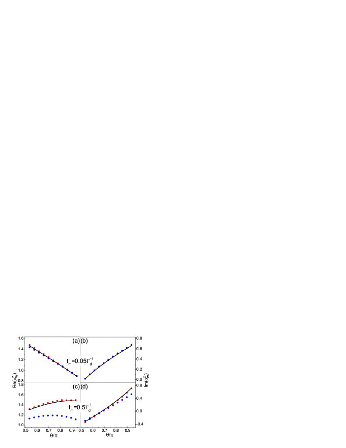
Figure 1: Extracted AAV WVs versus the post-selection state (characterized by its polar angle $\theta$). The correction effect of the second ${\cal G}$ term in the denominator of Eq. (14) is illustrated through its inclusion (red dots) and neglect (blue dots), in comparison with the “true” values (solid curves). Two strengths of measurement are considered: in (a) and (b), $t_{m}=0.05\Gamma^{-1}_{d}$; in (c) and (d), $t_{m}=0.5\Gamma^{-1}_{d}$. Parameters: $\Delta_{r}=0$, $\epsilon_{m}=1.0$, $\chi=0.1$, and $\kappa=8.0$.

In Fig. 1 we display the extracted AAV WV against the post-selection state $|\psi_{f}\rangle$. Our main interest here is the correction effect of the second ${\cal G}$ term in the denominator of Eq. (14). We thus simulate two strengths of measurement by choosing the measurement time $t_{m}=0.05\Gamma_{d}^{-1}$ for Fig. 1 (a) and (b), and $t_{m}=0.5\Gamma_{d}^{-1}$ for (c) and (d). We compare the AAV WVs (the red and blue dots) extracted from Eq. (14) with the “true” results (solid lines) calculated using Eq. (15) with the “testing” state $|\psi_{i}\rangle$. The results of the red dots are extracted from the full formula of Eq. (14), while the blue dots are from neglecting the second ${\cal G}$ term in the denominator. We see that for vanishing strength of measurement, as shown in Fig. 1(a) and (b), the effect of the ${\cal G}$ term is negligible. However, for finite strength of measurement (Fig. 1(c) and (d)), one must take into account the ${\cal G}$ term.

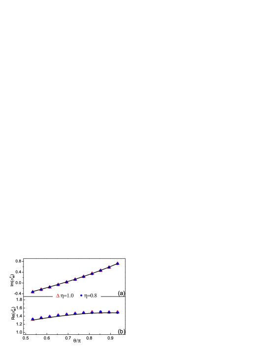
Figure 2: AAV WVs extracted from the PPS averages under ideal ($\eta=1$) and non-ideal ($\eta=0.8$) measurements, in comparison with the “true” values (solid curves). Parameters: $\Delta_{r}=0$, $\epsilon_{m}=1.0$, $\chi=0.1$, $\kappa=8.0$, and $t_{m}=0.5\Gamma^{-1}_{d}$.

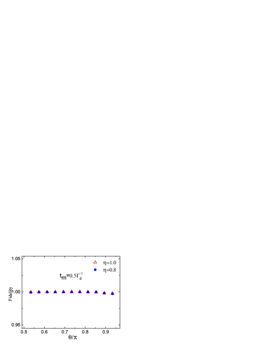
Figure 3: Alternative plot of the result in Fig. 2, via the fidelity of the estimated state $\rho$ with respect to the “true” one, $\varrho_{i}=|\psi_{i}\rangle\langle\psi_{i}|$, using $F={\rm Tr}(\varrho_{i}\rho)$.

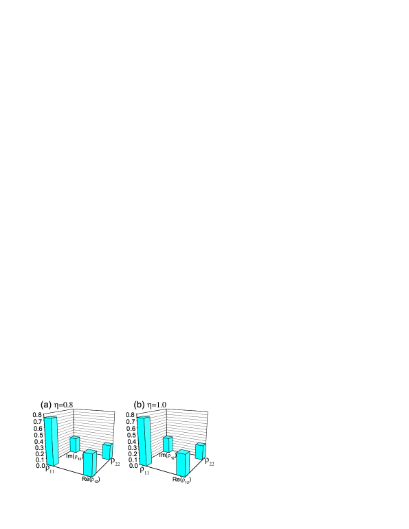
Figure 4: Tomographic plot of the estimated state from the result in Fig. 2 (an example using post-selection with $\theta=0.65\pi$). Detailed numerics: The “true” (unknown) state was set as $\varrho_{i,11}=0.75$ and $\varrho_{i,12}=0.34+0.265i$. The state estimated from ideal measurements ($\eta=1$) is $\rho_{11}=0.75095$ and $\rho_{12}=0.33218+0.27691i$, while the result from $\eta=0.8$ reads $\rho_{11}=0.74891$ and $\rho_{12}=0.3356+0.27461i$.

We now turn to an important issue related to the state tomography under present investigation. That is, this scheme is free from the efficiency of the quantum weak measurement. This unexpected feature is rooted in a finding in our previous study Li15 , where the weak values of qubit measurements were found free from the quantum efficiency of the measurements. Note that, in sharp contrast with this, state tracking by continuous weak measurement and quantum feedback control, would essentially depend on the efficiency of the quantum measurements. Non-ideal measurements will degrade the fidelity of the controlled target state, or completely lose all the state information. This drawback is actually the main obstacle of quantum feedback control in the circuit QED systems Sid12 .

Within the Bayesian formalism, we simply account for the measurement inefficiency by inserting a decoherence factor $e^{-(1-\eta)\Gamma_{m}t_{m}}$ into the off-diagonal elements of the qubit state. This treatment has qualitatively included the consequences of such as the amplifier’s noise in the homodyne measurement and the loss of measuring photons. Accordingly, in running the effective quantum trajectory equation Li15 ; Gam08 , we reduce, simultaneously, the rates $\Gamma_{ci}$ and $\Gamma_{ba}$ by a factor “$1-\eta$”.

In Fig. 2 we compare the AAV WV extracted from the ideal measurement (red triangles, with $\eta=1$) with the one under efficiency $\eta=0.8$ (blue dots), while plotting both against the “true” result (solid curve). Indeed, we find all the three results in perfect agreement. In Fig. 3 we further display the fidelity of the estimated state $\rho$ with respect to the “true” one, $\varrho_{i}=|\psi_{i}\rangle\langle\psi_{i}|$, using the fidelity definition $F={\rm Tr}(\varrho_{i}\rho)$, while in Fig. 4 we characterize, for a specific example, the full state (diagonal and off-diagonal elements of the density matrix) in terms of the usual means of quantum state tomography. Through these plots, we illustrate that, indeed, the direct (weak value associated) scheme of quantum state tomography is free from the efficiency of quantum measurement.

Now let us consider the situation beyond the bad-cavity and weak response limits, and illustrate how to reliably extract the AAV WV and determine the qubit state. We set $\kappa=2$ and remain all the other parameters the same as used in Figs. 1-4. In this case, if we improperly use Eq. (14) with all the rates and the ac-Stark shift determined by the steady-state cavity fields, as indicated by the blue dots in Fig. 5, the extracted AAV WV will suffer serious error from the “true” result. However, instead, if we combine Eq. (14) with the factors given by Eq. (II.4), satisfactory results can be obtained, as shown in Fig. 5 by the red dots. This ensures that the direct scheme of state tomography can be applied beyond the bad-cavity and weak response limits, if one properly applies Eqs. (14) and (II.4).

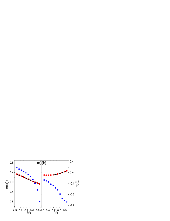
Figure 5: AAV WVs extracted from measurements beyond the bad-cavity and weak response limits. Red dots: results extracted correctly using Eq. (14) together with the factors Eq. (II.4). Blue dots: results extracted improperly using Eq. (14) under steady state of the cavity fields, as done in the bad-cavity and weak response limits. The “true” results are displayed by the solid curves. Parameters: $\Delta_{r}=0$, $\epsilon_{m}=1.0$, $\chi=0.1$, $\kappa=2.0$, and $t_{m}=0.5\Gamma^{-1}_{d}$.

IV Summary and Discussion

We have presented a new scheme for qubit state tomography

in the superconducting circuit-QED system, based on weak measurements and the associated quantum Bayesian approach. The Bayesian approach allows us to derive a compact expression for the PPS average, which encodes the full information of the AAV WV and makes the participation of its real and imaginary parts tunable by modulating the LO phase of the homodyne measurement. For the first time, we also obtained analytic expression for the PPS average beyond the bad-cavity and weak-response limits, and demonstrated how to determine the qubit state in this regime.

We may stress that, in order to reduce the measurement disturbance on the measured state, “weakness” of measurement is usually required to the weak-value-based direct scheme. However, differing from state tracking and feedback control, the direct state tomography is free from the efficiency of the quantum weak measurement. This feature is out of simple expectation, since the non-ideality of measurement will affect state inferring conditioned on the measurement results, and thus affect the success probability of post-selection. The key point is that the PPS average is free from the efficiency of measurement. This efficiency-free feature can greatly benefit the implementation of the proposed scheme in experiments.

It would be of interest to explore the direct scheme of state tomography for more complicated states, e.g., entangled state of multiple qubits, and nontrivial quantum state of cavity fields. We may leave such sort of problems for future investigations.

Acknowledgments.

— This work was supported by the NNSF of China under grants No. 91321106 & 210100152, the State “973” Project under grant No. 2012CB932704, the Beijing NSF under grant No. 1164014, and the Fundamental Research Funds for the Central Universities.

References

- (1) W. K. Wootters and W. H. Zurek, Nature 299, 802 (1982).
- (2) K. Vogel and H. Risken, Phys. Rev. A 40, 2847 (1989).
- (3) D. T. Smithey, M. Beck, M. G. Raymer, and A. Faridani, Phys. Rev. Lett. 70, 1244 (1993).
- (4) G. Breitenbach, S. Schiller, and J. Mlynek, Nature 387, 471 (1997).
- (5) A. G. White, D. F. V. James, P. H. Eberhard, and P. G. Kwiat, Phys. Rev. Lett. 83, 3103 (1999).
- (6) M. Hofheinz et al., Nature 459, 546 (2009).
- (7) J. S. Lundeen, B. Sutherland, A. Patel, C. Stewart, and C. Bamber, Nature 474, 188 (2011).
- (8) J. S. Lundeen and C. Bamber, Phys. Rev. Lett. 108, 70402 (2012).
- (9) J. Z. Salvail, M. Agnew, A. S. Johnson, E. Bolduc, J. Leach, and R. W. Boyd, Nature Photonics 7, 316 (2013).
- (10) M. Malik, M. Mirhosseini, M. P. J. Lavery, J. Leach, M. J. Padgett, and R. W. Boyd, Nature Communications 5, 3115 (2014).
- (11) Y. Aharonov, D. Albert, and L. Vaidman, Phys. Rev. Lett. 60, 1351 (1988).
- (12) I. M. Duck, P. M. Stevenson, and E. C. G. Sudarshan, Phys. Rev. D 40, 2112 (1989).
- (13) Y. Aharonov and L. Vaidman, Phys. Rev. A 41, 11 (1990).
- (14) N. W. M. Ritchie, J. G. Story, and R. G. Hulet, Phys. Rev. Lett. 66, 1107 (1991).
- (15) H. Wiseman, Phys. Rev. A 65, 032111 (2002).
- (16) D. R. Solli, C. F. McCormick, R. Y. Chiao, S. Popescu, and J. M. Hickmann, Phys. Rev. Lett. 92, 043601 (2004).
- (17) L. Johansen, Phys. Rev. Lett. 93, 120402 (2004).
- (18) G. J. Pryde, J. L. O’Brien, A. G. White, T. C. Ralph, and H. M. Wiseman, Phys. Rev. Lett. 94, 220405 (2005).
- (19) O. Hosten, and P. Kwiat, Science 319, 787 (2008).
- (20) P. B. Dixon, D. J. Starling, A. N. Jordan, and J. C. Howell, Phys. Rev. Lett. 102, 173601 (2009).
- (21) S. Kocsis et al., Science 332, 1170 (2011).
- (22) A. Feizpour, X. Xing, and A. M. Steinberg, Phys. Rev. Lett. 107, 133603 (2011).
- (23) A. Blais, R. S. Huang, A. Wallraff, S. M. Girvin, and R. J. Schoelkopf, Phys. Rev. A 69, 062320 (2004).
- (24) A. Wallraff, D. I. Schuster, A. Blais, L. Frunzio, R. S. Huang, J. Majer, S. Kumar, S. M. Girvin, and R. J. Schoelkopf, Nature 431, 162 (2004).
- (25) R. Vijay, C. Macklin, D. H. Slichter, S. J. Weber, K. W. Murch, R. Naik, A. N. Korotkov and I. Siddiqi, Nature 490, 77 (2012).
- (26) M. Hatridge, S. Shankar, M. Mirrahimi, F. Schackert, K. Geerlings, T. Brecht, K. M. Sliwa, B. Abdo, L. Frunzio, S. M. Girvin, R. J. Schoelkopf, and M. H. Devoret, Science 339, 178 (2013).
- (27) K. W. Murch, S. J. Weber, C. Macklin and I. Siddiqi, Nature 502, 211 (2013).
- (28) D. Tan, S. J. Weber, I. Siddiqi, K. Molmer, and K.W. Murch, Phys. Rev. Lett. 114, 090403 (2015).
- (29) N. S. Williams and A. N. Jordan, Phys. Rev. Lett. 100, 026804 (2008).
- (30) L. Qin, P. Liang, and X. Q. Li, Phys. Rev. A 92, 012119 (2015).
- (31) J. Gambetta, A. Blais, M. Boissonneault, A. A. Houck, D. I. Schuster, and S. M. Girvin, Phys. Rev. A 77, 012112 (2008).
- (32) A. N. Korotkov, Phys. Rev. B 60, 5737 (1999).
- (33) A. N. Korotkov, Quantum Bayesian approach to circuit QED measurement, arXiv:1111.4016
- (34) P. Wang, L. Qin, and X. Q. Li, New J. Phys. 16, 123047 (2014); ibid. 17, 059501 (2015).
- (35) W. Feng, P. Liang, L. Qin, and X. Q. Li, Sci. Rep. 6, 20492 (2016).